Constrained Multi-user Multi-server Max-Min Fair ... - Semantic Scholar

1

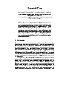
Constrained Multi-user Multi-server Max-Min Fair Queuing∗

arXiv:1601.04749v1 [cs.NI] 18 Jan 2016

Jalal Khamse-Ashari, Ioannis Lambadaris, Yiqiang Zhao

Abstract—In this paper, a multi-user multi-server queuing system is studied in which each user is constrained to get service from a subset of servers. In the studied system, rate allocation in the sense of max-min fairness results in multi-level fair rates. To achieve such fair rates, we propose CM 4 F Q algorithm. In this algorithm users are chosen for service on a packet by packet basis. The priority of each user i to be chosen at time t is determined based on a parameter known as service tag (representing the amount of work counted for user i till time t). Hence, a free server will choose to serve an eligible user with the minimum service tag. Based on such simple selection criterion, CM 4 F Q aims at guaranteed fair throughput for each demanding user without explicit knowledge of each server service rate. We argue that CM 4 F Q can be applied in a variety of practical queuing systems specially in mobile cloud computing architecture. Index Terms—Fair Queuing, multi-level Max-Min Fairness, Packet scheduling, Mobile Cloud Computing

I. I NTRODUCTION

M

AX-MIN Fairness has been known as the most prevalent notion of fairness in the concept of resourceallocation. In allocating one type of resource to some demanding users, an allocation is said to be max-min fair, if it is feasible and an increase in the amount of allocated resource to any arbitrary user, results in decreasing the amount of allocated resource to some other user(s) with smaller or equal allocation [1]. If the resource can be divided into any arbitrary parts and each user is eligible to use any part of the resource, maxmin fair allocation results in equal shares for different users. When the resource comprises of only one indivisible part (one server), time sharing or “scheduling” is the natural way for multiplexing. Considering a set of greedy users, max-min fairness could be defined in this case based on the users’ longterm/average usage of the resource [1]. When the resource is arbitrarily divisible, max-min fair allocation could be defined in terms of instantaneous usage. Specifically, consider resources such as bandwidth or CPU. When such resources are arbitrarily divisible, max-min fair allocation could be defined in terms of instantaneous rates. This approach has been known as Weighted Fair Sharing (WFS). By definition, in weighted fair sharing equal weighted rates are attributed to demanding users at any time t [2]. The most important property of WFS is being memoryless, i.e., each user’s current rate of service is independent of its * Work in progress, version 1. Khamse-Ashari and Lambadaris are with the SCE department, Zhao is with the School of Mathematics and Statistics, Carleton University, Ottawa, Canada.

𝑓𝑙𝑜𝑤 𝑎

𝑓𝑙𝑜𝑤 𝑏

2.5 𝑀𝑏𝑝𝑠 1 𝑀𝑏𝑝𝑠

𝑓𝑙𝑜𝑤 𝑐

𝜑𝑎 = 𝜑𝑏 = 𝜑𝑐 = 1 Fig. 1. A sample queuing system; Users a and b are eligible to get service from both servers, while user c is only eligible to get service from server 2.

rate of service in the past. This is specially important when users have intermittent demands. According to memoryless property, if user i has not any demand of the resource during interval (t0 , t1 ), its share of service is not reserved [2], [3]. Instead, it could be divided among other demanding users. The memoryless property is central in guaranteeing that users will not be starved in a work-conserving system. When the resource comprises of only one indivisible part (i.e., one server), WFS could be realized if users’ demands are infinitesimally divisible, i.e. represented by fluid flow [2], [3]. When users’ demand or “input traffic” is packetized, WFS could be achieved only approximately through packet by packet scheduling schemes [4]. Many Fair Queuing (FQ) algorithms have been proposed to approximate WFS on a packet by packet scheduling basis. Self-Clocked Fair Queuing (SCFQ) is the first practically implementable algorithm achieving a good approximation of WFS [4]. In this paper, a system model is considered in which one type of resource, like CPU or bandwidth, is available on multiple servers. In addition, it is assumed that each user is eligible to get service only from a subset of servers. Considering such a constrained multi-user multi-server queuing system, max-min fair rate allocation results in multi-level fair rates. As an example, consider the queuing system shown in Fig.1. Assume traffic stream of users to be fluid flow. According to max-min fairness definition (mentioned in the beginning of the introduction), the max-min fair rate of user c equals to rc (t) = 1 Mbps, while the max-min fair rate of users a and b equal to ra (t) = rb (t) = 1.25 Mbps. In such allocation, the service rate of server 1 is equally divided between users a and b, while the total service rate of server 2 is allocated to user c. While there exists a rich literature on FQ, e.g., [3], [4], [5], [6], [7], [8], none of algorithms developed in the context of FQ is applicable for the case of constrained multi-user multi-

2

𝑓𝑙𝑜𝑤 1

𝜑2

𝑓𝑙𝑜𝑤 2

𝑆1 𝑆2

𝜑𝑁 𝑓𝑙𝑜𝑤 𝑁

…

1 CM 4 F Q stands for Constrained Multi-user Multi-server Max-Min Fair Queuing.

𝜑1

…

server queuing system. Indeed, all existing FQ algorithms are designed to achieve equal fair rates among demanding users. For instance, while [6] has considered a multi-server queuing system, it has considered the case that any user is eligible to get service from any server. As a consequent, in such fully connected system all users attain the same fair service rate. Hence, the proposed FQ algorithm in [6] is essentially the same as a single server FQ algorithms. Regarding multi-level max-min FQ, the literature is very sparse. To the best of our knowledge, there is not any prior work which addresses multi-level max-min FQ problem in general. We have seen prior work in [9] which has studied the same constrained multi-user multi-server queuing system. After presenting our proposed FQ algorithm and showing its generality, we will compare it with the results of [9] in Section VII. Considering the constrained multi-user multi-server queuing model, in this paper we propose a FQ algorithm which we call CM 4 F Q1 . This algorithm is designed to achieve multi-level max-min fair rates. Like in single server FQ algorithms, in CM 4 F Q packets scheduling decisions are made simply based on the users’ service tag. Service tag of each user i represents the amount of work counted for user i till time t. Given that server k becomes free at time t, it will choose to serve the user with the minimum service tag among users eligible to get service on this server. Based on such simple selection criterion, CM 4 F Q aims at guaranteed fair throughput for each demanding user without explicit knowledge of each server service rate. While CM 4 F Q addresses a general system model, it is very simple. Hence, it can be applicable in different scenarios. For example, in mobile cloud computing networks [10], multiple servers/machines are available for giving service to different applications/queues. Each server possibly has different amounts of resources, including CPU, RAM, etc. In correspondence with our queuing model, CPU could be considered as the scarce resource which is to be scheduled among users. On the other hand, each application possibly has different requirements of RAM, storage, etc., which may be available only on a subset of servers. These requirements could be reflected as certain constraints for each application to get service from different servers. Another application conforming to the described system model, is related to smart mobile phones which have several interfaces for data access [9]. Specifically, mobile phones may have data access via WiFi, 3G or 4G at the same time. On the other hand, there are certain restrictions for mobile applications to use different access techniques. For example, it may be preferred to stream video only over WiFi because it is cheaper, but to use the more expensive available data rate of 3G for VoIP. Reflecting such preferences as constraints on choosing different interfaces by each application, our proposed algorithm could be used for fair packet scheduling. The rest of this paper is organized as follows. Basic definitions and system model are stated in section II. Our proposed

𝑆𝐾

Fig. 2. System model (any user eligible to get service from a server is connected to that by an arrow)

FQ algorithm is described in section III. Section IV and V are devoted to characterizing properties and performance of the proposed FQ algorithm. Our analytical results are evaluated through numerical studies in section VI. After a brief review of related works in section VII, our conclusions are drawn in section VIII. II. BASIC D EFINITIONS AND S YSTEM M ODEL A. System Model Consider a multi-user multi-server queuing system as shown in Fig. 2 in which each user is constrained to get service from a subset of servers. Assume that N = {1, 2, ..., N } is the set of users and K= {1, 2, ..., K} is the set of servers. The service rate function of each server k is ρk (t) bits/sec. Let a binary matrix denoted by Π = [πi,k ], determines the constraints of users to get service from different servers. Therefor, user i is eligible to use server k when πi,k = 1, and is not eligible otherwise. There exists at least a single “1” element in each row and each column of the matrix Π, i.e., any user (server) is connected to at least one server (user). To present the notion of max-min fairness in this scenario, first consider users’ input traffic streams as fluid flow. Assuming an idealized fluid flow system, some basic definitions are presented in the next subsection. B. Basic Definitions Definition 1: Any arbitrary user i is said to be backlogged at time t, if its corresponding queue is not empty at time t− . The set of backlogged users at time t is denoted by B(t). Definition 2: In an idealized fluid flow system conforming to the system model of Fig. 2, let ri,k (t) be the service rate allocated to user i by server k. The matrix R(t) = [ri,k (t)]N ×K satisfying the following conditions is defined as a rate allocation matrix. a) If user i is not backlogged at time t, then ri,k (t) = 0, ∀k ∈ K. b) For any user i ∈ N and server k ∈ K, if πi,k = 0 then ri,k (t) = 0. c) If at least one of users eligible toPget service from server k is backlogged at time t, then i∈N ri,k (t) = ρk (t). The above conditions guarantee the queuing system to be work conserving. According to the rate allocation matrix R(t) = [ri,k (t)], the total service rate Pallocated to an arbitrary user i at time t is equal to ri (t) = k∈K ri,k (t).

3

Suppose that a positive wight ϕi > 1 is associated to each user i. Using the weight associated to user i, the normalized service rate of user i is defined as ri (t)/ϕi . Definition 3: A rate allocation mechanism is said to be memoryless if the service rate of each user at time t is independent of its service rate for all times prior to t, [3]. Definition 4: (CM 4 fairness) A rate allocation matrix R(t) is said to satisfy Constrained Multi-user Multi-server Max-Min (CM 4 ) fairness, when increasing the normalized service rate of any user results in decreasing the normalized service rate of some other user(s) with smaller or equal normalized service rate. It should be mentioned that CM 4 fairness is just the general definition of max-min fairness which has been applied to the rate allocation in the constrained multi-user multiserver queuing system [1], [9]. Since CM 4 fair rate allocation is defined in terms of instantaneous rates, it is obviously memoryless. Theorem 1: Consider a fluid flow system conforming to the system model of Fig. 2. A rate allocation matrix R(t) satisfies CM 4 fairness, if and only if statement (1) holds for any backlogged user j: if ri,k (t) > 0 and πj,k = 1 ⇒

ri (t) rj (t) ≥ φj φi

(1)

Theorem 1, that is a concise statement of Theorem 2 in [9], offers a necessary and sufficient condition on R(t) to be fair in conjunction with CM 4 fairness definition. Since the proof follows the same line of arguments as what provided for Theorem 2 in [9], it is omitted here. To get a better intuition on the concept of CM 4 fairness, we consider an example. Example 2.1: Consider the queuing system shown in Fig. 3. Assume traffic stream of users to be fluid flow. According to CM 4 fairness definition, the fair service rate of user d equals to 1 Mbps, while the fair service rate of users a, b and c equals to 1.2 Mbps. To achieve such fair service rates, the total service rate of server 3 should be allocated to user d. However, there exist several ways for allocating the service rate of server 1 and server 2 to users a, b and c, while each of them gets a service rate of 1.2 Mbps. The reader can verify that in this example there are more than one rate allocation matrices satisfying CM 4 fairness. However, all of such matrices share some common properties. First, in all cases users a, b and c get the same service rate. Second, in all of them users with higher service rate are not given service on the server allocated to the user with lower service rate. Based on these observations, the set of users and servers could be classified into two clusters (Fig. 3), satisfying the following conditions. I) Users in each cluster have the same fair service rates. II) All users in a cluster are only given service by servers in that cluster. In the following, the concept of clustering is defined in general for any arbitrary configuration of users and servers. A cluster C(t) is defined as an ordered pair C(t) = (I(t), S(t)), where I(t) and S(t) are non-empty subset of users and non-empty subset of servers, respectively. Suppose that all users are partitioned into M disjoint subsets Im (t), 1 ≤ m ≤ M and all servers are partitioned into the

𝑓𝑙𝑜𝑤 𝑎

𝑓𝑙𝑜𝑤 𝑏

𝑆1 1.8 𝑀𝑏𝑝𝑠

𝑓𝑙𝑜𝑤 𝑐

𝑆2 1.8 𝑀𝑏𝑝𝑠

𝑓𝑙𝑜𝑤 𝑑

𝑆3

1 𝑀𝑏𝑝𝑠

Fig. 3. A sample queuing system, the weight of all users are assumed to be equal. Here there are two clusters, C1 = ({a, b, c}, {s1 , s2 }), C2 = ({d}, {s3 }). The normalized service rate of users in cluster 1 is rC1 = 1.2 Mbps, and the normalized service rate of user d in cluster 2 is rC2 = 1 Mbps.

same number M disjoint subsets Sm (t), 1 ≤ m ≤ M . A clustering consisting of M clusters is defined as {Cm (t)}M m=1 , where Cm (t) = (Im (t), Sm (t)). Definition 5: Suppose the rate allocation matrix R(t) satisfies CM 4 fairness when B(t) = B is the set of backlogged users at time t. Clustering {Cm (t)}M m=1 is said to be a Fairness Oriented Clustering (FOC) in conjunction with B if: a) For any cluster Cm (t), any user i ∈ Im (t) has the same normalized service rate, ri (t)/ϕi = rCm (t). We define rCm (t) as the cluster service rate. b) For any two distinct clusters Cm (t) and Cl (t), m 6= l, rCm (t) 6= rCl (t). c) Server k belongs to cluster Cm (t) with rCm (t) > 0, if and only if ri,k (t) > 0 for some user i ∈ Im (t). Lemma 1: For given set of backlogged users and service rates of servers, there exists a unique FOC. For a given set of backlogged users at time t, B(t) = B, it may be possible that more than one rate allocation matrices satisfying CM 4 fairness exist. However, Lemma 1 implies that all of them result in the same unique FOC. The proof of Lemma 1 can be found in the appendix. A similar clustering method referred to as rate clustering is presented in [9]. Indeed, the FOC satisfies the rate clustering property. However, the rate clustering does not result in a unique clustering for a given set of backlogged users. Fact 1: For given service rate of servers, FOC at time t0 could be viewed as a function of the set of backlogged users B0 = B(t0 ), i.e., {Cm (B0 )}M m=1 . It is straightforward to show that for any two clusters m, l such that rCm > rCl , any user i in Cl can not be eligible for getting service from servers k in cluster Cm (i.e., πi,k = 0). This is formally stated in the following corollary. Corollary 1: Let {Cm (t)}M m=1 be the FOC which corresponds to the set of backlogged users B = B(t). If some user j ∈ Im (t) with positive service rate is eligible to get service from server k in another cluster, πj,k = 1 and k ∈ Sl (t), then it follows that rCm (t) > rCl (t).

4

III. FQ A LGORITHM 4

An FQ algorithm that achieves CM fairness is proposed in this section. Although in the introductory material presented thus far we mainly focused on (idealized) fluid flow system, the algorithm that we will develop operates on packet by packet basis. In particular, when a server becomes free, the algorithm decides on which packet to be served by that server, while respecting users service constraints (determined by matrix Π). Any packet chosen to get service from a server, gets all of its service from that server without any interruption. Since the algorithm works on a packet-by-packet basis, each user could achieve its fair service rate in an “approximate” fashion. More specifically, consider an interval (t1 , t2 ) during which the set of backlogged users does not change. According to CM 4 fairness definition, for the same set of backlogged users in an idealized fluid flow system, each backlogged user has a specific fair service rate, and therefor each backlogged user has a specific fair service (work) share for that interval. In Section V, it is shown that the difference between the amount of work offered in [t1 , t2 ) to any backlogged user by CM 4 F Q algorithm in the actual system vs its fair share within [t1 , t2 ) in an idealized fluid flow system with the same set of backlogged users remains bounded. Before presenting the algorithm, we introduce some notation along with assumptions. A. Notation and Assumptions •

• •

•

It is assumed that each server can hold only one packet under service. When user i is chosen for service by server k, its head of queue packet is moved to the server. The server keeps the packet till its service is completed. It is assumed that service rate of each server k is time invariant2 , i.e., ρk (t) = ρk for all t. According to Definition 1, a user is said to be backlogged at time t, if its corresponding queue is not empty at time t− . Hence, a user with empty queue and some packets under service is not considered to be backlogged. The set of backlogged users at time t which are eligible to get service from server k is denoted by B k (t): B k (t) , {i | i ∈ B(t) and πi,k = 1}.

• • •

(2)

Server k is said to be backlogged at time t, if B k (t) 6= ∅. All functions of time in this paper are assumed to be left continuous, i.e.,: f (t− ) = f (t). For any scalar function f (t), f (t1 , t2 ) is defined as f (t1 , t2 ) = f (t2 ) − f (t1 ). It is assumed that packets of each user have a maximum length of Lmax bits. The length of each packet in bits is considered as the required work of that packet.

B. The CM 4 F Q Algorithm CM 4 F Q algorithm belongs to the class of FQ algorithms. In such algorithms, the priority of each user i to be chosen 2 Since the proposed algorithm works without explicit knowledge of each server service rate, it could be used even when servers have time varying service rates. However, for the sake of simplifying the presentation we make such assumption.

at time t is determined based on a parameter, Fi (t), which is computed through the algorithm and will be referred as service tag. CM 4 F Q assigns an individual service tag to each user3 ; Fi (t) represents the amount of work counted for user i through the execution of the algorithm till time t. Fi (0) is initially set as zero for all users. At time t a free server will choose to serve an eligible user with the minimum service tag. For any server k a function V k (t) is defined to represent the work level of server k at time t. For server k with nonempty set of backlogged users (B k (t) 6= ∅), V k (t) will be set to the minimum service tag of users i ∈ B k (t). For the case where the set B k (t) is empty, V k (t) will be set to ∞. Therefor, V k (t) is defined by: k

V (t) ,



min{Fj (t) | j ∈ B k (t)} ∞

if B k (t) 6= ∅ otherwise

(3)

Intuitively, V k (t) gives a measure of work progress in the system till time t from the perspective of server k. Work level of servers at time t, will be used in updating the service tag of an idle user which becomes backlogged at time t. We will now present the algorithm which is summarized in table I. In order to get intuition and understand its de-queuing mechanism, we assume that server k becomes free at time t. Among backlogged users eligible to get service from this server, the head of queue packet of user i∗ with the minimum of Fi (t) is chosen for service (as stated in (5)). In case of a tie, the user with the minimum index is chosen. Given that packet p of user i∗ is chosen for service, Fi∗ (t+ ) is incremented by Lp /ϕi∗ (as stated in (6)), where Lp is the length of packet p in bits, and ϕi∗ as stated previously represents the weight for user i∗ 4 . If user i∗ is chosen for service by server k, its head of queue packet is removed and goes to the server. This is the task of Dequeue(·) function shown in table I. It also checks the queue of user i∗ to determine whether it is backlogged. If user i∗ is not backlogged anymore, it updates the set of backlogged users. Upon selection of packet p of user i∗ for service, its service tag is incremented by Lp /ϕi∗ . Taking this into account, the work level of servers eligible to give service to user i∗ should be updated (This is performed by (9) and (10) in U pdateV (i∗ , k) subroutine). Therefor, at any time during the execution of the algorithm, V k represents work progress from server’s k perspective. To understand the en-queuing mechanism (En-queuing module in the algorithm of Table I), assume that user i becomes backlogged after a period of idleness. In order to achieve the memoryless behaviour, user i should not claim its share of service of the idle period from none of the servers. Therefor, Fi is updated to max{Fi , max{V k | πi,k = 1}}, which is 3 In correspondence with FQ algorithms like SFQ or SCFQ [4], [5], F (t) i represents “Finish Service Tag” of the last packet of user i which has been chosen to get service before time t From another perspective, for user i being backlogged at time t, Fi (t) represents “Start Service Tag” of its head of queue packet. 4 For the sake of simplicity, the time index for all parameters will be omitted in the pseudo-code representation of the algorithm.

5

TABLE II T HE SUBROUTINES OF CM 4 F Q A LGORITHM

TABLE I T HE PSEUDO CODE OF CM 4 F Q A LGORITHM CM 4 F Q Algorithm • •

Initialization

ActivateServers(i) V 0 = 0; If ({k | V k < ∞} 6= ∅)

For (i = 1; i ≤ N ; i + +) Fi = Di = 0; For (k = 1; k ≤ K; k + +)

V 0 = max{V k | V k < ∞} + δ;

V k = Dk = 0; •

V l = V 0;

En-queuing Module: On arrival of packet p of user i

•

If (Empty(Queuei )) Fi = max{Fi , max{V k | πi,k = 1}}; (4) Enqueue(i, p); //Enqueue packet p to queue of user i and update B

UpdateV(i, k)

For (l = 1; l ≤ K & πi,l = 1; l + +) V l = ∞;

(9)

If (B l 6= ∅) V l = min{Fj | j ∈ B l } (10) //regulating the gap among work level of servers

De-queuing Module(server k) While(B k 6= ∅) i∗ ← argmini {Fi | i ∈ B k };

(8)

//updating work level of servers Vˆ k = V k ;

Activate-Servers(i)

•

(7)

For (l = 1; l ≤ K & πi,l = 1 & V l = ∞; l + +)

(5)

p = Dequeue(Head(Queuei∗ )); //Dequeue head of queue of user i and update B Lp = Size(p); Fi∗ = Fi∗ + Lp /ϕi∗ ; (6) U pdateV (i∗ , k); Service(k, p); //Give service to packet p on server k

dk = 0; If ({l | V l < Vˆ k } 6= ∅) dk = min{V l | Vˆ k ≤ V l } − max{V l | V l < Vˆ k } − δ;

(11)

If (dk > 0) For (j = 1; j ≤ N & Fj ≥ Vˆ k ; j + +) Fj = Fj − dk ;

(12)

Dj = Dj + dk ;

(13)

For (l = 1; l ≤ K & V l ≥ Vˆ k ; l + +) k

greater than or equal to V , for any server k that is eligible to give service to user i, ((4) in Table I). To provide a better understanding of the algorithm, we consider some illustrative examples. In these examples, we assume that U pdateV (i∗ , k) subroutine is restricted to updates in (9) and (10) and other updates in it are not implemented. The resultant algorithm will be referred to as reduced CM 4 F Q algorithm. The first example describes the role of ActivateServers(·) subroutine. The second example examines the role of (4) by which Fi is updated for a returning customer i. The third example, reveals the shortage of the reduced CM 4 f Q algorithms to achieve fairness and shows the necessity for additional updates (i.e. (11)-(15)) in U pdateV (i, k) subroutine of Table II. Example 3.1: Consider again the queuing system shown in Fig. 1. Assume that input traffic stream of users comprises of packets of fixed length L = 1000 bits. User c is assumed to be continuously backlogged since t = 0. It is assumed that 13 packets already exist in the queue of each user a and b at time t = 0. It is assumed that no packet arrives at these queues during [0, t1 ), till t1 = 20 msec. Users a and b are assumed to become backlogged at t+ 1 and remains backlogged afterwards. Applying the reduced CM 4 F Q algorithm, it can be observed that all existing packets in the queue of users a and b at t = 0 are given service during interval [0, t0 ), where t0 = 10 msec. In fact, the last existing packet in the queue of user b is chosen by server 1 at 9.6 msec. Hence, Fa and Fb remain constant during (9.6, 20) msec. On the other hand, Fc

V l = V l − dk ;

(14)

D l = D l + dk ;

(15)

increases with an average rate of 1 Mbps. Hence, Fc is greater than Fa and Fb at time t1 (as shown in Fig. 4). At time 9.6 msec that the set of backlogged users connected to server 1, B 1 becomes empty, V 1 is set to ∞ (as stated in 9). The role of ActivateServers(·) subroutine is to reset the work level of this server to a proper finite value as soon as it becomes backlogged. Given that user a and user b become 1 2 backlogged at t+ 1 , V will be updated to V + δ ((8) and (8) in ActivateServers(·) subroutine), where δ is assumed to be δ = 2L. It can be observed that by updating V 1 in this way and by choosing δ = 2L, no packet of user a or user b is serviced on server 2 from time t1 onwards (Fig. 4). In contrast, if such an update were not performed or if δ were chosen equal to Lmax (or some smaller amount), it would be possible for users a and b to have some packets serviced on server 2. Example 3.2: Consider again the queuing system shown in Fig. 1. For simplicity assume Lmax , the maximum length of packets, to be infinitesimal (i.e., we consider fluid flow arrivals). Let users b and c be continuously backlogged since time t = 0. User a becomes backlogged at t0 = 100 msec, and remains backlogged afterwards. Applying the reduced CM 4 F Q algorithm, during interval (0, t0 ) user b gets a service rate of 2.5 Mbps from server 1 and user c gets a service rate of 1 Mbps from server 2. Work level of servers are shown

6

𝑓𝑙𝑜𝑤 𝑑

35 Fc= V2 30

Fb

2L

20

25 Amount of Work(Kbits)

22

18

20

𝑆1 2.5 𝑀𝑏𝑝𝑠

𝑓𝑙𝑜𝑤 𝑏

𝑆2 1 𝑀𝑏𝑝𝑠

22

20

15

𝑓𝑙𝑜𝑤 𝑐

𝑓𝑙𝑜𝑤 𝑎

10

1 𝑀𝑏𝑝𝑠

5

𝑓𝑙𝑜𝑤 𝑐

𝜑𝑎 = 𝜑𝑏 = 𝜑𝑐 = 1

0

t1

t0 0

5

10

15

20

time 30 (ms)

25

Fig. 4. Service tag of users b and c, Fb (t) and Fc (t) in the network of Fig. 1. Except the interval (9.6, 20] msec, users a and b are backlogged elsewhere. Users c, is continuously backlogged since t = 0 (Example 3.1). 400 Fa 350

slope: 1.25 Mbps

V1 V2

300

250

200

slpoe: 1 Mbps slope: 2.5 Mbps

150 𝑓𝑙𝑜𝑤 𝑎

100

2.5 𝑀𝑏𝑝𝑠

𝑓𝑙𝑜𝑤 𝑏

50

1 𝑀𝑏𝑝𝑠 𝑓𝑙𝑜𝑤 𝑐

0

𝜑𝑎 = 𝜑𝑏 = 𝜑𝑐 = 1

t0 0

20

40

60

80

100

120

𝜑𝑎 = 𝜑𝑏 = 𝜑𝑐 = 𝜑𝑑 = 1

2.5 𝑀𝑏𝑝𝑠

𝑓𝑙𝑜𝑤 𝑏

Amount of Work (K bits)

𝑓𝑙𝑜𝑤 𝑎

18

140

160

180

time 200 (ms)

Fig. 5. Work level of servers, V k (t) (k = 1, 2) and service tag of user a, Fa (t) in the network of Fig. 1 (Example 3.2).

in Fig. 5 as function of time. When user a becomes backlogged at t0 , Fa (t+ 0 ) will be updated from 0 to max{V k (t0 ) | πa,k = 1}, (as stated in (4) and shown in Fig. 5). This way of updating has some consequences. First, Fa (t+ 0 ) becomes greater than or equal to V k (t0 ), for any server k that is eligible to give service to user a. Hence, user a does not claim its share of service of the idle period from non of the servers (memoryless property). Secondly, user a joins to the cluster with the maximum service rate available to it, i.e., it only gets service from servers 1. Sharing the total service rate of servers 1 between users a, b, each of them gets a service rate of 1.25 Mbps. On the other hand, user c gets 1 Mbps from server 2. It could be observed that by applying the reduced CM 4 F Q algorithm in this case, CM 4 fair service rates have been provided for all users. In this example, when user a becomes backlogged, it joins to the cluster with the maximum service rate available to it. As a result, the service rate of this cluster is reduced from 2.5 to 1.25 Mbps (Fig. 5). However, the configuration of clusters (in terms of servers) is not changed. In general, when some users change their states from backlogged to non-backlogged (or vice versa), the configuration of clusters could be changed entirely. The next example considers such a case.

Fig. 6. The queuing system of Example 3.3. Users a, b and c are continuously backlogged since t = 0. User d becomes backlogged at time t0 = 100msec, and remains backlogged afterwards.

Example 3.3: Consider the queuing system shown in Fig. 6. Let users a, b and c be continuously backlogged since t = 0. User d is assumed to become backlogged at t0 and remains backlogged afterwards. For the sake of illustration, suppose that the maximum length of packets is infinitesimally small (Lmax → 0). During interval (0, t0 ) that user d is not backlogged, the corresponding FOC consists of three clusters: C1 = ({a, b}, {S1 }), C2 = ({c}, {S2 }) and C3 = ({d}, {}), where rC1 = 1.25 Mbps, rC2 = 1 Mbps and rC3 = 0. After t0 that user d becomes backlogged, the corresponding FOC consists of only one cluster which contains all users and all servers, C = ({a, b, c, d}, {S1 , S2 }), where rC = 0.875 Mbps. Hence, the fact that user d becomes backlogged results in an entirely new FOC. Furthermore, by applying the reduced CM 4 F Q algorithm, it can be observed that during interval (0, t0 ) each user achieves its fair service rate. Specifically, Fa and Fb increase with a rate of 1.25 Mbps, while user c gets a service rate of 1 Mbps. Consequently, the rate of increase in V 1 is 1.25 times the rate of increase in V 2 (Fig. 7). Hence, as time passes by, a significant difference may form between V 1 and V 2 . Such a gap may potentially disturb fair performance of the reduced CM 4 F Q algorithm when the set of backlogged users changes. When user d becomes backlogged at time t0 = 100 msec, the fair service rate of each user will be 0.875 Mbps, i.e., the total capacity should be equally divided among the four users. Nevertheless, as long as V 1 is greater than V 2 (Fa and Fb are greater than Fc ), users a or b are not chosen by server 2 according to selection criterion in (5). Hence, users a and b get service only from server 1 during (t0 , t1 ), till t1 = 250 msec. In this interval, users a, b and d share server 1 getting 0.833 Mbps each, while user c gets a service rate of 1 Mbps. From time t1 when V 1 (t1 ) = V 2 (t1 ) (i.e., V 1 (t) and V 2 (t) cross), each user will get its fair rate of 0.875 Mbps, (Fig. 7). Example 3.3 shows that when the set of backlogged users changes, the gaps among work level of servers (as computed by the reduced CM 4 F Q algorithm) could disturb fair performance of the reduced CM 4 F Q algorithm during a considerable amount of time. In order to avoid this situation, for any server k the difference of V k and max{V l | V l < V k } is limited in CM 4 F Q algorithm to the predetermined parameter δ. Specifically, when this difference is exceeding δ (or equivalently dk that is defined in (11) becomes positive), the

7

300 V1 Fd

250

slope: 0.875 Mbps

Amount of work (K bits)

V2

𝑓𝑙𝑜𝑤 𝑎

𝑆1

𝜑𝑏 = 1

𝑓𝑙𝑜𝑤 𝑏

𝑆2 10 𝑀𝑏𝑝𝑠

1 𝑀𝑏𝑝𝑠

slope: 0.833 Mbps 200

Fig. 9. The queuing system of Example 3.5. Users are assumed to be continuously backlogged since t = 0.

slope: 1 Mbps

150 gap 100

slope: 1.25 Mbps

50

0

t0 0

50

100

150

200

t1

time

250

300 (ms)

Fig. 7. Work level of servers, V 1 (t) and V 2 (t), and service tag of user d, Fd (t) in the network of Fig. 6, when applying the reduced CM 4 F Q algorithm (Example 3.3). 55 50

V1

45

V2 Fb+Db

40 Amount of Work (Kbits)

𝜑𝑎 = 1

Average increasing rate: 1.25 Mbps

35 30 25 20

Average increasing rate: 1 Mbps

15 10 5

time 0

0

5

10

15

20

25

30

35

40 (ms)

Fig. 8. Work level of servers, V 1 (t) and V 2 (t), and the given work to user b, Fb (t) + Db (t) in the network of Fig. 6, when applying CM 4 F Q algorithm (Example 3.4).

service tag of a subset of users, which have had higher service rate than the other users, is decreased according to (12). Also, the work level of each server is correspondingly matched to the updated service tags (as stated in (14)). To get more intuition, consider the following example. Example 3.4: Consider again the queuing system described in Example 3.3. Assume that input traffic stream of each user comprises of packets of fixed length L = 1000 bits. Users a, b and c are continuously backlogged since t = 0. User d is not backlogged during interval [0, 40] msec. Applying CM 4 F Q algorithm, the work level of servers are shown in Fig 8. In this example, whenever V 1 is going to exceed V 2 + δ, Fa , Fb and accordingly V1 are decreased (as stated in (12) and (14)), so that |V 1 − V 2 | is always upper bounded by δ, where δ is assumed to be δ = 2L. As Example 3.3 implies, it is desired to choose δ as small as possible. However, in order to achieve fairness, δ should be sufficiently large. For instance, if we choose δ = L in Example 3.4, it will be possible for V 1 (t) to be equal to V 2 (t) at some instants. In this case, it will be possible for users a and b to be chosen by server 2 during interval (0, t0 ). However, by choosing δ = 2L, no packet of user a or user b is chosen by server 2 during (0, t0 ). Choosing a proper amount for δ will

be discussed in details in the next section. It can be concluded from Example 3.4 that Fi (t) does not show the actual work which is allocated to user i. To calculate the actual work allocated to user i, we calculate Di (t) which represents the amount of work that is allocated to user i (during [0, t)) but is not considered in Fi (t). Specifically, whenever Fi is decreased due to updates in (12), Di is increased by the same amount (as stated in (13)). Di (t) is referred as the bonus given to user i during [0, t). As an illustrative instance, we have calculated Db (t) in Example 3.3 and we have shown the actual work allocated to user b during [0, t), Fb (t)+Db (t), in Fig. 8. In parallel with Di (t), a similar parameter, Dl (t) is calculated per server. Calculating Di and Dl parameters in U pdateV (·, ·) subroutine is not an integral part of the algorithm. However, they will be useful for analyzing the actual work that is given to users. Now that we have a whole picture of CM 4 F Q algorithm, we compare it with single server Start-time Fair Queuing (SFQ) algorithm [5]. If we restrict number of servers in CM 4 F Q algorithm to one server, it will be almost the same as single server SFQ algorithm. The only difference is in definition of work level function. Specifically, in SFQ when the server chooses user i∗ for service, work level of server is simply updated to Fi∗ , where Fi∗ is the service tag of user i∗ at the time that it is chosen for service. The intuition behind the definition which we proposed for work level function in CM 4 F Q algorithm reveals in the next example. An analysis of CM 4 F Q algorithm under single server assumption is expressed in the appendix. Example 3.5: Consider the queuing system shown in Fig. 9. Assume that the traffic stream of each user comprises of packets of fixed length L = 1000 bits. Both users are assumed to be continuously backlogged since t = 0. It can be easily verified that each user has a fair service rate of 5.5 Mbps. In order to achieve fairness, assume δ to be sufficiently large that the condition (dk > 0) in UpdateV(i, k) subroutine never holds. Applying CM 4 F Q algorithm for scheduling packets on servers, the work level of each server is shown in Fig. 10 as function of time. It is observed that the maximum difference between V 1 and V 2 in CM 4 F Q algorithm is limited to 2L at any time. Now consider a FQ algorithm which is the same as CM 4 F Q algorithm except that it sets the work level of each server as in SFQ algorithm. This algorithm will be referred to as SFQ-based algorithm. Applying SFQ-based algorithm, work level of servers, V 1 (SFQ) and V 2 (SFQ) are shown in Fig 10. In SFQ-based algorithm the work level of each server is

8 12000 V1 (CM4FQ) V2 (CM4FQ)

Amount of work (K bits)

10000

V1 (SFQ) V2 (SFQ)

8000

6000

4000

2000

0

time

0

0.2

0.4

0.6

0.8

1

1.2

1.4

1.6

1.8

2 (ms)

Fig. 10. Comparison between work level of servers in CM 4 F Q algorithm and the SFQ-based algorithm (Example 3.5).

not changed during service time of a packet. In this example, during service time of a packet on server 1, ten packets are given service by server 2. Hence, V 1 − V 2 in SFQ-based algorithm experiences a maximum difference of 5L (Fig. 10). The above example considered a situation where all users have the same fair service rate. As this example implies, depending on the ratios of the service rate of servers, the maximum difference between work level of servers in the SFQ-based algorithm could be so much large. In the next section, we will show that the maximum difference between work level of servers in CM 4 F Q algorithm is upper bounded by (K + 1)L (K is the total number of servers), provided that all users have the same fair service rate. IV. C HARACTERIZING P ROPERTIES AND P ERFORMANCE OF CM 4 F Q A LGORITHM CM 4 F Q algorithm will be discussed in this section more analytically. First, some analytic properties of CM 4 F Q algorithm are described. Then the performance of the algorithm is studied in a special case. Finally, we discuss how to choose the control parameter δ. A. Properties of CM 4 F Q Algorithm Basic properties of CM 4 F Q algorithm are discussed in this subsection. These properties turn out to be useful in characterizing performance of the algorithm. Wherever necessary, we develop new definitions and notation. Definition 6: For any user i, the respective work level function, Vi (t) is defined as: Vi (t) = max{V k (t) | πi,k = 1}

(16)

Lemma 2: For user i that is backlogged at time t, it follows that Fi (t) ≥ Vi (t). Proof: According to (4), for an idle user which becomes backlogged at t, Fi (t+ ) is updated to max{Vi (t), Fi (t)}, which is greater than or equal to Vi (t). For user i that is already backlogged at time t, equations (4) and (10) implicate that Fi (t) is greater than or equal to V k (t), for any server k for which πi,k = 1. According to (16), it follows that Fi (t) ≥ Vi (t).

Definition 7: The allocated work to user i during interval [t1 , t2 ), Wi (t1 , t2 ) is defined as the total required work of user i’s packets chosen during interval [t1 , t2 ) for getting service. As defined in Section III.A, the length of a packet in bits is considered as its required work. It should be mentioned that the service of packets chosen during [t1 , t2 ) could possibly be completed after t2 . However, the total required work of these packets is considered in Wi (t1 , t2 ). On the other hand, there could be some packets of user i which are chosen before t1 and their service complete after t1 . These residual works are not considered in Wi (t1 , t2 ). Definition 8: The set of users backlogged at some instant(s) during interval [t1 , t2 ) is denoted by B(t1 , t2 ): B(t1 , t2 ) , {i | i ∈ B(t), for some t ∈ [t1 , t2 )}.

(17)

The set of users continuously backlogged during interval ˜ 1 , t2 ): [t1 , t2 ) is denoted by B(t ˜ 1 , t2 ) , {i | i ∈ B(t), for all t ∈ [t1 , t2 )} B(t

(18)

The following lemma holds for any user that is continuously backlogged during [t1 , t2 ). ˜ 1 , t2 ), the normalized work Lemma 3: For user i ∈ B(t during interval [t1 , t2 ) equals to: Wi (t1 , t2 ) = Fi (t1 , t2 ) + Di (t1 , t2 ) ϕi

(19)

Proof: The proof is so straightforward. So, for the sake of brevity it is not stated. B. Analyzing CM 4 F Q Algorithm in Case of a Single Cluster In this section we analyze CM 4 F Q algorithm in case of a single cluster. To do so, first we present exact definition of FOC in case of packetized traffic streams. According to Fact 1, FOC in a fluid flow system has an important property. Specifically, in a fluid flow system, FOC at time t0 is expressed as a function of the set of backlogged users at t0 , {Cm (B0 )}M m=1 , where B0 = B(t0 ). Upon this property, FOC definition could be generalized for queuing systems with packetized traffic streams. Definition 9: Assume that in the queuing system of Fig. 2 users are given service on a packet by packet basis. Given that the set of backlogged users at time t0 equals to B0 = B(t0 ), FOC at time t0 is defined to be the same as FOC in a fluid flow system with the set of backlogged users B0 , {Cm (B0 )}M m=1 . Definition 10: Assume that the set of backlogged users at time t0 is B0 = B(t0 ). Consider an arbitrary cluster C = (I, S) of the FOC which corresponds to B0 , {Cm (B0 )}M m=1 . Minimum work level function (V C (t0 )), and maximum work level function (Vˆ C (t0 )) corresponding to cluster C are defined as: V C (t0 ) , Vˆ C (t0 ) ,

min{V k (t0 ) | k ∈ S} k

max{V (t0 ) | k ∈ S} ˆC

(20) (21)

An important question is that how far can V (t) be from V C (t) for an arbitrary cluster C. To find an answer to this question, we will consider a special situation. Specifically, consider an arbitrary interval [t0 , t1 ) during which the

9

˜ 0 , t1 ) = set of backlogged users does not change, i.e., B(t B(t0 , t1 ) = B. Consider an arbitrary cluster C = (I, S) of the FOC corresponding to the set of backlogged users B. Assume that an initial condition, V k (t0 ) = V C (t0 ) holds for all servers k ∈ S. Furthermore, assume that in the execution of the algorithm during interval [t0 , t1 ) cluster C is isolated from the rest of network, i.e., during this interval no packet of users i ∈ / I is chosen for service by servers k ∈ S, and no packet of users i ∈ I is chosen for service by servers k ∈ / S. The following results are derived under such assumptions. Theorem 2: Consider an arbitrary interval [t0 , t1 ), for which ˜ 0 , t1 ) = B(t0 , t1 ) = B. Consider an arbitrary cluster C = B(t (I, S) of the FOC which corresponds to the set of backlogged users B. Assume that in the execution of the algorithm during interval [t0 , t1 ) cluster C is isolated from the rest of network. Let V k (t0 ) = V C (t0 ), for all servers k ∈ S. Assume that δ is chosen arbitrarily large that Dk (τ0 , τ1 ) = l D (τ0 , τ1 ) for any servers k, l ∈ S and for any subinterval [τ0 , τ1 ) of the interval [t0 , t1 ). Given that server k ∈ S becomes free at t ∈ (t0 , t1 ), it can be shown that: wk (t0 , t) ≤ rC (t − t0 ) + K C λC

(22)

where, wk (t0 , t) is defined as: wk (t0 , t) , V k (t0 , t) + Dk (t0 , t),

(23)

K C is the number of servers in cluster C, and λC is defined as: Lmax . (24) λC , mini∈I ϕi Furthermore, for server k ∈ S and for any t ∈ (t0 , t1 ), it can be shown that: wk (t0 , t) ≥ rC (t − t0 ) − K C λC .

(25)

For the proof, refer to the appendix. Theorem 3: Consider the same set of conditions as in Theorem 2. Given that server k ∈ S becomes free at t ∈ (t0 , t1 ), it follows that: V k (t+ ) − V C (t) ≤ (K C + 1)λC .

(26)

For the proof, refer to the appendix. Intuitively, Theorem 3 implies that the maximum difference among work level of servers in cluster C is limited to (K C + 1)λC . The following lemma is built upon this theorem. Lemma 4: For Dk (τ0 , τ1 ) = Dl (τ0 , τ1 ), ∀k, l ∈ S, to be established under conditions of Theorem 2, it suffices to choose δ ≥ (K C + 1)λC . Proof: Consider any time t ∈ (t0 , t1 ) at which some user (server) in cluster C receives bonus. Specifically, Consider an arbitrary time t ∈ (t0 , t1 ) at which some server k ∈ S becomes free. At this instant, some user i∗ will be chosen according to (5) and U pdateV (i∗ , k) subroutine will be executed. According to (26), unless server k has the minimum work level at time t, there exists at least one server l ∈ S such that V k (t+ )−V l (t) ≤ (K C +1)λC . Hence, dk in (11) will be less than or equal to 0, provided that V k (t) > V C (t). In this case no user (server) in cluster C receives bonus. dk is positive only when V k (t) = V C (t). In this case, all users (servers) in cluster

C receive the same amount of bonus (because Fi (t) and V l (t) is greater than or equal to V C (t) for all users and all servers in cluster C). Hence, for any subinterval [τ0 , τ1 ) ⊆ [t0 , t1 ) it follows that Dk (τ0 , τ1 ) = Dl (τ0 , τ1 ), ∀k, l ∈ S. Corollary 2: Consider an interval [t0 , t1 ) for which ˜ 0 , t1 ) = B(t0 , t1 ) = B. Consider a special case that B(t the FOC corresponding to B include one cluster C = (I, S) which consists of all backlogged users and all K servers. Let V k (t0 ) = V C (t0 ), for all servers. In order for any user i ∈ I to get the same amount of bonus during interval [t0 , t1 ), it suffices to choose δ ≥ (K + 1)λ0 , where λ0 is defined as: λ0 ,

Lmax . min∀i ϕi

(27)

By choosing δ ≥ (K + 1)λ0 , we can make sure that under conditions of Theorem 2 and for any possible configuration of the FOC and in any cluster C = (I, S), all users receive the same amount of bonus. C. Choosing the Control Parameter δ In this section, we discuss how to choose the parameter δ. As it stems from Example 3.3, it is desired to choose δ as small as possible. On the other hand, according to Corollary 2 it is desired to choose δ ≥ (K + 1)λ0 . Hence, we propose to choose δ = (K + 1)λ0 . Proposition: The control parameter, δ in CM 4 F Q algorithm could be chosen as: δ = (K + 1)λ0

(28)

where λ0 is defined in (27). In the rest of this paper, δ is chosen according to (28). The following Theorem gives more insights on the reason of this choice. Theorem 4: Consider an arbitrary interval [t0 , t1 ) for which B(t0 , t1 ) = B. Assume that cluster C0 = (I0 , S0 ) in the FOC corresponding to B, C0 ∈ {Cm (B)}M m=1 has the minimum service rate. In addition, assume that any user j ∈ I0 is continuously backlogged during interval [t0 , t1 ). Assume there exists a time instant tˆ0 ∈ [t0 , t1 ) at which Cm ˆ+ V (t0 ) − Vˆ C0 (tˆ+ 0 ) ≥ δ, for all clusters Cm , m > 0. Applying CM 4 F Q algorithm for scheduling packets on servers, it can be shown that during (tˆ0 , t1 ) no packet of users j ∈ Im , m > 0 is chosen for service by servers k ∈ S0 . Theorem 4 considers an arbitrary interval for which the steady-state condition does not necessarily hold. To prove this Theorem, we need the following Lemmas which generalize the results of Theorem 2 for non steady state intervals. The proof of Theorem 4 is provided in the appendix. Lemma 5: Consider an arbitrary interval [t0 , t1 ) for which B(t0 , t1 ) = B. Assume that cluster CM = (IM , SM ) in the FOC corresponding to B, CM ∈ {Cm (B)}M m=1 has the maximum service rate. Let V CM (t) < ∞ at any instant t ∈ [t0 , t1 ). Regarding interval [t0 , t), t0 < t ≤ t1 , it can be shown that: V CM (t0 , t) + DCM (t0 , t) ≥ rCM (t − t0 ) − K CM λCM (29) where DC (t0 , t) is defined for any cluster C = (I, S) as: DC (t0 , t) , min Dk (t0 , t). k∈S

(30)

10

Proof: To derive a lower bound on V CM (t0 , t) + D (t0 , t), consider the worst case that any user j ∈ IM is continuously backlogged during [t0 , t), and for any user j ∈ IM , Fj (t0 ) equals to V CM (t0 ). Furthermore, assume that during interval [t0 , t1 ) no packet of users j ∈ IM is given service by servers k ∈ / SM . When considering such worst case conditions (which result in the minimum of V CM (t0 , t) + DCM (t0 , t)), cluster CM could be treated as an isolated cluster for which all conditions of Theorem 2 hold in conjunction with the interval [t0 , t). Hence, (25) holds for all servers k ∈ SM . This consequently results in (29). Lemma 6: Consider an arbitrary interval [t0 , t1 ) for which ˜ 0 , t1 ) = B. ˜ Assume that cluster C0 in the FOC correspondB(t ˜ M has the minimum service rate. ing to B, C0 ∈ {Cm (B)} m=1 Given that server k ∈ S0 becomes free at time t ∈ (t0 , t1 ), it can be shown that: V k (t) − Vˆ C0 (t0 ) + Dk (t0 , t) (31) CM

≤ rC0 (t − t0 ) + K C0 λC0 Proof: To derive an upper bound on V k (t) − Vˆ C0 (t0 ) + D (t0 , t), consider the best situation that during interval [t0 , t1 ) only users j ∈ I0 are given service by servers l ∈ S0 . Furthermore, assume that V l (t0 ) = Vˆ C0 (t0 ) for all servers l ∈ S0 . When considering the best situation (which results in the maximum of V k (t) − Vˆ C0 (t0 ) + Dk (t0 , t)), cluster C0 could be treated as an isolated cluster for which all conditions of Theorem 2 hold in conjunction with the interval [t0 , t). Therefor, (22) holds for server k which becomes free at t. Consequently, (31) is deduced from (22). Upon the results developed in this section, the throughput performance of CM 4 F Q algorithm will be analyzed in the next section. k

V. P ERFORMANCE A NALYSIS In the context of single server FQ, it is known that fairness can not be fully achieved through packet by packet scheduling [4]. Therefor, some measures of fairness have been developed which are used as benchmarks to study fair performance of FQ algorithms. Among fairness measures, the most evident is steady state throughput guarantee. Specifically, given that the set of backlogged users does not change during interval [t0 , t1 ), the work offered to any backlogged user i, Wi (t0 , t1 ), should have a bounded difference with respect to the user’s fair service share. [5] Regarding CM 4 fairness definition, we propose a measure of fairness that is referred as worst case throughput guarantee. Subsequently, it will be shown that CM 4 F Q algorithm achieves CM 4 fairness in the sense of worst case throughput guarantee. Definition 11: Consider an arbitrary interval [t0 , t1 ) for ˜ 0 , t1 ) = B. ˜ It is said that an FQ which B(t0 , t1 ) = B and B(t algorithm achieves CM 4 fairness in the sense of worst case throughput guarantee, when for any user i that is continuously backlogged during [t0 , t1 ): ˜ 1 − t0 ] ri (B).[t1 − t0 ] Wi (t0 , t1 ) ri (B).[t ˜ −∆≤ ≤ +∆ ϕi ϕi ϕi (32)

where, ri (B) is the fair service rate of user i in the FOC ˜ is the fair service corresponding to B, {Cm (B)}, and ri (B) ˜ {Cm (B)}. ˜ rate of user i in the FOC corresponding to B, ˜ Intuitively, user i ∈ B(t0 , t1 ) receives the minimum amount of service when all users j ∈ B(t0 , t1 ) are almost backlogged during [t0 , t1 ). On the other hand, user i receives the maximum ˜ 0 , t1 ) are amount of service when users j ∈ B(t0 , t1 ) − B(t almost idle during [t0 , t1 ). Hence, the minimum service rate achievable by user i is ri (B), which corresponds to the case that all users j ∈ B(t0 , t1 ) are continuously backlogged during [t0 , t1 ). On the other hand, the maximum service rate ˜ which corresponds to the case achievable by user i is ri (B), ˜ 0 , t1 ) are continuously idle that all users j ∈ B(t0 , t1 ) − B(t during [t0 , t1 ). Theorem 5: Consider an interval [t0 , t1 ) for which B(t0 , t1 ) = B. In the FOC corresponding to B, let clusters be indexed in an increasing order of their service rates, {C1 , ..., CM }. Consider user i that is continuously backlogged during [t0 , t1 ) and belongs to some cluster Cm . It can be shown that: X ri (B).[t1 − t0 ] Wi (t0 , t1 ) ≥ −∆init (t0 )−λ0 K Cl (33) i ϕi ϕi l≥m

where, ∆init (t0 ) is defined as: i ∆init (t0 ) , Fi (t0 ) − min{V Cl (t0 ) | l ≥ m} i

(34)

For the proof, refer to the appendix. Theorem 5 describes performance of CM 4 F Q algorithm in a dynamic situation. Specifically, for an arbitrary interval [t0 , t1 ) during which the set of backlogged users possibly changes several times, (33) characterizes the minimum throughput which could be guaranteed for a backlogged user i. The next theorem gives the maximum throughput achievable by a backlogged user. Theorem 6: Consider an interval [t0 , t1 ) for which ˜ 0 , t1 ) = B. ˜ In the FOC corresponding to B, ˜ let clusters B(t be indexed in an increasing order of their service rates, {C1 , ..., CM˜ }. Consider user i which belongs to some cluster Cm ˜ . It can be shown that: X ˜ 1 − t0 ] Wi (t0 , t1 ) ri (B).[t ˜ init ≤ +∆ (t0 )+λ0 K Cl (35) i ϕi ϕi l≤m ˜

˜ init (t0 ) is defined as: where, ∆ i ˜ init (t0 ) , max{Vˆ Cl (t0 ) | l ≤ m} ∆ ˜ − Fi (t0 ) + Lmax /ϕi i (36) Proof: The proof follows the same line of argument as the proof of Theorem 5. So, for the sake of brevity it is not stated. Corollary 3: (Worst Case Throughput Guarantee) For any user i that is backlogged at t0 , it can be verified that: ∆init (t0 ) ≤ (K − 1)δ + Lmax /ϕi i ˜ init ∆ (t0 ) ≤ (K − 1)δ + Lmax /ϕi i

(37) (38)

As a result, (32) is established for user i that is continuously ˜ = Kδ. backlogged during [t0 , t1 ), when opting ∆ = ∆

11

𝑓𝑙𝑜𝑤 𝑎 𝑓𝑙𝑜𝑤 𝑏

3500

𝑆1 1.25 𝑀𝑏𝑝𝑠

3000

𝑓𝑙𝑜𝑤 𝑐 𝑓𝑙𝑜𝑤 𝑑

2500

𝑆2 3.25 𝑀𝑏𝑝𝑠 2000

𝑓𝑙𝑜𝑤 𝑒 𝑓𝑙𝑜𝑤 𝑓

𝑆3 2.8 𝑀𝑏𝑝𝑠

1500

𝑓𝑙𝑜𝑤 𝑔 1000

𝑓𝑙𝑜𝑤 ℎ

𝑆4 5.2 𝑀𝑏𝑝𝑠 500

𝑓𝑙𝑜𝑤 𝑖 𝑓𝑙𝑜𝑤 𝑗

0

Fig. 11. The queuing system that is simulated for numerical evaluation of CM 4 F Q algorithm.

0

2

4

6

8

10

12

14

16

time 20 (sec)

18

Fig. 12. The maximum difference (in bits) between work level of servers when all users and all servers form one cluster during interval [0,20) seconds. 4

3

Corollary 4: (Steady state throughput guarantee) Consider ˜ 0 , t1 ) = B(t0 , t1 ) = B. For an interval [t0 , t1 ) for which B(t user i that is continuously backlogged during [t0 , t1 ), it follows that: Wi (t0 , t1 ) ri (B)[t1 − t0 ] ≤ − ϕi ϕi ˜ init Kλ0 + max{∆init (t0 ), ∆ (t0 )} (39) i i Corollary 4 describes the performance of CM 4 F Q algorithm in a steady state situation. Specifically, given that the set of backlogged users does not change during [t0 , t1 ), for any user backlogged user i, Wi (t0 , t1 ) has a bounded difference with respect to its fair service share. VI. N UMERICAL R ESULTS Performance of CM 4 F Q algorithm is evaluated in this section through a numerical example. Specifically, consider the queuing system shown in Fig 11, where the weight of each user is equal to one. It is assumed that traffic streams of users are i.i.d packet streams with packets length uniformly distributed between [800, 1000] bits. Substituting Lmax = 1000 in (28), δ is chosen equal to δ = 5000. As the first study, CM 4 F Q algorithm is executed on the network of Fig. 11, while all users are backlogged during interval [0, 20] seconds. Assuming all users to be backlogged, in the corresponding FOC all users and all servers form one cluster with the service rate of 1.25 Mbps. As a result, maxk,l {V k (t) − V l (t)} is expected to have an upper bound of 5000 bits as stated in (26). The maximum difference between work level of servers is shown in Fig. 12. It could be observed that the upper bound of 5000 bits is met at any time. Next, consider another situation where all users except user c are continuously backlogged during interval [0, 20] seconds. Assume that user c becomes backlogged at t = 10+ and remains continuously backlogged during interval (10, 20] seconds. In the FOC corresponding to interval [0, 10] seconds, users a, b and d along with servers 1 and 2 form one cluster with

x 10

user a user e user g

2.5

2 X: 10 Y: 1.5e+004

1.5 X: 10 Y: 1.301e+004

1

0.5

0

0

2

4

6

8

10

12

14

16

18

20

Fig. 13. The work given to users a, e and g during interval [0, 20) seconds. All users except c are continuously backlogged. user c becomes backlogged at t = 10+ second and remains backlogged afterward.

service rate of 1.5 Mbps, users e and f along with server 3 form another cluster with service rate of 1.4 Mbps, and finally users g, h, i and j along with server 4 form another cluster with service rate of 1.3 Mbps. Regarding interval (10, 20] seconds that all users backlogged, the FOC consists of only one cluster including all users and all servers. In this case, all users obtain a service rate of 1.25 Mbps. The work given to users a, e and g is shown in Fig. 13. It can be observed that for steady state intervals, during which the set of backlogged users does not change, the work given to any backlogged user has bounded difference with respect to its fair service share. VII. C OMPARISON WITH R ELATED W ORK The system model studied in this paper has been previously studied in [9]. Furthermore, an algorithm named as miDRR is proposed in [9] which is built upon Deficit Round Robin (DRR) algorithm. Specifically, miDRR algorithm entails each server implementing DRR algorithm independently with a slight modification. Each server j maintains one binary service flag SFij for each flow i that it is eligible to serve. The flag

12

Fig. 14.

𝑓𝑙𝑜𝑤 𝑎

𝑆1

1 𝑀𝑏𝑝𝑠

𝑓𝑙𝑜𝑤 𝑏

𝑆2

1 𝑀𝑏𝑝𝑠

and being simply implementable, CM 4 F Q is applicable in a variety of practical queuing systems, especially in mobile cloud computing architecture.

The queuing system of example 7.1 𝑝𝑎1

𝑝𝑎3

𝑝𝑎4

𝑄

𝑄

𝑄

A PPENDIX ... Server 1

𝑝𝑏1

𝑝𝑎2

𝑝𝑏2

𝑝𝑏3

3𝑄 4

𝑄

𝑄

𝑄 4

... Server 2

Fig. 15. The order of scheduling packets on servers by miDRR algorithm. This pattern will be repeated every three rounds.

is for other servers to indicate to server j that flow i has been recently serviced. Maintaining this binary service flag requires two tasks [9]. 1) When server k serves flow i, it sets service flags SFij , ∀j 6= k 2) When server j considers flow i for service, it resets service flag SFi,j . In this way, each server executes DRR algorithm independently, except that in each round only users with non-zero service flag are chosen to get service [9]. Through a counter example, we show that this algorithm fails to achieve fairness when the length of packets are different. Example 7.1: Consider a simple queuing system as shown in Fig. 14. Assume that the weight of both users equal to 1. Let quantum size of users in DRR algorithm be equal to Qa = Qb = Q. It is assumed that flow a is comprised of fixed-sized packets of length Q and flow b is comprised of packets with lengths alternating between 0.75Q, Q and 0.25Q. Assuming that server 2 starts working immediately after server 1 at t = 0+ , the order of scheduling packets on servers by miDRR algorithm is depicted in Figure 15. It could be observed that users a and b get an average service rate of 4/3 and 2/3 Mbps respectively, which is substantially different from their 1 Mbps fair service rate. VIII. C ONCLUSION In a constrained multi-user multi-server queuing system, max-min fair rate allocation results in multi level fair rates. Since different users have different fair service rates in such system, designing an FQ algorithm for scheduling packets on servers turns to a challenging problem. We developed CM 4 F Q algorithm to achieve multi level max-min fairness through a simple tagging scheme. Specifically, CM F Q algorithm assigns a service tag to each user i which represents the amount of work counted for user i till time t. Hence, a free server will choose to serve an eligible user with the minimum service tag. While servers’ service rate is not taken into account in the algorithm, fair performance of the algorithm is shown in the sense of worst-case throughput achievable by a backlogged user. Addressing a general system model

A. Proof of Lemma 1 According to CM 4 fairness definition, for given set of backlogged users, B(t) = B, there exists at least one rate allocation matrix R(t) satisfying CM 4 fairness. Furthermore, while R(t) is not necessarily unique, the normalized service rate allocated to each user will be unique [1] (otherwise it contradicts with definition of CM 4 fairness). We want to show that there exists a unique FOC corresponding to B. The proof is by construction, i.e., we construct a FOC and we show that it is unique. To do so, consider a rate allocation matrix R(t) satisfying CM 4 fairness. Partition the set of users into M disjoint subsets, Im (t), 1 ≤ m ≤ M , such that for every subset Im (t) all users i ∈ Im (t) have the same normalized service rate (so that condition 1 in Def. 5 is satisfied). Furthermore, if there exist two or more subsets with the same normalized service rate, merge them into one subset (hence, condition 2 in Def. 5 is satisfied). Since the normalized service rate of each user is unique, this procedure results in a unique partitioning on the set of users. Without loss of generality, assume that subsets of users are indexed in an increasing order of their service rate. Corresponding to each subset Im (t), 1 ≤ m ≤ M , create a subset of servers Sm (t). Let Sm (t) be set of servers giving service to users i ∈ Im (t). If the first subset is of zero service rate (consisting of non backlogged users), S1 (t) will be the set of servers not giving service to any users. In this way, M subsets of servers are constructed which cover all servers. Now we show that {Sm (t)}M m=1 constitutes a partitioning on the set of severs. Regarding any arbitrary R(t) satisfying CM 4 fairness, it follows that servers giving service to users i ∈ Im (t) can not give service to users j ∈ Im0 (t), provided that m0 > m. Hence, servers assigned to Sm (t) will not be assigned to Sm0 (t), m0 > m ≥ 1. Therefor, any tow distinct subsets Sm (t) and Sm0 (t) are disjoint. Furthermore, There is no other way for assigning servers to subsets of users, while meeting the third condition in Def. 5. Hence, a unique clustering is constructed based on {Im (t)}M m=1 and {Sm (t)}M which satisfies all conditions in Def. 5.  m=1

B. Single Sever Analysis In this section throughput performance of CM 4 F Q algorithm will be analyzed when limiting number of servers to one server. This simple analysis will be useful in analyzing the general case. Lemma 7: Consider server S with constant service rate ρS . Suppose that CM 4 F Q algorithm is being used to give service to the set I = {i}N i=1 of N users on server S. Defining Work Level function of server S as V (t) = mini {Fi (t) | i ∈ B(t)},

13

it can be shown that: P V (t0 , t1 ) ≥ ≥

(N − 1).Lmax i∈I Wi (t0 , t1 ) P P − (40) i∈I ϕi i∈I ϕi ρS (t1 − t0 ) N.Lmax P −P (41) i∈I ϕi i∈I ϕi

Proof: To derive a lower bound on V (t0 , t1 ), consider the worst case where all users i ∈ I are continuously backlogged during [t0 , t1 ). Hence, according to definition of V (t), Fi (t) ≥ V (t) for all users i ∈ I and for all t ∈ [t0 , t1 ). On the other hand, given that user i is chosen for service at τ , Fi (τ ) = V (τ ). Hence, Fi (t) never goes beyond V (t) + Lmax /ϕi , i.e., Fi (t) ≤ V (t) + Lmax /ϕi . According to definition of V (t), at any time t there exists at least one user i for which Fi (t) = V (t). Assume that at time t1 , Fi∗ (t1 ) = V (t1 ). This along with Fi∗ (t0 ) ≥ V (t0 ) yield: V (t0 , t1 ) ≥ Fi∗ (t0 , t1 ) (42)

(44). residual work function, it follows that P By defining the S W (t , t ) = ρ (t − t0 ) + ε(t1 ) − ε(t0 ), which is less i 0 1 1 i than or equal to ρS (t1 − t0 ) + Lmax . Substituting such upper bound in (44), yields (45). C. Proof of Theorem 2 Here we prove the inequality in (22). The inequality in (25) could be shown in the same way. To show (22), first we need to present some notation. Assume that cluster C = (I, S) consists of K C = l servers, l ≥ 1. Without loss of generality assume that servers k ∈ S be indexed in an increasing order of their work level at time t; i.e., V 1 (t) ≤ V 2 (t) ≤ ... ≤ ˆ ˆ ˆ V m (t) ≤ ... ≤ V l (t). Let C(m) , (I(m), S(m)) be defined ˆ as a sub-cluster of cluster C, where S(m) , {k | m ≤ k ≤ l}, ˆ and I(m) is defined as: ˆ ˆ I(m) , {i | i ∈ I and πi,k = 1 for some k ∈ S(m)}. (48)

∗

For other users i 6= i , Fi (t0 ) ≥ V (t0 ) and Fi (t1 ) ≤ V (t1 ) + Lmax /ϕi . Hence: V (t0 , t1 ) ≥ Fi (t0 , t1 ) −

Lmax ϕi

(43)

multiplying both sides of (42) and (43) by ϕi∗ and ϕi respectively, then substituting ϕi Fi (t0 , t1 ) by Wi (t0 , t1 ) and summing obtained inequalities over all users yield (40). To show (41), let ε(t) denote the residual work of the packet that is currently in service at time P t. If the server is empty at t, ε(t) is defined to be 0. Hence, i Wi (t0 , t1 ) = ρS (t1 −t0 )+ε(t1 )− ε(t0 ), which is greater than or equal to ρS (t1 − t0 ) − Lmax . Substituting such lower bound in (40) yields (41). Lemma 8: Consider a single server S with constant service rate ρS . Suppose that CM 4 F Q algorithm is being used to give service to the set I = {i}N i=1 of N users on server S. Let I˜ denote a nonempty subset of users that are continuously backlogged during [t0 , t1 ). It can be shown that: P ˜ − 1).Lmax (kIk i∈I˜ Wi (t0 , t1 ) P P V (t0 , t1 ) ≤ + (44) i∈I˜ ϕi i∈I˜ ϕi ˜ max ρS (t1 − t0 ) kIkL P ≤ + P (45) i∈I˜ ϕi i∈I˜ ϕi Proof: The approach of the proof is almost the same as Lemma 7, so it is stated more concisely. To derive an upper bound on V (t0 , t1 ), consider the best situation that no user except users i ∈ I˜ is backlogged during [t0 , t1 ). Assume that ˜ Fi∗ (t0 ) = V (t0 ). This along with Fi∗ (t1 ) ≥ for user i∗ ∈ I, V (t1 ) yield: V (t0 , t1 ) ≤ Fi∗ (t0 , t1 ) (46) ˜ i 6= i∗ , Fi (t1 ) ≥ V (t1 ) and Fi (t0 ) ≤ For any user i ∈ I, max V (t0 ) + L /ϕi . Hence: V (t0 , t1 ) ≤ Fi (t0 , t1 ) +

Lmax ϕi

(47)

multiplying both sides of (46) and (47) by ϕi∗ and ϕi respectively, then substituting ϕi Fi (t0 , t1 ) by Wi (t0 , t1 ) and summing obtained inequalities over all users i ∈ I˜ yield

¯ ˆ Hence, the set I(m) , I − I(m) denotes a subset of users ¯ that are eligible to get service only from the subset S(m) , ˆ S − S(m) of servers in cluster C. Without loss of generality, ¯ suppose that I(m) 6= ∅ for all m ≥ 1. According to definition of FOC, any user i ∈ I could attain the same normalized ¯ service rate equal to rC . Hence, for the subset I(m) of users ¯ that are eligible to get service only from the subset S(m) , ˆ S − S(m) of servers in cluster C, it follows that: P ρk ¯ k∈S(m) P ≥ rC . (49) ϕ ¯ i i∈I(m) ˆ On the other hand, for users i ∈ I(m) it follows that: P ρk ˆ k∈S(m) P ≤ rC . ϕi ˆ i∈I(m)

(50)

To show (22) consider the case that server k has the greatest work level at time t, i.e., k = l. Let tˆ be the last instant of time before t and after t0 , t0 < tˆ < t, at which a packet of ˆ is chosen by some server k0 ∈ S(l). ¯ some user i0 ∈ I(l) If ˆ there is not such instant of time, let t = t0 . According to this definition, V l (tˆ) ≤ V k0 (tˆ). Given that V k (t0 ) = V C (t0 ) for all servers k ∈ S, it follows that: V l (t0 , t)

= ≤

V l (t0 , tˆ) + V l (tˆ, t) V k0 (t0 , tˆ) + V l (tˆ, t)

(51)

For V l (t0 , t) to achieve its upper bound in (51), V l (tˆ) should be equal to V k0 (tˆ). Suppose this to be the case. Given that Dk (τ0 , τ1 ) = Dl (τ0 , τ1 ) for all servers k, l ∈ S and for any subinterval [τ0 , τ1 ), it follows that: wl (t0 , t) = wk0 (t0 , tˆ) + wl (tˆ, t)

(52)

To show (22), we derive individual upper bounds on wk0 (t0 , tˆ) and wl (tˆ, t). According to definition of tˆ, during ˆ is chosen for interval (tˆ, t) any packets of users i ∈ I(l)

14

service only by server l. Hence, the results of single server analysis in Lemma 8 imply that: P ˆ ˆ ϕi Fi (tˆ, t) (kI(l)k − 1)Lmax i∈I(l) l ˆ P + . (53) V (t, t) ≤ Σi∈I(l) ˆ ϕi ˆ ϕi i∈I(l) Given that Dk (τ0 , τ1 ) = Dl (τ0 , τ1 ) for all servers k, l ∈ S and for any subinterval [τ0 , τ1 ), it follows that Di (tˆ, t) = Dl (tˆ, t) for all users i ∈ I. Hence, substituting Fi (tˆ, t) from (19) into (53) and some manipulations results in: P

ˆ i∈I(l)

w (tˆ, t) ≤ l

Wi (tˆ, t)

Σi∈I(l) ˆ ϕi

+

ˆ (kI(l)k − 1)Lmax P . ˆ ϕi i∈I(l)

(54)

Let εl (tˆ) denote the residual work of the packet in service by server l at time tˆ. According to the Theorem assumptions, let server l become free at t (εl (t) = 0). This along with the ˆ fact that a packet tˆ by server P of user i0 ∈ I(l) l is chosen atmax ˆ ˆ k0 , results in: i∈I(l) W ( t , t) = ρ (t − t ) + L − εl (tˆ). ˆ i To consider the worst-case, εl (tˆ) is assumed to be 0. Hence, P l max . Substituting this upper ˆ Wi (tˆ, t) ≤ ρ (t − tˆ) + L i∈I(l) bound in (54) results in: wl (tˆ, t) ≤

max ˆ (kI(l)k)L ρl (t − tˆ) + P Σi∈I(l) ˆ ϕi ˆ ϕi i∈I(l)

(55)

C From (50) it follows that ρl /Σi∈I(l) ˆ ϕi ≤ r . On the other P C ˆ hand, i∈I(l) ˆ ϕi /kI(l)k ≥ mini∈I ϕi . By definition of λ (as in (24)) it follows that:

w (tˆ, t) ≤ r (t − tˆ) + λ l

C

C

Applying this inequality to (52) results in: wl (t0 , t) ≤ wk0 (t0 , tˆ) + rC (t − tˆ) + λC

(56)

An upper bound on w (t0 , tˆ) could be found easily by applying induction on the number of servers in cluster C, K C = l. Specifically, for the case that l = 1, there is not ˆ can any server other than server l from which users i ∈ I(l) get service. Hence, by definition tˆ = t0 . Substituting tˆ with t0 in (56) results in (22) for the case of l = 1. Now suppose that (22) holds for the case that a cluster consists of l − 1 servers. We prove (22) for cluster C with l servers. According to assumptions, work level of all servers are initially the same, V k (t0 ) = V C (t0 ) for all servers k ∈ S. On the other hand, severs k0 and l have the same work level at time tˆ and both of them becomes free at this instant (εk0 (tˆ) = εl (tˆ) = 0). Therefor, servers k0 and l could be treated as one server when considering them during interval [t0 , tˆ). Hence, regarding this interval, cluster C could be viewed as a cluster with l − 1 servers. So, the following upper bound is concluded for wk0 (t0 , tˆ), when applying (22) for cluster C during interval [t0 , tˆ). k0

D. Proof of Theorem 3 The approach of the proof is almost the same as Theorem 2. Specifically, assume that cluster C = (I, S) consists of K C = l servers, l ≥ 1. Without loss of generality assume that servers k ∈ S be indexed in an increasing order of their work level at time t. To show (26) consider the case that server k has the greatest work level at time t, i.e., k = l. Following definitions presented in the beginning of the proof of Theorem 2, let tˆ be the last instant of time before t and ˆ after t0 , t0 < tˆ < t, at which a packet of some user i0 ∈ I(l) ¯ is chosen by some server k0 ∈ S(l). If there is not such instant of time, let tˆ = t0 . Furthermore, let tˆ0 be the last instant of time before t and after t0 , t0 < tˆ0 < t, at which a packet ˆ of some user j0 ∈ I(2) is chosen for service by server 1. If there is not such instant of time, let tˆ0 = t0 . Without loss of generality assume that tˆ0 ≤ tˆ. Given that server l becomes free at time t, we can show that: V l (t0 , t) ≤ V 1 (t0 , t) + ς(tˆ0 , t) + (l − 1)λC

where ς(x) is a function that is 0 ≤ ς(x) ≤ λC , at any time x, and ς(tˆ0 , t) = ς(t)−ς(tˆ0 ). Given that Dl (t0 , t) = D1 (t0 , t), (59) holds when: wl (t0 , t) ≤ w1 (t0 , t) + ς(tˆ0 , t) + (l − 1)λC

w (t0 , tˆ) ≤ r (tˆ − t0 ) + (l − 1)λ C

C

(57)

Combining (56) and (57) results in: l

C

wl (t0 , t) ≤ wk0 (t0 , tˆ) + rC (t − tˆ) + λC

w (t0 , t) ≤ r (t − t0 ) + l.λ

(58)

(61)

Using (61), the upper bound in (60) could be shown by applying induction on the number of servers in cluster C, K C = l. For the case of l = 2, there exists only two servers. Hence, tˆ = tˆ0 . Therefor, (61) could be rewritten as: wl (t0 , t) ≤ w1 (t0 , tˆ0 ) + rC (t − tˆ0 ) + λC

(62)

Without loss of generality assume that server 1 strictly attains the minimum amount of V k (t) among all servers k ∈ S at time t. Such assumption implicates that sever 1 has at least one dedicated user, i.e., there exists at least one user such ¯ as j1 ∈ I(2) that is only eligible to get service on server 1. ˆ According to definition of tˆ0 , no packet of users j ∈ I(2) is chosen for service by server 1 during interval (tˆ0 , t). Hence, during this interval server 1 will only choose to serve packets ¯ of users j ∈ I(2). Therefor, according to results of single server analysis in Lemma 7, it follows that: P ¯ Wi (tˆ0 , t) (kI(2)k ¯ − 1)Lmax i∈I(2) 1 ˆ P − (63) w (t0 , t) ≥ Σi∈I(2) ϕi ¯ ϕi ¯ i∈I(2) ThroughPthe same line of arguments as in Lemma 7, it follows that: i∈I(2) Wi (tˆ0 , t) ≥ ρ1 (t− tˆ0 )−Lmax . Substituting ¯ such lower bound in the above inequality, and also substituting the lower bound of ρ1 from (49) results in: (64)

By definition of ς(x), (64) could be rewritten as: w1 (tˆ0 , t) ≥ rC (t − tˆ0 ) − ς(tˆ0 , t)

C

(60)

According to (56) which was derived in Theorem 2:

w1 (tˆ0 , t) ≥ rC (t − tˆ0 ) − λC k0

(59)

(65)

Substituting the upper bound of r (t − tˆ0 ) from (65) into (62) results in (60) for the case of l = 2. Now, assume that C

15

(60) holds for any cluster with l−1 servers. For cluster C with l servers (61) has been derived in Theorem 2. In deriving (61), it has been assumed that severs k0 and l have the same work level at time tˆ and both of them becomes free at this instant (εk0 (tˆ) = εl (tˆ) = 0). On the other hand, work level of all servers are assumed to be initially the same, V k (t0 ) = V C (t0 ) for all servers k ∈ S. Therefor, servers k0 and l could be treated as one server when considering them during interval [t0 , tˆ). Hence, regarding this interval, cluster C could be treated as a cluster with l−1 servers. Thus, the following upper bound is concluded for wk0 (t0 , tˆ), when applying (60) for cluster C during interval [t0 , tˆ): wk0 (t0 , tˆ) ≤ w1 (t0 , tˆ) + ς(tˆ0 , tˆ) + (l − 2)λC

(66)

Applying the upper bound of wk0 (t0 , tˆ) from (66) into (61) results in: wl (t0 , t) ≤ w1 (t0 , tˆ) + (l − 1)λC + ς(tˆ0 , tˆ) + rC (t − tˆ)

(67)

Since tˆ ≥ tˆ0 , the same inequality as in (65) holds for interval [tˆ, t) w1 (tˆ, t) ≥ rC (t − tˆ) − ς(tˆ, t)

(68)

Substituting the upper bound of rC (t − tˆ) from (68) into (67) results in (60) for cluster C with K C = l servers. Given that V l (t0 ) = V 1 (t0 ) and ς(t0 , t) ≤ λC and from 59 it follows that: V l (t) − V 1 (t) ≤ l.λC (69) According to results of single server analysis in Lemma 8, the maximum jump in work level of server l at time t is upper bounded by λC , i.e., V l (t+ ) − V l (t) ≤ λC . Combining this with (69) results in (26). E. Proof of Theorem 4 To prove the statement in Theorem 4, it suffices to show that for any t ∈ (tˆ0 , t1 ) at which one of servers k ∈ S0 becomes free, V Cm (t) − V k (t) > 0 for all clusters Cm , m > 0. To do so, consider the worst case that for every cluster Cm , m > 0, . rCm equals to rCm = rC0 in limit (rCm > rC0 ). Hence, clusters Cm , m > 0 could be viewed as an aggregated cluster 0 0 0 CM = (IM , SM ). 0 According to the theorem assumptions V CM (tˆ+ ≥ 0) Vˆ C0 (tˆ+ 0 ) + δ. As a result:

cluster C0 in conjunction with interval [tˆ+ 0 , t). Given that server k becomes free at time t, it follows that: k ˆ+ V k (t) − Vˆ C0 (tˆ+ 0 ) + D (t0 , t) C0 C0 C0 λ ≤ r (t − tˆ+ 0)+K 0

The target is to show that V CM (t) − V k (t) > 0. Without 0 loss of generality assume that V CM (τ ) − V k (τ ) ≥ 0, for all 0 τ ∈ (tˆ0 , t). From this premise it follows that DCM (tˆ+ 0 , t) ≥ k ˆ+ D (t0 , t). This inequality along with (28), (71) and (72) result in the following inequalities: 0

k ˆ C0 (tˆ+ )] V CM (tˆ+ 0 , t) − [V (t) − V 0 0

(70) 0

0

Without loss of generality assume that V CM (t) < ∞ for all t ∈ (tˆ0 , t1 ). Hence, all conditions of Lemma 5 hold for cluster 0 CM in conjunction with interval [tˆ+ 0 , t). Hence: 0

F. Proof of Theorem 5 According to Theorem 4, if minl>m V Cl (t0 ) − Vˆ Cm (t0 ) ≥ δ, no packet of users j ∈ Il , l > m, will be chosen by servers k ∈ Sm . However, given an arbitrary initial conditions at t0 , it will be possible for some packets of users j ∈ Il , l > m to be chosen by servers k ∈ Sm during interval [t0 , t1 ). 0 0 Let Cm be defined as Cm , {Cm , Cm+1 , ..., CM }. Accord0 0 Cm ingly, let V (t) be defined as V Cm (t) , minl≥m V Cl (t). Given that user i is backlogged at t1 and according to Lemma 0 2, Fi (t1 ) is greater than or equal to V Cm (t1 ). Defining 0 init init Cm ∆i (t0 ) as ∆i (t0 ) , Fi (t0 ) − V (t0 ), it follows that: 0

Fi (t0 , t1 ) ≥ V Cm (t0 , t1 ) − ∆init (t0 ). i

(74)

Since user i is continuously backlogged during [t0 , t1 ), it 0 0 follows that Di (t0 , t1 ) ≥ DCm (t0 , t1 ), where DCm (t0 , t1 ) , k 0 D (t0 , t1 ). Hence, substituting Fi (t0 , t1 ) from (19) mink∈Sm into (74) results in: Wi (t0 , t1 ) ϕi

0

≥ V Cm (t0 , t1 ) + Di (t0 , t1 ) − ∆init (t0 ) i 0

0

≥ V Cm (t0 , t1 ) + DCm (t0 , t1 ) − ∆init (t0 )(75) i 0

As long as the minimum amount of V Cm (t0 , t1 ) + 0 Cm D (t0 , t1 ) is concerned, clusters {Cm , Cm+1 , ..., CM } could 0 be viewed as an aggregated cluster Cm with the service rate Cm of r . Hence, all conditions of Lemma 5 hold for cluster 0 Cm in conjunction with the interval [t0 , t1 ). Therefor: 0

V Cm (t0 , t1 ) + DCm (t0 , t1 ) ≥

0

0

rCm (t1 − t0 ) − K Cm λCm 0

rCm (t1 − t0 ) − K Cm λ0 ,(76)

P 0 where K Cm = l≥m K Cl . Combining (75) and (76) results in the lower bound in (33). ACKNOWLEDGMENT

0

CM ˆ+ V CM (tˆ+ (t0 , t) 0 , t) + D 0 0 C0 ≥ r (t − tˆ0 ) − K CM λCM .

(73)

Combining (70) and (73), it follows that V Cm (t)−V k (t) > 0 for server k ∈ S0 which becomes free at t and for all clusters Cm , m > 0.

≥

k ˆ C0 (tˆ+ )] + δ. ≥ V CM (tˆ+ 0 , t) − [V (t) − V 0

0

≥ −K C0 λC0 − K CM λCM > −δ

0

0

V CM (t) − V k (t)

(72)

(71)

Given that all users j ∈ I0 are continuously backlogged during interval [t0 , t1 ), all conditions of Lemma 6 hold for

This work was started in Feb. 2015, while the first author was in Sharif University of Technology, Tehran, Iran. We wish to thank professor S. Jamaloddin Golestani for his useful comments.

16

R EFERENCES [1] D. Bertsekas and R. Gallager, Data networks. Prentice Hall, 1992. [2] A. Demers, S. Keshav, and S. Shenker, “Analysis and simulation of a fair queueing algorithm,” in SIGCOMM Comput. Commun. Rev., vol. 19, Aug. 1989. [3] A. Parekh and R. Gallager, “A generalized processor sharing approach to flow control in integrated services networks: ”the single-node case”,” Networking, IEEE/ACM Transactions on, vol. 1, pp. 344–357, 1993. [4] S. J. Golestani, “A self-clocked fair queueing scheme for broadband applications,” in INFOCOM 94, 1994, pp. 636–646. [5] P. Goyal, H. Vin, and H. Cheng, “Start-time fair queuing: A scheduling algorithm for integrated services packet switching networks,” Networking, ACM Transactions on, vol. 5, no. 5, pp. 690–704, Oct 1997. [6] J. Blanquer and B. Ozden, “Fair queuing for aggregated multiple links,” in Proceedings of the SIGCOMM 01, 2001. [7] A. Chandra, M. Adler, P. Goyal, and P. Shenoy, “Surplus Fair Scheduling: A Proportional-share CPU Scheduling Algorithm for Symmetric Multiprocessors,” in Proc. USENIX Conf. on Operating System Design & Implementation (OSDI), 2000. [8] A. Chandra, M. Adler, and P. Shenoy, “Deadline Fair Scheduling: Bridging the Theory and Practice of Proportionate Fair Scheduling in Multiprocessor Systems,” in Proc. IEEE Real-Time Technology and Applications Symposium, May 2001. [9] K. Yap, T. Huang, Y. Yiakoumis, and C. S., “Scheduling packets over multiple interfaces while respecting user preferences,” in coNEXT 13, Dec. 2013. [10] E. Cuervo, A. Balasubramanian, D. Cho, A. Wolman, R. Saroiu, S. Chandra, and P. Bahl, “Maui: making smartphones last longer with code offload,” in Proc. of ACM MobiSys, Jun. 2010.