Zhang, and those students of cse 505 and cse 605 who programmed in Cob ..... 7.3.3 Creating and Formatting a Simple Book . .... terprises, biological systems, ecosystems, business processes, information ...... est paths of length n 1 between an intermediate vertex and Y. Note that the ...... R2 = new component(V2, I2, 20);.
CONSTRAINED OBJECTS FOR MODELING COMPLEX SYSTEMS
by
Pallavi Y Tambay October 2003
A dissertation submitted to the Faculty of the Graduate School of The State University of New York at Buffalo in partial fulfillment of the requirements for the degree of Doctor of Philosophy
Department of Computer Science and Engineering
i
Copyright by Pallavi Yashwant Tambay 2003
ii
“Shree” Acknowledgements I take this opportunity to express my sincere thanks to my advisor Dr. Bharat Jayaraman. I am grateful for his guidance throughout my work, and for his patience in letting me work at my own pace. He has, in the true sense of the Sanskrit word, been my Guru. I thank my committe members Dr. Li Lin, Dr. Rohini Srihari and Dr. Shapiro for their valuable comments. I thank Dr. Lin for his guidance in the case study on modeling gear trains. I thank Dr. Shapiro for his careful review of every page of my dissertation and his comments. I also thank Dr. I. V. Ramakrishnan for agreeing to be my external reader. I thank Abhilash Dev, Kapil Gajria, Narayan Mennon, Prakash Rajamani and Palaniappan Sathappa for their contribution in the development of the domain-specific modeling tools. Special thanks to Abhilash Dev for his contribution in the modeling tool for circuits that paved the way for similar tools in other domains. I thank Rachana Jotwani for her contribution in the development of the domain-independant modeling tool. I thank Ananthraman Ganesh and Anuroopa Shenoy for their contributions in the development of the tool for interactive execution. I thank Jason Chen for providing me with material on understanding gears and for his explanation of this material. I thank Pratima Gogineni for her contribution in the development of the model of a flowsheet. I thank Kevin Ruggiero, Yang Zhang, and those students of cse 505 and cse 605 who programmed in Cob and gave me valuable feedback for making the language more robust. I thank Gill Porter whose interest in this project helped secure a grant from Xerox Corp. I thank the past and present secretaries of the Computer Science Department at UB, Ellie Benzel, Sally Elder, Peggy Evans, Joann Glinski, Jodi Reiner, Jaynee Straw for taking care of all my paper work, always with a warm smile. I thank Jennifer Braswell for providing me with an ergonomically sound workdesk. I thank Helene Kershner for keeping a benevolent eye on me through the years. I also thank Ken Smith and the staff on cse-consult for providing quality technical services. I also thank my friends in Buffalo who made my stay here pleasant and memorable. I thank Pavan Aduri, Fran Johnson, Shama Joshi, Jiangjiang Liu, Girish Maheshwar, Vani Mandava, Sanu Mathew, Sangeetha Raghavan, John Santore, and Ankur Teredesai. I espeiii
cially thank my former housemates Meera Gupta, Mrs. Gupta, Vani Mandava, and Manika Kapoor, for helping me in my daily chores and making my diet restrictions their own. I am deeply moved by the friendship that Pavan, Fran, and John have shared with me over the years. I also thank Sanu Mathew for his incredible patience and his quiet words of encouragement. I wish to thank Vani Verma and Deepti Vaidya for our long standing friendship. I thank Hina Naseer, Sanjay Suri, and my friends from PUCSD who’ve always shown confidence in me. I wish to thank my cousin Varsha Apte, and Jiten Apte for providing a home for holidays. I thank Fran and Tom Johnson for putting me up and letting me use their car in my last few weeks in Buffalo. I thank the members of the Buffalo Amma Satsang who have always had kind words for me. I also express my appreciation for the many meals Mrs. Sandhya Deshpande cooked for me during my years in Fergusson College. I take this opportunity to also thank all my teachers from my high school, Kendriya Vidyalaya (S.C.), Department of Mathematics, Fergusson College, Pune, and the Computer Science Department of the University of Pune. Their teaching, and encouragement have been, for me, a source of confidence in myself. I express my deep sense of gratitude, for the services of Vaidya Chandrashekhar Joshi, Hakim Totawala, Dr. Wacker and Dr. Carnevale. I also thank P.T. Daniel Brown and my yoga teacher Mrs. Apte. I also take this opportunity to thank all my cousins, aunts, uncles, and my grandmothers who have always showered me with love, shown undying confidence in me and been the kind of supportive family that one feels lucky to have. I especially express my appreciation for my grandmother, Vahini, who put in long nights playing solitaire beside me, giving me company as I prepared for my exams. I express my appreciation for the love, encouragement, and support that my sister-in-law has given me. I thank my brother for the encouragement and inspiration he has provided, and last but not least, for his sense of humor. I thank my parents for the inner peace they bring me. They are an example of hard work, dedication, and sacrifice for me. It is with a deep sense of satisfaction and gratitude that I dedicate this dissertation to all of the above.
iv
Contents 1 Introduction
1
1.1
Motivation and Significance . . . . . . . . . . . . . . . . . . . . . . . . .
1
1.2
Objectives and Results . . . . . . . . . . . . . . . . . . . . . . . . . . . .
3
1.2.1
Technical Approach . . . . . . . . . . . . . . . . . . . . . . . . .
3
1.2.2
Scope of the Dissertation . . . . . . . . . . . . . . . . . . . . . . .
4
Summary of Dissertation . . . . . . . . . . . . . . . . . . . . . . . . . . .
7
1.3
2 Background 2.1
2.2
2.3
2.4
8
Constraint Programming . . . . . . . . . . . . . . . . . . . . . . . . . . .
8
2.1.1
Constraint . . . . . . . . . . . . . . . . . . . . . . . . . . . . . . .
8
2.1.2
Constraint Satisfaction . . . . . . . . . . . . . . . . . . . . . . . .
9
2.1.3
Programming with Constraints . . . . . . . . . . . . . . . . . . . . 12
Constraint Logic Programming . . . . . . . . . . . . . . . . . . . . . . . . 17 2.2.1
The CLP(R) Language . . . . . . . . . . . . . . . . . . . . . . . . 18
2.2.2
Applications . . . . . . . . . . . . . . . . . . . . . . . . . . . . . 22
Preference Logic Programs . . . . . . . . . . . . . . . . . . . . . . . . . . 29 2.3.1
PLP Syntax . . . . . . . . . . . . . . . . . . . . . . . . . . . . . . 30
2.3.2
Examples . . . . . . . . . . . . . . . . . . . . . . . . . . . . . . . 31
Summary . . . . . . . . . . . . . . . . . . . . . . . . . . . . . . . . . . . 33
3 A Constrained Object Language 3.1
34
Syntax of Cob Programs . . . . . . . . . . . . . . . . . . . . . . . . . . . 34 3.1.1
Attributes and Terms . . . . . . . . . . . . . . . . . . . . . . . . . 35
v
3.1.2 3.2
3.3
3.4
3.5
Constraints and Predicates . . . . . . . . . . . . . . . . . . . . . . 37
Examples . . . . . . . . . . . . . . . . . . . . . . . . . . . . . . . . . . . 42 3.2.1
Conditional Constraints (Date Object) . . . . . . . . . . . . . . . . 42
3.2.2
Constraints over Arrays (Heat Plate Object) . . . . . . . . . . . . . 45
3.2.3
Constraints over Aggregated Objects (Simple Truss) . . . . . . . . 48
3.2.4
Constraints with Inheritance and Aggregation (DC Circuits) . . . . 51
Cob Modeling Environment . . . . . . . . . . . . . . . . . . . . . . . . . 55 3.3.1
Domain Independent Interface . . . . . . . . . . . . . . . . . . . . 55
3.3.2
Domain-Specific Interfaces . . . . . . . . . . . . . . . . . . . . . . 60
Related Work . . . . . . . . . . . . . . . . . . . . . . . . . . . . . . . . . 63 3.4.1
Constrained Objects Languages . . . . . . . . . . . . . . . . . . . 63
3.4.2
Constraints, Logic and Objects . . . . . . . . . . . . . . . . . . . . 67
3.4.3
Constraint-based Specifications . . . . . . . . . . . . . . . . . . . 71
Summary . . . . . . . . . . . . . . . . . . . . . . . . . . . . . . . . . . . 72
4 Semantics of Constrained Objects 4.1
4.2
4.3
74
Declarative Semantics . . . . . . . . . . . . . . . . . . . . . . . . . . . . . 75 4.1.1
Constraint Logic Programs . . . . . . . . . . . . . . . . . . . . . . 76
4.1.2
Translation of Constrained Objects to CLP . . . . . . . . . . . . . 79
4.1.3
Constrained Object Programs . . . . . . . . . . . . . . . . . . . . 85
4.1.4
Cob Programs with Conditional Constraints . . . . . . . . . . . . . 87
Operational Semantics . . . . . . . . . . . . . . . . . . . . . . . . . . . . 90 4.2.1
Constraint Logic Programs . . . . . . . . . . . . . . . . . . . . . . 90
4.2.2
Constrained Object Programs . . . . . . . . . . . . . . . . . . . . 93
4.2.3
Soundness and Completeness . . . . . . . . . . . . . . . . . . . . 95
4.2.4
Operational Semantics of General Conditional Constraints . . . . . 98
Summary . . . . . . . . . . . . . . . . . . . . . . . . . . . . . . . . . . . 100
5 Implementation of Constrained Objects 5.1
102
Cob Compiler . . . . . . . . . . . . . . . . . . . . . . . . . . . . . . . . . 107 5.1.1
Translation of Cob to CLP . . . . . . . . . . . . . . . . . . . . . . 107
vi
5.2
5.3
5.1.2
Classification of Predicates . . . . . . . . . . . . . . . . . . . . . . 115
5.1.3
Properties of Translated Programs . . . . . . . . . . . . . . . . . . 117
Partial Evaluation . . . . . . . . . . . . . . . . . . . . . . . . . . . . . . . 119 5.2.1
Strategy . . . . . . . . . . . . . . . . . . . . . . . . . . . . . . . . 120
5.2.2
Optimization . . . . . . . . . . . . . . . . . . . . . . . . . . . . . 125
5.2.3
Conditional and Non-linear Constraint Solving . . . . . . . . . . . 129
5.2.4
Queries that can be Partially Evaluated . . . . . . . . . . . . . . . 130
Interactive Execution . . . . . . . . . . . . . . . . . . . . . . . . . . . . . 131 5.3.1
Interactive Solving . . . . . . . . . . . . . . . . . . . . . . . . . . 134
5.3.2
Interactive Debugging . . . . . . . . . . . . . . . . . . . . . . . . 135
5.4
Comparison with Related Work . . . . . . . . . . . . . . . . . . . . . . . . 136
5.5
Summary . . . . . . . . . . . . . . . . . . . . . . . . . . . . . . . . . . . 137
6 Constrained Objects with Preferences 6.1
6.2
6.3
6.4
Cob Programs with Preferences . . . . . . . . . . . . . . . . . . . . . . . . 139 6.1.1
Syntax . . . . . . . . . . . . . . . . . . . . . . . . . . . . . . . . 139
6.1.2
Declarative Semantics . . . . . . . . . . . . . . . . . . . . . . . . 143
6.1.3
Operational Semantics . . . . . . . . . . . . . . . . . . . . . . . . 145
Relaxation in Cob . . . . . . . . . . . . . . . . . . . . . . . . . . . . . . . 150 6.2.1
Syntax . . . . . . . . . . . . . . . . . . . . . . . . . . . . . . . . 152
6.2.2
Motivation . . . . . . . . . . . . . . . . . . . . . . . . . . . . . . 153
Operational Semantics . . . . . . . . . . . . . . . . . . . . . . . . . . . . 158 6.3.1
Naive Approach . . . . . . . . . . . . . . . . . . . . . . . . . . . 158
6.3.2
Improved Approach . . . . . . . . . . . . . . . . . . . . . . . . . 161
Related Work . . . . . . . . . . . . . . . . . . . . . . . . . . . . . . . . . 165
7 Case Studies 7.1
138
167
Electric Circuits . . . . . . . . . . . . . . . . . . . . . . . . . . . . . . . . 168 7.1.1
Cob Model of RLC Circuits . . . . . . . . . . . . . . . . . . . . . 168
7.1.2
Cob Diagrams of Electrical Circuits . . . . . . . . . . . . . . . . . 172
7.1.3
Uses of Cob Model . . . . . . . . . . . . . . . . . . . . . . . . . . 176
vii
7.2
7.3
Product Design: Gear Train . . . . . . . . . . . . . . . . . . . . . . . . . . 177 7.2.1
Structure of Gear Train . . . . . . . . . . . . . . . . . . . . . . . . 178
7.2.2
Cob Model of Gear Train . . . . . . . . . . . . . . . . . . . . . . . 180
7.2.3
Uses of Cob Model . . . . . . . . . . . . . . . . . . . . . . . . . . 182
Documents as Constrained Objects . . . . . . . . . . . . . . . . . . . . . . 184 7.3.1
Structured Documents . . . . . . . . . . . . . . . . . . . . . . . . 184
7.3.2
Book as a Constrained Object . . . . . . . . . . . . . . . . . . . . 187
7.3.3
Creating and Formatting a Simple Book . . . . . . . . . . . . . . . 193
8 Conclusions and Future Work
199
8.1
Summary and Contributions . . . . . . . . . . . . . . . . . . . . . . . . . 199
8.2
Directions for Future Work . . . . . . . . . . . . . . . . . . . . . . . . . . 202 8.2.1
Language Design . . . . . . . . . . . . . . . . . . . . . . . . . . . 202
8.2.2
Modeling Environment . . . . . . . . . . . . . . . . . . . . . . . . 203
8.2.3
Semantics . . . . . . . . . . . . . . . . . . . . . . . . . . . . . . . 204
8.2.4
Interactive Execution . . . . . . . . . . . . . . . . . . . . . . . . . 205
Bibliography
206
A Complete Syntax of Cob Programs
218
B Compiling and Running Cob Programs
219
C Sample Truss Code
224
D Cob Model of Heatplate using Inheritance
226
viii
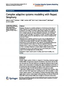
List of Figures 2.1
Simple Electrical Circuit . . . . . . . . . . . . . . . . . . . . . . . . . . . 27
3.1
A Heat Plate . . . . . . . . . . . . . . . . . . . . . . . . . . . . . . . . . . 46
3.2
A Simple Truss . . . . . . . . . . . . . . . . . . . . . . . . . . . . . . . . 49
3.3
Simple Electrical Circuit . . . . . . . . . . . . . . . . . . . . . . . . . . . 54
3.4
Class Diagram for Circuit Example . . . . . . . . . . . . . . . . . . . . . . 56
3.5
Snapshot of CUML tool with Class Diagram for Circuit Example . . . . . . 57
3.6
Popup window for entering/editing constraints and other specifications of a Class . . . . . . . . . . . . . . . . . . . . . . . . . . . . . . . . . . . . . 57
3.7
Popup Window through which the constructor of a class can be defined/edited. 58
3.8
Snapshot of CUML tool showing the Cob code generated from the Class Diagram of Figure 3.5. . . . . . . . . . . . . . . . . . . . . . . . . . . . . 59
3.9
Snapshot of the Truss Drawing Tool showing a Sample Truss . . . . . . . . 61
3.10 Popup Window for Entering Values for Attributes of a Beam . . . . . . . . 62 4.1
Algorithm for renaming variables . . . . . . . . . . . . . . . . . . . . . . . 81
4.2
Cob Class Definitions . . . . . . . . . . . . . . . . . . . . . . . . . . . . . 83
4.3
Translated CLP Program . . . . . . . . . . . . . . . . . . . . . . . . . . . 84
5.1
Cob Computational Environment: build phase . . . . . . . . . . . . . . . . 103
5.2
Cob Execution Environment: solve phase . . . . . . . . . . . . . . . . . . 104
5.3
Cob Interactive Execution Environment . . . . . . . . . . . . . . . . . . . 105
5.4
Cob Execution Environment: query phase . . . . . . . . . . . . . . . . . . 106
5.5
Cob class definitions . . . . . . . . . . . . . . . . . . . . . . . . . . . . . 113
5.6
Translated CLP(R) code . . . . . . . . . . . . . . . . . . . . . . . . . . . 114 ix
5.7
Scheme for Partial Evaluation . . . . . . . . . . . . . . . . . . . . . . . . 122
5.8
Constraints obtained by partial evaluation of samplecircuit . . . . . . . . . 124
5.9
Object Graph of Samplecircuit . . . . . . . . . . . . . . . . . . . . . . . . 132
6.1
A Separation Flow Sheet . . . . . . . . . . . . . . . . . . . . . . . . . . . 141
6.2
Sample Graph. . . . . . . . . . . . . . . . . . . . . . . . . . . . . . . . . 157
6.3
Naive evaluation of a relaxation goal. . . . . . . . . . . . . . . . . . . . . 160
7.1
Snapshot of the Circuit Drawing Tool . . . . . . . . . . . . . . . . . . . . 173
7.2
Snapshot of the input window for a resistor in the circuit drawing tool . . . 174
7.3
Snapshot of the Circuit Drawing Tool showing input and output windows and details of resistor . . . . . . . . . . . . . . . . . . . . . . . . . . . . . 175
7.4
Snapshot of the Analog Circuit Drawing Tool . . . . . . . . . . . . . . . . 176
7.5
Gear Train as Constrained Objects . . . . . . . . . . . . . . . . . . . . . . 181
7.6
Structure of a Simple Book . . . . . . . . . . . . . . . . . . . . . . . . . . 189
8.1
A Simple Truss . . . . . . . . . . . . . . . . . . . . . . . . . . . . . . . . 225
x
Abstract This dissertation investigates the theory, design, implementation and application of a programming language and modeling environment based on the concepts of objects, constraints and visualization. We focus on modeling complex systems that can be described as an assembly of interconnected, interdependent components whose characteristics may be governed by laws, or constraints. Often, a natural visual representation can be associated with each of the components and their assembly. Such complex systems occur in a wide variety of domains such as engineering, biological sciences, ecology, etc. Modeling such systems therefore involves the specification of their structure and behavior, and also their visualization. In modeling structure, we can think of each component as an object, with internal attributes that capture the relevant features. In modeling behavioral laws or invariants, it is natural to express them as constraints over the attributes of an object. When such objects are aggregated to form a complex object, their internal attributes might further have to satisfy interface constraints. The resultant state of a complex object is deduced by satisfying the internal and interface constraints of the constituent objects. This paradigm is referred to as constrained objects. We describe a principled approach to the design of a constrained object programming language built on rigorous semantic foundations. Our proposed language, Cob, provides a rich set of modeling features, including object-oriented concepts such as classes, inheritance, aggregation and polymorphism, and also declarative constraints, such as symbolic, arithmetic equations and inequalities, quantified and conditional constraints, and disequations. We define the semantics of constrained objects based upon a translation to constraint logic programs (CLP). A Cob class is translated to a CLP predicate and the set-theoretic semantics of the class are given in terms of the least model of the corresponding predicate. Such semantics also pave the way for a novel implementation of constrained objects. However, due to the limitations of CLP, such an implementation cannot handle conditional constraints and may not give satisfactory performance for large-scale models. To overcome these limitations, we have developed partial evaluation techniques for generating
optimized CLP code. These techniques also allow us to use our own handler for evaluating conditional constraints, and employ a more powerful existing solver for handling complex non-linear constraints. Based on partial evaluation, we have developed novel techniques for interactive execution of Cob models and fault detection in over-constrained structures. Often a constrained object model of a complex system may have more than one solution. We allow the modeler to state preferences within a Cob class definition and the resultant state of the system is obtained by constraint solving and optimization. The semantics of Cob programs with preferences are based upon a translation to preference logic programs (PLP). We also investigate different forms of relaxation of preferences to obtain suboptimal solutions and propose a scheme for the operational semantics of relaxation that accounts for recursively defined PLP predicates. We give several examples from different domains to illustrate that the paradigm of constrained objects provides a principled approach to modeling complex systems and is amenable to efficient and interactive execution.
ii
Chapter 1 Introduction 1.1
Motivation and Significance
This dissertation investigates the theory, design, implementation and application of a programming language and modeling environment based on the concepts of objects, constraints, and visualization. Our focus is on modeling systems that consist of an assembly of interconnected, interdependent components that have the following characteristics: 1. They are compositional in nature, i.e., a complex structure is made of smaller structures or components which are further composed of smaller components and so on. 2. The behavior of a component by itself and in relation to other components is generally governed by some laws or rules. 3. There is a natural visual representation that can be associated with each component. Examples of such systems occur in different domains: engineering, organizational enterprises, biological systems, ecosystems, business processes, information warehouses, and program execution. One of the main goals of our research is to provide a modeling environment that facilitates a principled approach to modeling such complex systems. Such an environment should facilitate intuitive creation and manipulation of models that are easy to understand, modify and debug. We also require that, where appropriate, a model should be given a visual representation. Thus the modeling environment for complex systems should 1
facilitate compositional specification of structure, declarative specification of behavior, and visual development and manipulation of models (where appropriate). In modeling structure, it is natural to adopt a compositional approach since a complex engineering entity is typically an assembly of many components. In programming language terms, we may model each component as an object, with internal attributes that capture the relevant features that are of interest to the model. The concepts of classes, hierarchies and aggregation found in object-oriented (OO) languages, such as C++, Java, and Smalltalk, are appropriate to model the categories of components and their assembly. However, in modeling the behavior of complex engineering entities, the traditional OO approach of using procedures (or methods) is inappropriate because it is more natural to think of each component as being governed by certain laws, or invariants. Using methods to represent behavioral laws places the responsibility of enforcing them on the programmer. Moreover, these laws become implicit in the procedural code, instead of being explicitly declared. From a programming language standpoint, it is more natural to express behavioral laws as constraints. A constraint is a declarative specification of a relation between variables/attributes. Constraint programming languages are declarative in that the programmer specifies what constraints define the problem without specifying how to solve them. The constraints and their solving techniques are appropriate to model, test and enforce (solve) the behavioral constraints of a system. Constraints thus facilitate a declarative specification of the behavior of a complex system. However, a pure constraint programming language does not provide an adequate representation for the structure of a system. It lacks the modularity of object-oriented languages, and a complex system appears as a large collection of constraints with little correspondence to the structure of the system being modeled. A more direct and intuitive approach to modeling is through a visual representation of the system in the form of two or three dimensional drawings. A visual representation can be easier to understand since it is less abstract and bears close physical resemblance to the real system. For example, engineering drawing tools provide a convenient way for a modeler to visualize and design a structure. Such visualization of a structure though proportional and drawn to scale, is however a purely geometric representation. It captures the geometric attributes of the structure and but does not have any correlation to the underlying semantics.
2
For example, one may draw a sketch of a bridge, but there is no way to infer its load bearing capacity etc. from the drawing. Thus, while the paradigms of objects, constraints, and visualization each offer features suitable for modeling certain aspects of a complex system, they are individually inappropriate for modeling both the structural as well as behavioral aspects of the system. In this dissertation we investigate the theory, design and implementation of a programming language and modeling environment based on the notion of constrained objects. This approach combines the modular aspects of objects with the declarative nature of constraints, and, together with visualization, provides a powerful modeling environment for complex systems.
1.2
Objectives and Results
1.2.1 Technical Approach A constrained object is an object whose attributes are governed by laws or declarative constraints. When such objects are aggregated to form a complex object, their internal attributes might further have to satisfy interface constraints. In general, the resultant state of a complex object can be deduced only by satisfying both the internal and the interface constraints of the constituent objects. This paradigm of objects and constraints is referred to as constrained objects, and it may be regarded as a declarative approach to object-oriented programming. To illustrate the notion of constrained objects, consider a resistor in an electrical circuit. Its state may be represented by three variables V, I, and R, which represent respectively its voltage, current, and resistance. However, these state variables may not change independently, but are governed by the constraint V = I * R. Hence, a resistor is a constrained object. When two or more constrained objects are aggregated to form a complex object, their internal states may be subject to one or more interface constraints. For example, if two resistor objects are connected in series, their respective currents should be made equal. Similarly, in the civil engineering domain, we can model the members and joints in a truss as objects and we can express the laws of equilibrium as constraints over the various forces 3
acting on the truss. In the chemical engineering domain, constrained objects can be used to model mixers and separators, and constraints can be written to express the law of mass balance. In the paradigm of constrained objects that we present, a complex object may also have a visual representation, such as a diagram. This visual representation is compositional in nature; that is, each component of the visual form can be traced back to some specific object in the underlying constrained object model. An end-user, i.e., modeler, can access and modify the underlying model using the visual representation. This capability may be contrasted with currently available tools for engineering design such as AutoCAD, Abaqus, etc., where the visual representation contains only geometric information but does not provide access to the underlying logic or constraints. We expect to have different visual interfaces for different domains but a common textual language (described in Section 3) for defining the classes of constrained objects. We expect a modeler to first define the classes of constrained objects, by specifying their attributes and their internal and interface constraints. These classes may be organized into an inheritance hierarchy. Once these definitions have been completed, the modeler can build a specific complex object, and execute (solve) it to observe its behavior. This execution will involve a process of logical inference and constraint satisfaction [32, 33, 40, 49, 59]. A modeler will then need to go through one or more iterations of modifying the component objects followed by re-execution. Such modifications could involve updating the internal states of the constituent objects, as well as adding new objects, replacing existing objects, etc. The complex object can be queried to find the values of attributes that will satisfy some given constraints in addition to the ones already present in the constrained objects.
1.2.2 Scope of the Dissertation We describe below the major areas of investigation along with a brief summary of our contributions within these areas.
4
Language Design. We develop a novel programming language, Cob, based on the notion of constrained objects. The language facilitates declarative specification of a wide variety of constraints including arithmetic and symbolic. We provide quantified constraints for compact specification of a relation whose participants may range over enumerations, i.e., indices of an array or the elements of an explicitly specified set. Similarly, we also provide a notation for iterative terms appearing in arithmetic constraints. Such a declarative syntax brings the constraint specification closer to its mathematical equivalent. We also provide conditional constraints, which are a powerful and expressive means of stating different constraints depending on the state of a constrained object. We also allow user-defined predicates within a constrained object class definition and give several examples illustrating the use of these constructs and the application of Cob to modeling problems from various domains. Modeling Environment. We provide two types of visual interfaces for the creation of constrained object models, their modification and execution. A domain independent visual interface is provided for authoring constrained object class diagrams. The definition of a constrained object class (i.e., its attributes, constraints, constructors etc.) and its relation (e.g. inheritance, aggregation, etc.) to other classes can be specified through a graphical user interface. The interface can be used to run (solve) the constrained object model and query it for values of attributes. We also provide different domain dependent visual interfaces for drawing constrained object models of engineering structures such as electrical circuits and trusses. These diagrams of engineering structures can themselves be thought of as programs since they can be created, modified and executed through this visual interface which also displays answers (values of attributes) to queries. Formal Semantics.
We define formal declarative and operational semantics for con-
strained objects. The formal semantics of a programming language provide a mathematical model for its programs and can be used for its analysis e.g. computability, verification, etc. A constrained object can be understood as an abstract datatype whose characteristics are described axiomatically through constraints. Informally, the meaning of a constrained object is the set of values for its attributes that satisfy its constraints. We define a set-theoretic 5
semantics of constrained objects that is based on a mapping between constrained objects and constraint logic predicates [59, 60]. The operational semantics are given as rewrite rules and serve as a basis for an implementation of the constrained object paradigm. Execution Environment. We provide an implementation for constrained objects based on a translation to the constraint logic programming language CLP(R). A class is mapped to a CLP(R) predicate such that the constraints of the class form the body of the predicate. In this way the predicate serves as a procedure that enforces the constraints. However, due to the limitations of CLP(R), such a translation alone cannot satisfactorily handle conditional and non-linear constraints and may also be inefficient for large models. Therefore, we have developed techniques for partial evaluation of constrained object programs that generate optimized code and facilitate handling of conditional constraints, and deployment of more powerful constraint solvers for non-linear systems of constraints. Partial evaluation also facilitates efficient re-solving when a model is modified. Using partial evaluation, we have developed techniques for visual interactive execution and debugging of a constrained object program based on its object structure. For a given instance of a complex constrained object, its object structure represents the relation between the instances of its components. Preferences and Relaxation. When a system of constraints has more than one solution, there may be a preference for one solution over another. For such cases, we extend the syntax and semantics of constrained objects to allow the specification of constraint optimization problems. Two forms of optimization are provided: maximization (or minimization) of an arithmetic function and the more general form of a preference clause [38]. The semantics of constrained object programs with preferences are based on a mapping to preference logic programs (PLP) [38]. When preferences are specified in a constrained object class definition, we determine the set-theoretic semantics of the class from the set of preferential consequences of the corresponding predicate. Often, one may be interested in the optimal as well as suboptimal solutions to an optimization problem. This requires a relaxation of the preference criteria and we explore different forms of relaxation: with respect to the underlying preference criterion or with respect to an extra constraint. We address the computational problems arising from relaxation 6
and provide an intuitive operational semantics for relaxation goals in PLP. Applications. We present several examples throughout the dissertation to illustrate that the paradigm of constrained object is appropriate for modeling complex systems from various domains. We present three case studies that describe the constrained object methodology for modeling complex systems which gives a compositional specification of the structure and declarative specification of the behavior of the system. The ability to specify, run, query, and debug partial models, textually as well as through graphical user interfaces, makes the constrained object paradigm useful in general and also for pedagogical purposes in the engineering domain. This dissertation presents a novel programming language and modeling environment called Cob based on the notion of constrained objects and their visualization that facilitates a principled approach to the modeling of complex systems.
1.3
Summary of Dissertation
The remainder of this dissertation is organized as follows. Chapter 2 gives an overview of constraints and constraint programming techniques. The paradigms of constraint (logic) programming and preference logic programming are described in detail along with several examples. Chapter 3 gives the syntax of the constrained object programming language named Cob, and describes its modeling environment. Several examples are given to illustrate the use and application of the various constructs of this language and environment. Chapter 3 also gives a comparison with related work. Chapter 4 describes formal declarative and operational semantics of constrained objects. Chapter 5 discusses implementation techniques for constrained objects. This includes the translation to CLP(R) and a scheme for partial evaluation. Chapter 6 gives a description of the extension of the constrained object paradigm to handle optimization problems and discusses the computational issues of relaxation in preference logic programs. Chapter 7 presents case studies illustrating the development and application of constrained object models in different domains. Chapter 8 gives conclusions and our current and future research plans.
7
Chapter 2 Background This chapter presents an overview of some basic concepts and computational techniques relating to constraints and constraint programming languages. Two constraint programming paradigms are discussed: constraint logic programming and preference logic programming. The work on constrained objects presented in this dissertation is closely related to these two programming paradigms. The overview presented in this chapter provides the necessary background for understanding the rest of the dissertation.
2.1
Constraint Programming
The overview of constraint programming presented in this section is summarized from [81, 8, 9, 70] and from [51] which gives a comprehensive survey of constraint programming.
2.1.1 Constraint A constraint is a relation among variables and serves to specify the space of possible values for these variables. For example, the equation X
Y �
0 is a constraint that restricts the
values of variables X and Y to add up to a positive number. A constraint may involve arithmetic, relational, boolean and set operations. Following are the main characteristics of constraints. �
A constraint is a declarative specification of a relation between variables, but does not specify any algorithm or procedure to enforce the relation. 8
Constraints are non-directional, i.e., they do not have input/output variables. The �
same constraint X
Y
Z may be used to compute both the constraints on X given
the constraints on Y and Z as well as the constraints on Z given the constraints on X and Y . Due to their declarative and non-directional nature, the order of constraints does not �
matter. A constraint may give partial information relating a variable to other variables or �
values, or it may specify its exact value(s). Constraints are additive, i.e., a constraint may be added to an existing store of con�
straints, and the conjunction of all existing constraints is required to hold simultaneously. It is possible that the addition of a constraint makes the constraint store inconsistent. This is referred to as an over-constrained system and is discussed later in Section 2.1.3. �
A constraint domain refers to the data domain of each variable and the operations and relations defined on these domains. Different variables can have different domains.
Problems in the areas of engineering modeling, operations research, combinatorics, databases, information retrieval, user interface construction and document formatting are often characterized by relations such as: laws of physics (e.g. balance of forces, conservation of mass and energy), functional specifications (e.g. input-output torque, power), performance requirements (e.g. efficiency, speed), scheduling restrictions (e.g. availability, feasibility, preference), data integrity (e.g. an employee’s salary should be consistent with his grade), etc. A declarative specification of constraints facilitates a natural and intuitive description of such problems.
2.1.2 Constraint Satisfaction A constraint satisfaction problem (CSP) consists of a finite set of variables, a domain (of values) for each variable, and a finite set of constraints involving these variables. A
9
solution to a CSP is a valuation, or mapping, of its variables to values in their respective domains that satisfy all the constraints of the CSP. The goal of a constraint satisfaction algorithm is to determine whether a solution exists, and to find one or more or all solutions to the constraints. In the case of multiple solutions, the goal might be to find an optimal solution with respect to a given objective (cost) function. Constraint satisfaction algorithms can be broadly divided into two categories based on the domains of the variables. Finite Domain CSP. Satisfaction techniques for CSP over finite domains are combinatorial in nature and we describe some of these techniques here. The following description is summarized from [51, 8, 9] and [70] which gives a comprehensive survey of constraint satisfaction algorithms for finite domains. Algorithms for finite domain CSP include those based on search, inconsistency detection or stochastic methods. A simplistic search algorithm that can solve any finite domain CSP is the generate-and-test (GT) scheme. This scheme generates combination of values for the variables, and tests the constraints for these values. This scheme is inefficient since it may generate every possible combination. A relatively efficient search technique uses backtracking (BT). Here, variables are sequentially instantiated with values from their domain. Each time a variable is instantiated the pertinent constraints are tested. If a constraint fails, the system backtracks to pick an alternate value for the most recently instantiated variable having alternatives. Thus, when a constraint fails, this scheme prevents the generation of a subset of combination of values that are guaranteed to fail. Although more efficient that GT, for most non-trivial problems, backtracking takes exponential time. Constraint satisfaction algorithms based on inconsistency detection use the notion of a constraint graph to reduce backtracking while searching for a solution. The nodes of this graph represent distinct variables and there is an edge between two variables if they appear in a single constraint. A unary constraint is represented as an edge from a node to itself. Since any finite domain CSP can be mapped to an equivalent CSP in which every constraint has at most two variables [94], it suffices to discuss only binary CSP. Some basic consistency based algorithms use: (i) node consistency: remove those values from a variable’s domain that violate any unary constraint involving the variable; (ii) arc 10
consistency: remove those values from a variable’s domain that violate a constraint on that variable; (iii) path consistency: remove pairs of values that satisfy a constraint (edge) but do not satisfy a series of constraints that form a path between the variables. Neither node nor arc consistency for a set of constraints however, implies their solvability. A stronger notion of k-consistency, based on path consistency, has been defined which ensures that any partial solution/instantiation of k
1 variables which does not violate any
constraints can be extended by the instantiation of any kth variable such that the constraints are still not violated. A constraint graph is strongly k-consistent if it is j-consistent for all j �
k [70]. Node consistency is equivalent to strong 1-consistency; arc consistency is equiv-
alent to strong 2-consistency; and path consistency is equivalent to strong 3-consistency. Algorithms based on k-consistency take a partial solution and try to extend it to a full solution. If a constraint graph with n variables is strongly n-consistent then it is solvable without any backtracking. But making an n-node constraint graph strongly n-consistent can take exponential time in the worst case. Hence, more practical approaches try to make the constraint graph strongly k-consistent for k �
n. The aim of these algorithms is to make the
search for a solution backtrack-free. These algorithms combine simple backtracking with arc consistency, i.e., in every step of the backtracking algorithm, they try to make the graph arc-consistent. Every time a variable is instantiated, consistency check is performed on uninstantiated variables. There are different algorithms depending upon the extent of this checking: forward checking (FC), partial lookahead (PL), full lookahead (FL) and really full lookahead (RFL). These algorithms are called constraint propagation algorithms since they propagate information about one constraint to another. We have discussed only some of the interesting techniques for finite domain CSP above. Other techniques include stochastic methods [86], algorithms that exploit the structure of the problem [21], and identifying tractable classes of problems [31, 78, 22]. Non-finite Domain CSP. The solving techniques for CSP in which the variables may have an infinite domain are usually mathematical or numeric-based, e.g., the Gauss-Jordan elimination method, Newton method, Taylor series, Kachian and Karmarkar, Simplex algorithm or automatic differentiation. Constraint solving techniques for infinite domain are often specialized for a particular domain (e.g. real or rational numbers) as well as cate11
gory of constraints (e.g. linear, non-linear or differential equalities or inequalities). The generality of the solving algorithm is a tradeoff with its efficiency. Typically, a constraint solving system keeps the constraints in a standard canonical form ,e.g., X �
such as Xi
0, X bi
�
0 or ∑ni 1 ci Xi
� ������
ci1 Ti1
d. Equations are maintained in parametric solved form
�
cin Tin , where Xi is a non-parametric variable and Ti j s are
parametric variables [62]. Common steps in a basic algorithm for solving linear equality constraints such as Gaussian elimination involve substitution of parametric variables by equivalent parametric expressions. When sufficient information about (parametric) variables is obtained, the values of the non-parametric variables can be computed. Inequality solvers may also maintain constraints in a solved form and determine implied equalities from the set of inequalities. When used in a constraint programming system such algorithms are adapted to be incremental, performing substitution and pivoting operations to get back the canonical form after constraints are added. Some constraint solving techniques for linear equality and inequality constraints are described in [63, 75, 48, 56].
2.1.3 Programming with Constraints Computing with constraints involves the specification, generation, manipulation, testing and solving of constraints. A computational system based on constraints provides a syntax for specifying, combining and manipulating constraints and its underlying computational engine provides mechanisms for processing, testing and solving constraints. The computational engine may use inference, backtracking, search, constraint propagation, entailment and/or optimization techniques for constraint satisfaction. A majority of constraint programming (CP) systems are based on the syntax and control mechanism of logic programming, e.g., constraint logic programming [59, 61] and concurrent constraint programming [99]. Other CP systems combine constraints with imperative programming, functional programming and term rewriting. We give a brief overview of these major categories of constraint programming languages which are described in [81]. Constraint Logic Programming. Constraint logic programming (CLP) merges constraints into the framework of logic programming. A CLP system is characterized by its constraint
12
domain and the solver for that domain. Unification between terms is generalized to constraint solving over the data domain. CLP languages can be used to model a wide variety of problems including arithmetic, scheduling, as well as combinatorial problems and constraints can be used to prune the space of solutions. There are numerous constraint logic programming languages for modeling problems and solving constraints over different domains. For example, the CHIP [24] language provides boolean, linear constraints and finite domain constraints. The clp(FD) solver [16] provides finite domain constraints and is used for discrete optimization and verification problems like scheduling, planning, etc. The CLP(R) [58] language provides constraints over real numbers but solves only linear constraints. Our work on constrained objects is directly related to the CLP paradigm. In Section 2.2, we describe the CLP paradigm and the CLP(R) language in some detail. Concurrent Constraint Programming. Concurrent constraint programming merges constraints into the framework of concurrent logic programming [100]. A rule defines a “process” and comprises of guard conditions, or constraints, and a body which is a sequence of literals. A rule can be used to resolve a goal if its guard conditions are enabled. The guard conditions can be of two kinds: ask and tell. The former checks for entailment while the latter (checks for compatibility and) adds the constraint to the current constraint store. The evaluation mechanism CCP programs differs from CLP programs in that if more than one rule can be used to reduce the goal, then any one is picked randomly. The evaluation scheme does not consider any other rules (enabled or not enabled) at any later stage. Concurrent constraint programming is used for modeling reactive systems, e.g. incremental constraint solvers. Some concurrent constraint programming languages are cc(fd) [50], Oz [105], AKL [65], CIAO [52]. Constraint Handling Rules. Constraint handling rules (CHR) [35, 36] are a high-level language designed specifically for writing constraint solvers. They consist of multi-headed guarded rules which are used to rewrite a constraint store (a set of constraints). Constraints that match the left hand side of a rule can be replaced by the constraints on the right hand side of the rule if the guard is implied by the constraint store. Applying a CHR can result in simplification of constraints or propagation. Simplification replaces constraints with 13
simpler equivalent constraints while propagation adds a new redundant constraint that may cause further simplification. The constraint store is manipulated by repeatedly applying the constraint handling rules until further application does not change the constraint store. CHRs can be used to build new constraint solvers, extend existing ones with new constraints, specialize constraint solvers for a particular domain or application or combine constraint solvers. CHRs can be combined with a high-level host language (e.g. CLP) to define user-defined constraints and constraint solvers. Constraints + Object-Object Programming. Languages such as Kaleidoscope [76, 75], Siri [55], ThingLab [10], Modelica [34] integrate constraint into an object-oriented framework. In ThingLab, each constraint is accompanied by methods for solving it and the system arrives at a constraint satisfaction plan using the appropriate method. Siri simulates imperative constructs through “constraint patterns” [54]. In Modelica there is a clear separation between constraints and imperative constructs which can both exist in a class definition. Kaleidoscope simplifies user-defined constraints until a primitive constraint solver can be used to solve them. We give a detailed comparison of our work with these languages in Section 3.4. Constraints + Term Rewriting.
Term rewriting is a declarative paradigm that uses rewrite
rules along with pattern matching to simplify terms. If an expression matches the left hand side of a rewrite rule, it can be replaced by the expression on the right hand side of the rule. For example, one can define rewrite rules to express any Boolean formula in conjunctive normal form. Augmented term rewriting in Bertrand [72] combines constraints with term rewriting. Augmented term rewriting extends term rewriting by providing substitution of a variable by an expression and the introduction of new local variables on the right hand side of a rule. In an augmented term rewriting system, there is no global constraint store or solver, since the rewrite rules themselves are used to define constraint solving. Another approach to combining constraints with term rewriting provides conditional rules or rules with guard conditions: rules that are applicable only when their constraint or guard condition is true. Such systems are typically used to implement automatic theorem provers [57, 6] and are considered closer to CCP than to CLP [81]. 14
Constraints + Functional Programming. There have been three major approaches to combining constraints with functional programming [81]. A simple approach is to treat constraints as functions that return answers. However, these are not constraints in the declarative sense since the programmer must provide the functions for solving the constraints. Another approach is to embed functions in a constraint language like CLP. Although built-in functions such as +, -, etc. are provided in CLP, the system should also allow user-defined functions. Treating functions as relations with an extra argument representing the result is not sufficient since the system does not have enough knowledge to reason about such functions when they appear in constraints. By knowledge, we mean properties like associativity, commutativity, etc. Also multi-directional evaluation of functions might not always be possible. A third approach treats functions and constraints to be at the same level and extends lambda calculus with a global constraint store. One such approach called constrained lambda calculus [79] uses the constraint store to determine value of variables. Another approach in the language Oz [105] (which has constraint solvers for tree constraints and finite domain constraints) associates guard constraints or conditions with lambda expressions and variables may range over lambda expressions (functions). Constraint Solving Toolkits and Symbolic Algebra Packages. Constraint solving toolkits such as JSolver (Java solver), ILOG solver [91] or 2LP [5] embed a solver into an imperative host language. The programmer can access the solver only through an interface. Such toolkits are usually specialized for a particular domain of problems. Symbolic algebra packages such as Matlab [109], Maple [112], MACSYMA [43], Mathematica [115] are mathematical languages typically used by scientists and mathematicians to solve simultaneous linear, non-linear or differential, equations, inequalities, etc. These are powerful tools that can solve or simplify a system of mathematical constraints. Some of them have some programming facilities but little by way of controlling the solving. Over-Constrained Systems. A system of unsatisfiable constraints is called an over-constrained system. The study of over-constrained systems includes developing techniques for detecting an over-constrained system, locating the cause of the error and relaxing some constraints in order to get a solution. Over-constrained systems are less likely to occur when a 15
constraint may be tagged as a “soft” constraint [113], i.e., it is not required to be satisfied. One approach to specifying a soft constraint is to associate a strength or weight with each constraint and to specify an error function which associates an error with a constraint and a valuation and can be used to compare alternate valuations [113]. Intelligent backtracking in CLP detects independent subgoals in a query. These goals can be run in parallel [7] because an error cannot be caused by their interaction. Among other reasons, the study of over-constrained systems is motivated by problems of belief revision in artificial intelligence, where a new belief may contradict an existing belief set [37, 83]. A technique for detecting a contradictory set of constraints is given in [18]. This technique is for linear equalities and inequalities, and it is based on introducing an extra error variables into constraints and then solving to minimize their sum. The constraint whose error variable gets a non-zero value is removed because it is considered unsatisfiable and the process is redone. In the end a minimal set of unsatisfiable constraints is obtained. A collection of articles on over-constrained systems appears in [64]. Constraint Optimization.
It is often the case that a set of constraints has more than one
solution. In such cases there may be a criterion based on which one solution can be declared to be better than another. This criterion is referred to as the optimization or preference criterion. The problem then is to determine the optimal solutions from a set of feasible solutions based on this criterion. The preference criterion may be used to rank multiple solutions in decreasing order of preference and the top ranking solutions are optimal. In general, however, the preference criterion may not be able to place all the solutions in a total order. The most well-known optimization technique is linear programming. A set of linear constraints over some variables is given which may include the range of the variables. Also given is a mathematical function involving some or all of these variables. This function is called the objective function, and the goal is to find a solution to the constraints that minimizes or maximizes the objective function as the case may be. Another way to state an optimization problem is to specify a set of constraints and indicate which ones must be satisfied and which ones may be violated if it is not possible to satisfy them all. The hierarchical constraint logic programming (HCLP) language [11, 113] 16
incorporates the notion of constraint hierarchies into the CLP paradigm. Constraints can be tagged required, strong, medium, weak, etc., and the computational engine tries to first find a solution that satisfies all the required constraints, and then as many of the strong constraints, and subsequently as many of the medium constraints, and so on as possible. A more general language for expressing constraint hierarchies and constraint optimization within the realm of constraint logic programming is the preference logic programming (PLP) paradigm [38]. We discuss it in more detail in section 2.3.
2.2
Constraint Logic Programming
The Constraint logic programming (CLP) [59, 61] scheme is a merger of two declarative paradigms: logic programming and constraint programming. Logic programming emerged from research in resolution theorem proving and artificial intelligence. A basic logic program is a set of Horn clauses (a subset of first order logic) and the goal or query to be proved is also a special kind of Horn clause (headless). The observation that logic programming is basically a kind of constraint programming where the constraints are equalities over terms and constraint-solving is term-unification led to the development of constraint logic programming. CLP extends logic programming with constraint solving capabilities and generalizes unification to solvability over the constraint domain. At the core of a CLP scheme lies a structure. Informally, a structure is a domain comprising a set of values along with functions and relations on this set. The relations can be thought of as constraints. The structure must be solution compact, i.e., it should be possible to describe every value in the domain by a conjunction of a (possibly infinite) set of constraints and the complement of every constraint should be definable as a disjunction of a (possibly infinite) set of constraints [61]. Given the CLP scheme and a constraint domain, we get an instance of a CLP language. For example, clp(FD) represents constraint logic programming over finite domain constraints; CLP(R) is the constraint logic programming language over the real number domain; clp(B) is a constraint logic language with boolean constraints. CLP(Term), where Term is the traditional logic terms with unification, represents the Prolog-like logic programming paradigm. Our paradigm of constrained
17
objects bears close relations with the CLP(R) scheme and hence we give an overview of the CLP(R) language next.
2.2.1 The CLP(R) Language The syntax and computational model of the CLP(R) language bear close resemblance to those of traditional logic programming languages such as Prolog. We describe CLP(R) by highlighting the generalizations it makes to logic programming. This description summarizes a more detailed discussion given in [44, 63]. Syntax. We describe the syntax of CLP(R) terms, constraints and rules. Term. �
A term can be a variable, constant, or an arithmetic expression involving
variables, real number constants or functions such as sin, cos, etc. As in logic programming, terms are built from constants and uninterpreted functors, i.e., if t 1 �
are terms and if f is an uninterpreted functor, then f t1 Explicit Constraint. �
The relational operators (
����� tn
is a term. �
�
�
�
����� tn
) over the real number
domain are used to form explicit constraints. Note that explicit constraints cannot involve uninterpreted constants or functors. Equality between uninterpreted functor terms is treated as unification. Goal. A goal is similar to a Prolog goal except that it can have explicit constraints. �
Thus, a goal is a sequence of literals and explicit constraints. A literal is a positive or a negative atom or explicit constraint. If p is an n-ary predicate symbol and t 1 are terms then p(t1 �
Rule.
����� tn) is an atom [73].
����� tn
A rule is similar to a Prolog rule except that the atoms in the body of a rule
can be explicit constraints. Thus, a CLP(R) rule is of the form A :- B where A is an atom and B is a goal. A fact is a rule with an empty goal as the body. A CLP(R) program is a sequence of rules. A CLP(R) query is a goal and it is evaluated with respect to a CLP(R) program. We describe goal evaluation next.
18
Goal Evaluation. As mentioned earlier, unifiability amongst terms in logic programming is generalized to solvability of constraints over R, the real number domain, in CLP(R). The evaluation of a goal with respect to a CLP(R) program works along the lines of goal resolution in a logic programming context. We provide an informal description here; a formal description of a CLP(R) program, a query and resolution with the declarative and operational semantics is given in Section 4.1. The evaluation of a goal G0 with respect to a CLP(R) program P can be described in terms of a derivation or a finite sequence of states S0 Gi
���
�����
Sn . A state Si is represented as
Ci � where Gi is a goal and Ci represents a collection of constraints or a constraint
store. Solution. �
A set of constraints is solvable if there exists a mapping from their
variables to values in R such that the constraints evaluate to true. The mapping is called a solution to the constraints. Constraint Solver. A constraint solver tests whether a given set of constraints can �
be solved. It may also find a solution to the constraints and/or simplify them. Typically, a constraint solver is built for a specific domain. In the CLP(R) context, the constraint solver is used to solve the conjunction of arithmetic constraints present in the constraint store over the real number domain. Typically such a constraint solver will perform incremental constraint solving since the constraint store is expected to change (add or delete constraints). The properties of the domain (in this case the real number domain R) are built into the constraint solver so that it does not have to perform generate-and-test in order to solve/test constraints. For example, the CLP(R) constraint solver can deduce that the conjunction of the constraints X and X �
�
Y
Y is false without testing the constraints for any particular values. In other
words, the solver has the ability to reason about one or more constraints using its knowledge about the domain and the built-in operations on this domain. The solver uses an adaptation of the Two-Phase Simplex algorithm and [103] for deciding linear
�
inequalities and Gaussian Elimination for linear equalities. Derivation. Given a query G0 and a CLP(R) program P, a derivation of G0 with 19
respect to P is a sequence of states S0
G0
���
�����
true � S1 S2
with the following
properties. – Start State. The start state (S0 ) of a derivation consists of the goal G0 and an empty constraint store. – Derivation Step. A state Si
�
Gi
1
the following holds. Let Gi
�
Ci
�
is derived from Si
����� Am and suppose A j ( j � 1 ��� m
A1
1
���
1�
for resolving. There are three cases: 1. A j is an atom: Suppose it is of the form p(t1
� ����� t � ) n
P of the form p(t1
����� n B A j� 1
� t
�
Am and Ci
:- B then Gi
�
1
Gi ��� Ci � if �
is selected
����� tn). If there is a rule in � ����� t ����� A 1 A j � 1 t1 t1 n
Ci . Note that before this step is applied, the
1
variable of the pertinent rule of P are renamed to remove any common variable names between the goal and the rule. If there does not exist such a rule in P, then Si
�
φ
1
���
f alse � .
2. A j is an explicit constraint: It is added to the constraint store and hence Gi
�
����� A j � 1 A j� 1 �����
A1
1
Am and Ci
�
1
Ci
��� A j � .
3. A j is a unification constraint (term equality): Such equations are between non-arithmetic terms and may or may not involve functors. This is similar to the term equality in standard logic programming and is handled by a unification algorithm. Note that this may give rise to explicit (equality) constraints if arithmetic subterms are present. Equality between an arithmetic and non-arithmetic term results in the state Si
�
1
φ
���
f alse � .
– At every step of the derivation, the constraint store is checked for consistency. �
If Si then Si
�
Gi 1
���
Ci � and solv Ci φ
���
�
f alse, i.e., the constraint store is inconsistent,
f alse � . If the constraint store is consistent, then the derivation
�
proceeds to the next step. Successful Derivation. A derivation is said to be successful if it is finite and its final state consists of an empty goal and a consistent constraint store. There can be more than one successful derivation.
20
Answer Constraint. �
The concept of answer substitution in logic programming is
generalized to an answer constraint in CLP(R). The constraints in the constraint store at the end of a successful derivation form the solution to the goal. Specifically, the restriction of these constraints to those containing variables from the initial goal are the answer constraints, or the computed answer. Multiple successful derivations could give rise to multiple computed answers. Every instance of the answer constraint is a solution. Finitely Failed. If all the derivations for a goal are finite and end in failure, then the �
goal is said to have finitely failed, i.e., there is no computed solution. CLP(R) System. We now give some practical details of a CLP(R) system [58]. The literal selection strategy in the basic CLP computational model is impartial, mak�
ing solutions independent of goal ordering. However, a practical implementation invariably deviates from this strategy in the following ways: 1. The atoms in a goal are selected in a left-to-right order. A programmer can write more efficient programs by placing subgoals that test constraint satisfaction before those that generate solutions. We explain this point later with an example. 2. The goal selection between a parent subgoal and child subgoal follows a depth first order, and a clause from a program is selected for matching in a top-tobottom order. These strategies may in general result in loss of completeness. But this tradeoff is usually made in logic programming systems. 3. Constraint solvability of non-linear constraints is not tested. A delay mecha-
�
nism (explained later) is employed for handling non-linear constraints. Backtracking.
When a derivation fails, the CLP(R) engine backtracks to find an
alternate rule to match the most recently resolved atom. As the system backtracks, it undoes all the variable bindings and changes (addition of constraints) in the constraint store made after the most recent choice point. This backtracking mechanism is similar to that of traditional logic programming systems. 21
�
Delay Constraints.
The constraint solver for CLP(R) does not attempt to solve
non-linear constraints. It delays their solving until they become sufficiently linear, i.e., until a sufficient number of their variables become ground. For example, solving of the constraint sin(X) = Y is delayed until either X or Y becomes ground. The constraint pow(X Y ) = Z (X Y
Z) is not tested for solvability by the constraint
solver until at least two of X, Y or Z become ground or X becomes 0 or Y becomes 0 or Z becomes 1 or X becomes 1. Hence, if an answer constraint contains non-linear constraints, then it actually represents a solution only if the non-linear constraints can be satisfied. As mentioned above, a limitation of the CLP(R) system is its inability to solve nonlinear constraints. In our constrained object paradigm which is based on the CLP(R) system, we overcome this limitation by employing powerful solvers such as Maple [112] to solve non-linear constraints. Chapter 5 describes our scheme for partial evaluation of constrained object programs that facilitates such handling of non-linear constraints.
2.2.2 Applications Constraint logic programming finds use in a wide variety of computationally intensive applications, e.g., scheduling, mathematical modeling, engineering modeling, optimization. We present examples drawn from [46, 81] to illustrate the syntax and application of the CLP methodology. Recursive Predicates with Constraints (Mortgage Example) The CLP predicate mortgage below gives the relationship between a principal amount (P), the duration of the loan in months (T), the rate of interest (I), the monthly installment (MP) and the balance at the end of a period (B). The interest is compounded monthly. mortgage(P, T, I, B, MP) :T = 1, B = P + (P*I - MP). mortgage(P, T, I, B, MP) :T > 1, mortgage(P*(1 + I) - MP, T - 1, I, B, MP). 22
There are two rules defining the mortgage predicate. The first one states that after one monthly payment of MP, the outstanding balance B is obtained by first taking the sum of the principal (P) and the interest for one period (P*I), and then subtracting the monthly payment (MP). The second rule is recursive and relates the mortgage attributes between successive time periods. The outstanding balance B on a principal P after T monthly payments of MP each, can be obtained as the outstanding balance for a principal of P + P*I - MP at the same interest rate and monthly payments but after T-1 months. This relation holds only if the life of the loan is more than one month (expressed as the constraint T �
1). Suppose a sum of 1000000 is to be paid back in 30 years at a monthly interest rate of 0.01. The monthly payment can be computed by the goal G0 below. ?- mortgage(1000000, 360, 0.01, 0, M). A 0 in the argument corresponding to the outstanding balance indicates that the loan is to be fully repaid at the end of 30 years. The evaluation of goal G0 with respect to the above mortgage program proceeds as follows. The goal matches the first clause or rule of the program and results in the goal G1 which is a collection of explicit constraints shown below: P = 1000000, T = 360, I = .01, B = 0, MP = M, T = 1, B = P + (P*I - MP). Since each of the above subgoals is an explicit constraint, by multiple applications of the second derivation step given in Section 2.2.1, they are added to the constraint store which is tested for consistency by the solver. Clearly this constraint set is not satisfiable (is not consistent), and the system backtracks and picks the second clause. Matching the goal to its head and performing goal reduction results in goal G1 as follows: P = 1000000, T = 360, I = .01, B = 0, MP = M, T > 1, mortgage(P*(1+I) - MP, T-1, I, B, MP). By multiple applications of the derivation steps described in the Section 2.2.1, we obtain the goal Gn as follows: mortgage(P*(1+I) - MP, T-1, I, B, MP) and the constraint store Cn : 23
P = 1000000, T = 360, I = .01, B = 0, MP = M, T > 1. Since the constraint store C1 is consistent (solvable), the constraints are solved and the goal Gn is simplified to mortgage(1000000*(1+.01) - MP, 359, .01, 0, MP). This goal is again matched with the first clause but fails and the computation backtracks to pick the second clause. Resolving the goal using the second clause leads to the following goal: P’=1000000*(1+.01)-MP, T’=359, I’=.01, B’=0, MP’=MP, T’>1, mortgage(P’*(1+I) - MP’, T’-1, I’, B’, MP’). which on further derivation becomes mortgage((1000000*(1+.01)-MP’)*(1+.01),358,.01,0,MP’). and the constraint C3 P’=1000000*(1+.01)-MP, T’=359, I’=.01, B’=0, MP’=MP, T’>1.
�
are added to the constraint store. Since the constraint store (C2 C3 ) is consistent, the derivation proceeds to pick another atom from the goal. This process continues until a goal is successfully resolved using the first clause. At that point sufficient information is available to solve the constraints to obtain the answer constraint M = 10286.1 As another query, suppose only the interest rate and the life of loan are known. The query mortgage(P, 720, 0.01, B, M) generates the answer constraint M = -7.74367e-06*B + 0.0100077*P which relates the principal, balance and monthly payments. This example illustrates the expressive power of the CLP(R) language. There is no need to explicitly distinguish input or output variables, as is expected in a true declarative constraint language. As mentioned earlier, in the CLP scheme, the query itself can have constraints. Suppose that an affordable monthly payment must lie between $1000 and $1200. Now, if the loan is to be paid back in 30 years at a monthly interest rate of 1%, how much loan can be borrowed? The following query represents this question mortgage(P, 360, 0.01, 0, M), M > 1000, M < 1200. 24
The answer is also in the form of a constraint: P < 116662 97218.3 < P The above program and queries illustrate several of the aspects of constraints mentioned earlier in section 2.1: constraints are declarative, non-directional, additive and may give partial information. Test-then-Generate (Combinatorics).
The next example illustrates the use of constraints
for a test-then-generate strategy (instead of the usual generate-then-test strategy) of searching for a solution. Consider the classic crypt arithmetic puzzle: S E N D + M O R E ----------= M O N E Y The problem is to determine a unique digit between 0 to 9 for every letter in the above formula so that when each letter is replaced by its corresponding digit, the formula holds true. The CLP(R) program below models this problem [81] and the top level predicate is solve. solve([S, E, N, D, M, O, R, Y]) :constraints([S, E, N, D, M, O, R, Y]), gen_diff_digits([S, E, N, D, M, O, R,Y]). constraints([S, E, N, D, M, O, R, Y]) :S >= 0, S = 1, M >= 1, 1000*S + 100*E + 10*N + D + 1000*M + 100*O + 10*R + E = 10000*M + 1000*O + 100*N + 10*E + Y.
The predicate gen diff digits iteratively goes through all permutations of assignment of different digits from 0 to 9 to the letters. The predicate constraints 25
places constraints on the possible values for the letters and hence prunes the search for a solution. Because of the constraints, the predicate gen diff digits does not iterate over all the permutations. This is because the constraints are tested for every partial assignment of values to variables. Any partial assignment that violates a constraint is abandoned and the system backtracks to pick an alternative value for the most recently instantiated variable (that still has alternatives). Thus a subset of assignments is eliminated each time a partial assignment fails a constraint. This scheme is the backtracking (BT) algorithm discussed in Section 2.1.2. The above program computes the answer S
9E
5N
6D
7M
1O
0R
8Y
2.
Suppose now that instead of placing the constraints before generating the digits, we were to switch the subgoals and define solve as: solve([S, E, N, D, M, O, R, Y]) :gen_diff_digits([S, E, N, D, M, O, R,Y]), constraints([S, E, N, D, M, O, R, Y]). The new definition of solve will take a significantly longer time to evaluate than the earlier definition. This is because every permutation of digits is generated and then tested to check if it satisfies the constraints. This is the generate-then-test (GT) algorithm discussed in Section 2.1.2. Electrical Circuits.
We show the CLP(R) formulation of a circuit problem given in [46].
This example illustrates the power of the CLP(R) system and also serves to compare against our work in later chapters. We show the significant parts of the CLP(R) code for modeling and analysis of steady state RLC circuits. Suppose resistors R1 (100 Ohms) and R2 (50 Ohms) are connected in series with a voltage source V1 (10 Volts). A diode D1 is connected in parallel with resistor R2. This circuit is shown in Figure 2.1. The top level query for obtaining the voltages at various points in such a circuit is: ?- W = 0, Vs = 10, R1 = 100, R2 = 50, circuit_solve(W, [[voltage_source,v1,c(Vs,0),[n1,ground]], [resistor,r1,R1,[n1,n2]], [resistor,r2,R2,[n2,ground]], [diode,d1,in914,[n2,ground]]], [ground], [n2]). 26
R1
n1
n2
V
R2
D1
ground
Figure 2.1: Simple Electrical Circuit
In the above query, v1, r1, r2, d1 are names or labels of the circuit components. Various points or nodes in the circuit are labeled n1, n2, ground. The second argument to predicate circuit solve is a list of components of the circuit containing information (e.g. current, voltage) about the component and the nodes to which it is connected. Current and voltage are complex numbers represent as c(X,Y) where X is the real part and Y the imaginary part. For example, resistor R1 is connected to nodes n1 and n2. The third argument to circuit solve is a list of nodes that are grounded, and the fourth argument is the list of nodes whose information (current and voltage) should be displayed on the screen. circuit_solve(W, L, G, Selection) :get_node_vars(L, NV), solve(W, L, NV, Handles, G), format_print(Handles, Selection). The predicate get node vars extracts the nodes in the circuit (in the above circuit, these are n1, n2, ground) and associates a distinct voltage variable and a current of zero with each of them. Thus NV unifies with a list of 3 tuples: each tuple represents a node and its voltage and current. solve(W, [X|Xs], NV, addcomp(W, X, NV, solve(W, Xs, NV1, solve(W, [], NV, [],
[H|Hs], G) :NV1, H), Hs, G). G) :27
zero_currents(NV), ground_nodes(NV, G). The predicate solve iterates through the list of components in the circuit adding the constraints associated with each to the constraint store. addcomp(W,[Comp2,Num,X,[N1,N2]],NV,NV2, [Comp2,Num,X,[N1,V1,I1],[N2,V2,I2]]) :c_neg(I1,I2), iv_rein(Comp2,I1,V,X,W), c_add(V,V2,V1), subst([N1,V1,Iold1],[N1,V1,Inew1],NV,NV1), subst([N2,V2,Iold2],[N2,V2,Inew2],NV1,NV2), c_add(I1,Iold1,Inew1), c_add(I2,Iold2,Inew2). The predicate addcomp associates a voltage and current with each node of the component. The predicates c neg and c add perform negation and addition of complex numbers respectively. The current at one node is the negative of the current at the other node c neg. The voltage across the component is the difference in the potential drop at the two nodes c add. The list of nodes NV is updated by adding the currents I1, I2 to the current computed so far at the nodes (subst and c add). The subst predicate ensures that the voltage computed at a node for a component be equal to the voltage computed at the same node via a different component. The predicate zero currents equates the current at each node to zero. In effect this means that the sum of the currents at each node add up to zero. The predicate ground nodes equates the voltage at each node (in its argument) to zero. iv_rein(resistor, I, V, R, W) :c_mult(I,c(R,0),V). iv_rein(diode, I, V, D, W) :diode(D,I,V). diode(in914,c(I,0),c(V,0)) :(V < 0-100, DV = V + 100, I = 10*DV); (V >= 0-100, V < 0.6, I = 0.001*V); (V >= 0.6, DV = V - 0.6, I = 100*DV). The predicate iv rein is defined as a case analysis on the type of component and gives rise to the appropriate constraints associated with each component. There will be 28
additional clauses for transistor, inductor, capacitor, etc. The syntax A ; B above denotes the disjunction of goals A and B. The above is a expressive and powerful CLP(R) program that can analyze RLC circuits with different inputs, different known and unknown variables. The complete code for the program is given in [46]. We would like to point out, however, that understanding the code without the detailed explanation that we have given above is a non-trivial task. The implementation of Kirchoff’s and Ohm’s law in the above code is very roundabout (via subst) and non-intuitive. In section 3.2.4 we give a Cob model of RLC circuits which uses a natural and intuitive representation of electrical components.
2.3
Preference Logic Programs
Constraint satisfaction problems often have more than one solution and there may be a preference criterion based on which one solution is considered better than another. The goal of constraint optimization is to use the preference criterion to determine optimal solution(s) to a constraint satisfaction problem. Thus a constraint optimization problem consists of a set of variables, a set of constraints over these variables, and one or more preference criteria. In this section we describe a programming paradigm that facilitates a declarative specification of constraint optimization problems whose computational engine computes the optimal solutions. Preference logic programming is an extension of constraint logic programming to handle constraint optimization problems. A preference logic program can be thought of as a logic program having two types of predicates: ordinary predicates and optimization predicates. Optimization predicates have a preference clause that facilitates comparison between solutions to the predicate. We give the syntax and some examples of PLP programs below. This description is summarized from [38] which contains a thorough discussion of the PLP paradigm.
29
2.3.1 PLP Syntax A preference logic program has two parts: a first-order theory and an arbiter [38]. The first-order theory consists of clauses that can have one of two forms: 1. Definite clause: H
B1
���
0). Each Bi is of the form p t¯ where p is a �
Bn , (n
�
predicate and t¯is a sequence of terms. A predicate and term are the same as in CLP context. In general, Bi could be a constraint as in CLP [59, 61]. 2. Optimization clause: H �
as in CLP [59, 61] and C1
C1
���
���
Cl � B1
���
Bm , (l m
0). Each Ci is a constraint
Cl must be satisfied for this clause to be applicable to
a goal. The variables that appear only on the RHS of the �
clause are existentially
quantified. The intended meaning of this clause is that the set of solutions to the head is a subset of the set of solutions to the body. Depending on the clauses used to define a predicate, it will belong to exactly one of the following types: 1. C-predicates: These are defined using definite clauses and the bodies of their definition contain only other C-predicates (C stands for core). 2. O-predicates: These are defined using optimization clauses (O stands for optimization). An instance of the O-predicate at the head of an optimization clause is a candidate for an optimal solution if the corresponding instance of the body of the clause is true. 3. D-predicates: These are defined using only definite clauses whose body contains one or more O-predicate or D-predicate goals. (D stands for derived from O-predicates.) The preference or arbiter clauses of a preference logic program specify the optimization criterion for the O-predicates. They are of the form: p t¯ �
�
�
�
p ¯u �
L1
���
Ln
(n
0)
where p is an O-predicate and each Li is a constraint as in CLP, or an atom formed from a C-predicate. The intended meaning of such a clause is that p t¯ is less preferred than p ¯u �
��� if L1
�
�
Ln are true. 30
�
A preference logic program is a collection of definitions of C-predicates, O-predicates and D-predicates. Formally, a PLP program is a 3-tuple of the form TC TO A � where
TC is the set of the definitions of the C-predicates, TO is the set of the definitions of the O-predicates and D-predicates, and A is the set of preference clauses in the program.
2.3.2 Examples Preference logic programming finds application in the areas of parsing [15, 66], databases [19, 41], optimization [26, 27, 40], and default reasoning [14, 23, 80, 98]. We give below some simple examples to illustrate the syntax and meaning of preference logic programs. These examples are taken from [38]. Consider the problem of finding the shortest distance between two vertices of a graph. Each edge of the graph is associated with a cost and the cost of a path is the sum of the costs of its constituent edges. The graph is given as a set of facts for the edge predicate. The predicate dist is defined as: dist(X,Y,C)
edge(X,Y,C).
dist(X,Y,C)
edge(X,Z,C1), dist(Z,Y,C2), C = C1 + C2.
The shortest distance between two vertices is given by a path between the vertices having the least cost. We show two different formulations of the shortest distance problem from [38]. The first is a naive formulation of the problem that compares all possible paths between two vertices in order to compute the shortest distance between them as shown by the naive sh dist predicate defined below. naive sh dist(X,Y,C)
dist(X,Y,C). �
�
naive sh dist(X,Y,C1)
naive sh dist(X,Y,C2)
C2 < C1.
The optimization clause states that a shortest distance is a distance. Thus the set of all paths between X and Y are candidates (feasible solutions) for the shortest distance path. The arbiter clause states that a path between X and Y having cost C1 is less preferred to a path with cost C2 between the same vertices if C2 is less than C1. In the above definition, 31
dist and edge are C-predicates while naive sh dist is an O-predicate. Informally, the answer to a goal G
?- naive sh dist(a,b,C) is computed by
first computing the solutions to the subgoal dist(a,b,C). This forms the set of feasible solutions to G. Next, all those solutions Si for which there exists another solution S j such that Si is less preferred to S j are eliminated from the set of feasible solutions. The remaining feasible solutions form the set of optimal solutions to G. We now give a more efficient formulation of the shortest distance problem [40]. The goal sh dist(X,Y,N,C) computes the minimal cost (C) path from vertex X to vertex Y of length N (involving N hops or edges). The predicate sh dist is defined recursively. The cost of a feasible shortest distance path between X and Y involving N hops (where N is more than 1) is the sum of the cost of the shortest distance (of 1 hop) from X to some immediate neighbor vertex Z (other than Y) and the cost of the shortest distance between Z and Y. If there are two feasible solutions of differing costs between the same vertices, then the solution with less cost is preferred. sh dist(X,X,N,0). sh dist(X,Y,1,C)
X �
�
sh dist(X,Y,N+1,C1+C2) �
�
Y N
edge(X,Y,C). �
�
1, X �
�
Y �
sh dist(X,Z,1,C1), sh dist(Z,Y,N,C2). �
sh dist(X,Y,N,C1)
sh dist(X,Y,N,C2)
C2 �
C1.
The shortest distance problem has the optimal sub-problem property, viz., that the optimal solution to the problem is composed of optimal solutions to its sub-problems. In the above formulation, this property is stated explicitly and the recursive definition of sh dist obtains an optimal path of length n between X and Y by extending the shortest paths of length n
1 between an intermediate vertex and Y. Note that the variable Z that
appears only on the right of the second clause is existentially quantified. Thus the set of feasible solutions to sh dist(a, b, 10, C) comprise of the shortest paths of length 9 between neighbors of a and b. Goals in a PLP program must have certain variables instantiated. For example, in the above program, the goal sh dist(a,b, N, C) will not return the correct answer since N is not ground. 32
2.4
Summary
In this chapter we gave an overview of some important constraint programming paradigms, their basic concepts, their use in modeling constraint satisfaction problems and their applications to various domains. We described the CLP(R) language in detail with several example programs from different application domains. Our work on constrained objects is very closely related to the constraint logic programming paradigm. In later chapters (3 and 7) we will illustrate the expressiveness of constrained object programs and compare them with the equivalent CLP(R) programs give in this chapter. In Chapter 5 we show how our execution model for constrained objects handle non-linear constraints which CLP(R) is unable to solve. Also, the declarative and operational semantics of constrained objects defined in this dissertation (Chapter 4) are closely related to the semantics of constraint logic programs. In the next chapter we introduce a programming language and modeling environment named Cob based on the concept of constrained objects and compare it to some of the relevant paradigms described in this chapter. The paradigm of constrained objects is also useful in expressing constraint optimization problems. We give examples of this in Chapter 5 and describe the operational semantics of Cob programs with preferences in terms of the operational semantics of preference logic programs. We also introduce the notion of relaxation (sub-optimization) goals in PLP with respect to the underlying preference criterion and describe their operational semantics in Chapter 7. The overview of CLP and PLP given in this chapter thus forms a background to understand and compare with the material presented in the rest of the dissertation.
33
Chapter 3 A Constrained Object Language This chapter informally presents the language Cob and describes its modeling environment. Section 3.1 gives a detailed syntax of Cob programs including class definitions, attributes, terms, different types of constraints and user-defined predicates. Section 3.2 shows several examples illustrating the syntax of Cob, the use of the different types of constraints with the different constructs and features of the language, and the application of the Cob language to engineering modeling. Section 3.3 describes the Cob modeling environment which includes a visual tool for authoring Cob class diagrams and different domain specific visual interfaces for drawing constrained object models of engineering structures. Section 3.4 compares Cob with existing constrained object languages and other approaches to integrating constraints with object-oriented and logic programming. Section 3.5 summarizes the contributions of the material presented in this chapter.
3.1
Syntax of Cob Programs
Cob Program.
A Cob program is a sequence of class definitions, and each constrained
object is an instance of some class. program
::
class definition
�
Class. A class definition consists of attributes, constraints, predicates and constructors. class definition
::
�������� �� ����� ���� ��� class id ���������� � � class id �
34
�
body
�
body
::
�
��� ����� attributes �
�� ���
� �������� ��
��� ���
�
�
� � � constraints �
� ��� � pred clauses �
� �������� ��� ���� � constructor clauses �
Each of these constituents is optional, and an empty class definition is permitted as a degenerate case. Single inheritance of classes is permitted and the subclass inherits the constraints of its superclass. There can be more that one constructor for a class. An abstract class is a class without any constructor, and hence cannot be instantiated. A class name must begin with a lowercase letter, e.g. component, series, parallel. Although multiple inheritance is conceptually allowed in the general notion of constrained objects, it is not supported by the current implementation. Conceptually, a class inheriting from more than one classes will inherit the attributes and constraints of each of its superclasses. The values of the attributes of such a class will be determined (partially) by the conjunction of its own constraints with those of its superclasses (provided this set of constraints is consistent). Since constraints are declarative and additive, such a semantics for multiple inheritance does not have the difficulties that are associated with providing multiple inheritance of procedural methods in traditional object-oriented programming.
3.1.1 Attributes and Terms Attribute. An attribute is a typed identifier, where the type is either a primitive type or a user-defined type (i.e., class name) or an array of primitive or user-defined types. attributes ::=
decl ; [ decl ; ]
�
decl
::=
type id list
type
::=
primitive type id
primitive type id
::=
real
id list
::=
attribute id [ , attribute id ]
�
int �
�
class id
bool �
char
The size of an array may be constant or left unspecified, e.g., component [] [] Varsize2DArray; component [3] FixedsizeArray; 35
type [] �
�
�
string
An attribute name must begin with an uppercase letter, e.g., V, I, R. There are two internal variables used by the Cob compiler (Cob and cob), and these names must not appear in a Cob program. For the same reason, the symbol must not appear as part of an attribute name. All the attributes of a class must be declared at the beginning of the body of the class following the keyword attributes. Term.
Terms can appear in constraints or as arguments to functions, predicates or con-
structors. term
::=
aggreg op ::= terms
::=
constant �
var
complex id �
�
arithmetic expr �
[terms] �
aggreg op var in enum : term
sum
�
func id(terms)
(term)
prod �
�
term [, term ]
�
�
min �
max
A term may be an arithmetic or boolean expression involving attributes, constants from the primitive types, and built-in functions (e.g. sin, cos, etc.). We also support lists as a built-in type. A list is a comma separated sequence of terms enclosed within [ and ]. We provide a shorthand for ‘aggregation terms’, where the iteration is over indices or elements of an array or elements of an explicitly specified set. This notation is similar to its mathematical equivalent. For example, the term sum X in PC: (X.V)
�1
∑ni
stands for
prod Y in IntArray:
Y
stands for
min X in RealArray:
Xˆ2
stands for
PC[i].V
� �� min 2|
πm i 1 IntArray[i] X
�
RealArray
�
where n = length of PC and m = length of IntArray. Complex id.
A complex identifier refers either to an array element or to an attribute of
an object. Attribute selection is specified by the usual dot (.) notation. complex id
::
�
attribute id attribute id � �
�
complex id term�
For example, X.Y[3] is a complex id. It is understood that if X is of type t, then t must have an attribute named Y whose type is an array of size at least 3. 36
Scoping. A subclass may declare an attribute already declared by its super class. Suppose class b is a subclass of a, and suppose both a and b declare an attribute V. Any use of V within b refers to the attribute defined in b. Similarly, the variables occurring as formal parameters of a constructor definition override their namesake in the class and/or its superclass.
3.1.2 Constraints and Predicates Constraint. A constraint specifies a relation over the attributes of one or more classes. A class can have zero or more constraints. When the class is instantiated, the attributes of the instance are subject to these constraints.
�
constraints
::
constraint ; constraint ;�
constraint
::
simple constraint � quantified constraint creational constraint �
� �� class id terms �
creational constraint
::
quantified constraint
::
complex id �
�
� �� ���� � var � enum : constraints � � � � ��� � var � enum : constraints �
�
�
�
�
simple constraint
::
conditional constraint � constraint atom
conditional constraint
::
constraint atom :
constraint atom
::
term relop term � constraint predicate id terms
relop
::
literals �
�
! �
�
� �
� �
�
�
�
A constraint can be simple, quantified or creational. A simple constraint can either be a constraint atom or a conditional constraint. These constraints are explained below. Constraint Atom.
A constraint atom is a relational expression of the form term relop
term, where term is composed of functions/operators from the data domain (e.g. integers, reals, etc.) as well as constants and attributes. Examples: V = I * R; Theta �
= 2* 3.141;
X = sin(Theta); 37
The = symbol is a comparison operator and should not be mistaken as an assignment operator. The �
symbol is also a comparison operator and has the usual mathematical
meaning. The other form of a constraint atom is constraint predicate id(terms) where the constraint predicate is one whose properties are known to the underlying system. Conditional Constraint. A conditional constraint is a constraint atom that is predicated upon a conjunction of literals each of which is a (possibly negated) ordinary atom or a constraint atom. constraint atom :- literals The conjunction of literals on the right hand side of the :- is referred to as the antecedant and the constraint atom at the head of the conditional constraint (left hand side of the :- symbol) is referred to as the consequent. Although we employ Prolog-like syntax for defining conditional constraints the evaluation of a conditional constraint is very different from that of a Prolog clause. If the constraint atom at the head of a conditional constraint is entailed by the current �
state of the constrained object, then the conditional constraint is considered to be satisfied. If the negation of the head of the conditional constraint is entailed by the current state �
of the constrained object, then the antecedant must evaluate to false in order for the conditional constraint to be satisfied. Similarly, if the antecedant is entailed by the state of the constrained object, then for �
the conditional constraint to be satisfied, the consequent must evaluate to true. �
If the negation of the antecedant is entailed by the state of the constrained object, then the conditional constraint is considered to be trivially satisfied.
A conditional constraint cannot be nested, i.e., it cannot be defined in terms of another conditional constraint. There may be more than one (constraint) atom (possibly negated) in the antecedant but the consequent has exactly one (non-negated) constraint atom or creational constraint. For the antecedant to be entailed by the state of the constrained object, 38
every literal in it must be entailed by the state. For example consider the following conditional constraint. F = Sy * W * H :- F > 0; If the value of F is non-positive, then the above conditional constraint is trivially satisfied. But if F is positive then its value must be equal to Sy * W * H in order for the conditional constraint to be satisfied. As another example, consider the relation between the day, month and year attributes of a date shown below. Day =< 29 :- Month = 2, leap(Year); The above conditional constraint specifies that, for the month of February in a leap year, the day must be less than or equal to 29. Another way of reading this constraint is as follows: If the day is more than 29, then either the month is not February or it is not a leap year. Note that the conditional constraint will be satisfied for a day of 30 in February for a non-leap year. This is because this constraint alone does not capture the full behavior of a date object. A complete definition of a date as a constrained object is given in Section 3.2. Conditional constraints can be used to control object creation dynamically. For example, consider the following conditional constraints over attributes X, Y, and Shape of a certain class: Shape = rectangle(X, Y) :- Input = 1 Shape = circle(X, Y) :- Input = 2 Together, they can be used to set a Shape attribute of, for example, a node of a binary tree. In the above example, X and Y stand respectively for the width and height inputs of the rectangle constructor; and they stand respectively for the center and radius attributes of the circle constructor. Although in certain cases the behavior of a conditional constraint may resemble an if expr then expr statement, it is fundamentally different from an imperative if-then statement. The consequent is enforced if at any point in the program the antecedant is entailed by the state of the constrained object. We can also consider an if-then-else form of conditional constraint having two conse-
39
quents1 . For such a constraint to be satisfied, the following must hold: When the antecedant is entailed by the state of the constrained object, the ‘then consequent’ must evaluate to true; and when the negation of the antecedant is entailed by the state of the constrained object, the ‘else consequent’ must evaluate to true. As with the basic form of conditional constraint this type of if-then-else constraint is different from the imperative if-then-else statement. Quantified Constraint. A quantified constraint is a shorthand for stating a relation where some participants of the relation range over enumerations (enum), i.e., the elements of a set. A quantified constraint is defined in terms of a quantified variable, an enumeration, and the constraint being quantified. The quantification can be either universal or existential. Examples: forall C in Cmp:
C.I = I;
exists N in Nodes:
N.Value = 0;
For a universally quantified constraint to be satisfied, it must be satisfied by every member of the enumeration. On the other hand, an existentially quantified constraint is satisfied if it is satisfied by at least one of the members. The constraint in the body of a quantified constraint can be a simple, quantified, creational or conditional constraint. Any number of nesting of universally and existentially quantified constraints is permitted. The enumeration may be a variable whose type is an array, or an explicitly specified array of integers. We provide a shorthand M..N to represent the sequence of integers from M to N. The quantification can thus range over the elements of an array or the indices of an array. Creational Constraint.
A creational constraint specifies the creation of an object of a
user-defined class and binds it to an attribute. It is of the form complex id = new class id( terms ) where class id refers to the class being instantiated. A creational constraint is satisfied by invoking the constructor of class id with terms as arguments. Therefore, the class being instantiated must have a constructor with corresponding arity. For example, R1 = new component(V1, I1, 10); creates an instance of the component class and binds it to the attribute R1. The argument to a constructor may be a constant or an attribute. It may also be the special symbol . 1 This
if-then-else form of conditional constraint will be provided in subsequent versions of the Cob lan-
guage
40
This may be useful when creating a collection of instances whose attributes are unrelated. A creational constraint may appear as the head of a conditional constraint, and thus object creation can be predicated upon by a conjunction of literals. Literal. A literal is an atom or the negation of an atom. literals
::
literal
::
atom
::
literal �
literal
�
� ��� � atom �
predicate id terms
If p is an n-ary predicate symbol and t1
�����
�
�
constraint atom tn are terms then p(t1
�����
tn ) is an atom. An
atom may also be a constraint atom which has been defined earlier. An atom may involve a built-in predicate or a user-defined predicate defined below. User-defined Predicate. A user-defined predicate stands for an n-ary relation over terms and is defined using Prolog-like rules:
�
� �
pred clause �
pred clauses
::
pred clause
pred clause
::
clause head :
pred clause
::
clause head
clause head
::
predicate id terms
clause body
::
goal
goal
::
terms
::
term
::
constant � var
clause body
�
�
goal �
�
� �
� ��� � predicate id terms �
term
�
�
�
� term � � �
� �
�
�
function id terms
� �
Note that the only variables that may appear in a term are attributes or those that are introduced in a quantification. These variables are generated by the non-terminal var. In the above grammar, the variables that appear in a pred clause are the usual logic variables of
�
Prolog. These are referred to as var in the above syntax. Note that when a predicate is invoked in the constraints or constructor clause of a class, its arguments are terms. For the 41
sake of keeping the description relatively simple, we do not present all the syntactic details of user-defined predicates at this point. We keep to the above syntax for now and present more details when required in Chapter 6 and in the case study in Section 7.3. The complete syntax of Cob programs is given in Appendix A. We distinguish between ordinary predicate id and constraint predicate id. The former are defined by the user whereas the latter are a set of predefined predicates (as in CLP-like languages) whose properties are known to the underlying constraint satisfaction system. The declarative semantics of a user-defined predicate are identical to the predicates found in logic programming languages, and their computation is based on resolution. Constructor. A constructor is a means of creating an instance of a class. A class can have one or more constructors and a class without a constructor must be declared abstract. constructor clauses ::
constructor clause
� �
�
constructor clause :: constructor body ::
constructor id formal pars �
constructor body
�
constraints
The constructor id must be identical to the name of the class. The body of a constructor contains a sequence of ; separated constraints. These constraints hold throughout the life of an instance of the class and should not be interpreted as one-time/initialization-only constraints. When a creational constraint instantiates a class, its arguments are passed on to a call on the constructor having appropriate arity. Hence the different constructors of a class should differ by arity.
3.2
Examples
In this section we present examples of constrained object models to illustrate the syntax of Cob and its application to engineering modeling.
3.2.1 Conditional Constraints (Date Object) We model a date of the Gregorian calendar (the commonly used one) as a constrained object. According to this calendar, the years are divided into two classes: common years and 42
leap years. A common year is 365 days in length; a leap year is 366 days, with an intercalary day, designated February 29. Leap years are determined according to the following rule: every year that is exactly divisible by 4 is a leap year, except for years that are exactly divisible by 100; these centurial years are leap years only if they are exactly divisible by 400. The definition of the date class below captures the above description. This example illustrates the use of the various constructs of the Cob language, including the use of conditional constraints. class date
�
attributes int Day, Month, Year; constraints 1
Year;
1
�
1
�
�
Day
Month
Day;
Day �
12; �
31;
30 :- member(Month, [4,6,9,11]); �
Day Day
Month;
29 :- Month = 2, leap(Year); �
28 :- Month = 2, not leap(Year); �
predicates member(X, [X| ]). member(X, [ |T]) :- member(X,T). leap(Y) :- Y mod 4 = 0, Y mod 100 0. leap(Y) :- Y mod 400 = 0. constructor date(D, M, Y)
�
Day = D; Month = M; Year = Y;
�
�
The conditional constraint Day �
29 :- Month = 2, leap(Year) 43
requires Day
29 if the Month is February and the Year is a leap year. Computa�
tionally, an important difference between a conditional constraint and a Prolog rule is the following: if the head of a conditional constraint evaluates to true, then the body need not be evaluated; and, if the head evaluates to false, the body must fail in order for the conditional constraint to be satisfied. In contrast, in Prolog, if the head of a rule unifies with a goal, then the body of the rule must be evaluated; and, if the head does not unify, then the body need not be evaluated. As mentioned earlier in Section 3.1 under conditional constraints, the above constraint alone is not sufficient to ensure that the month of February has at most 29 days. The conditional constraint Day
28 :- Month = 2, not leap(Year) �
requires Day �
28 if the Month is February and the Year is not a leap year. The
above two conditional constraints together ensure that the month of February, in any year, has at most 29 days. The above definition can be used to validate a given combination of Day, Month, and Year values, and also be used to generate, for example, a range of Month values for a given a combination of Day and Year. For example, if the Day is set to 31 and the Year to 1999, the set of possible values for Month can be deduced to be any integer between 1 and 12 but not 4, 6, 9, 11, or 2. While 1 �
Month �
12 is directly obtained from the
unconditional constraints for Month, it is possibly to deduce, by a process of constructive negation of the goal member(Month, [4,6,9,11]), that Month is not 4, 6, 9, or 11. And, it can deduce that Month is not equal to 2 from the conditional constraint Day �
28 :- Month = 2, not leap(Year). A possible question can also be posed by providing a range of days and years and asking for the range of months that would together make a valid date. The above representation of a date as a constrained object illustrates how the behavior of an object can be stated declaratively through constraints. Conditional constraints provide a novel declarative means of expressing state dependent behavior. They can generate new constraints or new instances of objects depending upon the state of the model. The operational semantics of conditional constraints not only subsume the usual conditional
44
statements (if-then) found in imperative languages, they also provide a truly declarative means of reasoning about the conditional behavior of an object. The ‘date’ example also illustrates the use of predicates within a constrained object class definition. The logic-based definitions of relations or functions via predicates facilitates a declarative specification that can be reasoned with in order to determine the state of the object.
3.2.2 Constraints over Arrays (Heat Plate Object) We would like to model a heat plate in which the boundary temperatures are specified. The temperature at any interior point is specified mathematically by a 2D Laplace Equation (
2φ
∂2 φ ∂x2
∂2 φ ). ∂y2
This equation can be formulated in a discrete manner by a constraint
which states that the the temperature at a point in the interior of the plate is the average of the temperature of its neighboring four points. A Cob representation of this problem is shown below in a class called heatplate. The constructor initializes the temperature of the border of an 11 x 11 plate. The nested quantified constraint sets up the constraint relating the temperature of an interior node to its neighbors. When creating an instance of the heatplate class we can initialize the temperature at the border and the Cob computational engine will compute the heat at all the interior points. A diagram of a heat plate is shown in Figure 3.1. class heatplate
�
attributes real [11][11] Plate; constraints forall I in 2..10: forall J in 2..10: Plate[I-1,J]+Plate[I+1,J]+Plate[I,J-1]+Plate[I,J+1] = 4*Plate[I,J]; constructor heatplate(A,B,C,D)
�
forall M in 1..11:
Plate[1,M] = A;
forall N in 1..11:
Plate[11,N] = B;
forall K in 2..10:
Plate[K,1] = C; 45
1
2
N
1 2
[I −1, J]
[I,J−1]
[I, J]
[I, J+1]
[I+1,J]
N Figure 3.1: A Heat Plate
forall L in 2..10:
�
Plate[L,11] = D;
� The above example illustrates the expressiveness of quantified constraints. The nested
quantified constraint stated in the heatplate class iteratively places a constraint between every interior point of the heatplate and its four neighbors. When an instance of the heatplate is created with the boundary temperatures passed as arguments to the constructor, these constraints are solved as a set of simultaneous linear equations to obtain the values at the interior points. If all the border points are not initialized, i.e., the constructor is passed some constants and some variables as arguments, then the computational engine returns as answer the value of the interior points in terms of these variables. In other words, a partial model along with the simplified constraints is returned. The above is a classic problem modeled in CLP(R). As a comparison, we show below a CLP(R) representation of the heat plate given in [45]. The variables I, J in the code below correspond to the indexing variable of the Cob code above, with I 0 corresponding to to I-1 above and I1 corresponding to I+1 above. Compared to this CLP(R) represen46
tation, the Cob representation of the problem is easier to understand and very concise due to the use of quantified constraints. laplace([ , ]). laplace([I0, I, I1 |T]):laplace vec(I0 , I, I1 ), laplace([I, I1 |T]). laplace vec([ , ], [ , ], [ , ]). laplace vec([ I0 J0 , I0 J, I0 J1 |T1], [ IJ0 ,
IJ, IJ1 |T2],
[ I1 J0 , I1 J, I1 J1 |T3]):I0 J + I1 J + IJ0 + IJ1 = 4 * IJ, laplace vec([I0J, I0 J1 |T1], [IJ, IJ1 |T2], [I1 J, I1 J1 |T3]). main:- X = [ [0, 0, 0, 0, 0, 0, 0, 0, 0, 0, 0], [100, , , , , , , , , , 100], [100, , , , , , , , , , 100], [100, , , , , , , , , , 100], [100, , , , , , , , , , 100], [100, , , , , , , , , , 100], [100, , , , , , , , , , 100], [100, , , , , , , , , , 100], [100, , , , , , , , , , 100], [100, , , , , , , , , , 100], [100, 100, 100, 100, 100, 100, 100, 100, 100, 100, 100] ], laplace(X). It is clear that the Cob model of the problem is far more readable than the above CLP(R) model. One reason is that the use of constrained objects allows a clear and separate statement of an object, its components, and the constraints governing their state. The other 47
reason is that quantified constraints provide a concise means for stating a large collection of iterative constraints. Thus, while the CLP(R) program can provide a solution, it is difficult to see the constraints that influence it (having variable names in the CLP(R) program correspond to the variable names in the Cob code does help). Also, how the constraints relate to the structure of the heatplate is not clear in the CLP(R) model. Apart from readability, there are several other advantages to modeling the problem in Cob. In the above CLP(R) model of the problem, changing the size of the matrix or the initial values of the border is a cumbersome process that must be done manually and hence is likely to be error prone. In contrast changes to the size of the matrix or to its initialization in the Cob model are easy and quick to incorporate. The same Cob model can be used to create different instances of a heatplate with the border points set to different temperatures. Later in section 5.2.2 we show a different way to model this problem in Cob, such that the size of the matrix is an argument to the constructor, making it even easier to modify the size at run-time.
3.2.3 Constraints over Aggregated Objects (Simple Truss) To illustrate the use of constrained objects in engineering design, we define Cob classes needed to model a simple truss structure, as shown in Figure 3.2. A truss consists of bars placed together at joints. The constraints in the beam class express the standard relations between its modulus of elasticity (E), yield strength (Sy), dimensions (L, W, H), moment of inertia (I), stress (Sigma) and the force (F) acting on the beam. Depending upon the direction of this force (inward or outward), it may act as either the buckling or tension force and will accordingly be related to the other attributes by different constraints. These relations are expressed as conditional constraints in the beam class. These conditions are taken from the text by Mayne and Margolis [84].
class beam
�
attributes real E, Sy, L, W, H, F, I, Sigma; constraints 48
L1
L2
Figure 3.2: A Simple Truss
Pi = 3.141 ; L > 0; W > 0; H > 0; I > 0; I = W * H * H * H / 12; (I = - F * L *L /(Pi * Pi*E)) :- F < 0; (F = Sy * W * H) :- F > 0; constructor beam(E1,Sy1,L1,W1,H1,Sigma1,I1,F1)
�
E=E1; Sy=Sy1; L=L1; H=H1; W=W1; Sigma=Sigma1; I=I1; F=F1;
�
�
� �
The expressions on the left hand side of the two conditional constraints, Pi 2 E I L3 �
� �
�
and Sy W H, represent respectively, the maximum tension and compression forces that can be applied to a bar without causing deformation. By equating them to an applied nonzero force, these expressions can be used to compute the minimum height or width for a bar required to support the applied force without the bar getting deformed. If the force is zero, these equations are not applicable. A bar is a beam placed at an angle (A), and a load is a force applied at a certain angle. The two classes below model bars and loads. The two ends of a beam form a part of two different joints and hence are associated with two different angles. Hence, the same beam object can be used to form two different instances of a bar class. The joint class aggregates an array of bars and and an array of loads (that are incident at the joint), and its constraints state that the sum of the forces in the horizontal and vertical directions respec49
tively must be 0. In this example, we restrict the law of balance of forces to two dimensions; in practice, we may need to use three dimensions (x, y and z).
class bar
� class load
�
attributes attributes beam B; real A; real F; real A; % beam B placed at angle A constraints constraints 0 D. In other words the optimization goal sh path(X,Y,C,P) is relaxed to give a path whose distance, C, is greater than the shortest distance D. For example, given a query, ?- n sh path(2,a,b,C,P), the computed answer for C will be the second-shortest distance between a and b. The above program gives a concise, modular and declarative specification of the problem. Although the evaluation of such a goal makes multiple calls to the sh path predicate, re-computation is avoided through the use of memoization. Memoization is a technique by which solutions to goals once computed are stored in a memo-table and solutions to subsequent calls to the same goal are obtained by looking up this memo-table. The above is one form of preference relaxation. In this section we first present different forms of relaxation: relaxation with respect to a constraint, relaxation with respect to the underlying criterion, and relaxation to the nth level (nth suboptimal answers). We present examples motivating the use of these kinds of relaxation in constrained objects as well as in PLP. Since the semantics of constrained objects with preferences are given in terms of their PLP-translation, when giving the operational semantics of the relaxation goals in later sections, we restrict our attention to relaxation goals in preference logic programs (PLP). We follow the PLP paradigm outlined in the papers [39, 40, 41, 66], as it provides a reasonably general framework for exploring this concept. In this section, we present the computational issues arising from relaxation goals. The simplest strategy for defining operational semantics of the RELAX p t¯ WRT C goal is to �
�
dynamically augment the optimization clause for p with the condition C and then evaluate the augmented clause under the preference criteria for p. Such a strategy was outlined in [40]. However, this simple strategy is correct when the optimization predicate is defined in terms of ordinary predicates but not other optimization predicates. In the latter case, one might consider “pushing” the condition C down further, but we show that such a scheme could result in the inner optimization predicates to flounder.
151
6.2.1 Syntax A relaxation goal can have the form RELAX p t¯ WRT c ¯u , �
�
�
�
where p is an O-predicate and c is a C-predicate or a constraint as in CLP and was given in [38]. The predicate p is said to be a relaxation predicate and c is said to be the relaxation criterion. Our semantics also captures the meaning of relaxation goals where c is any Opredicate that is not defined in terms of p. However, in this chapter, we will only deal with relaxation goals where c is a C-predicate. A relaxation goal may appear in the body of an O-predicate, a D-predicate or in a top level query. As explained earlier, the above relaxation goal finds the best solutions to p t¯ that sat�
�
�
isfy c ¯u . We also provide a form of relaxation for O-predicates in which the relaxation is �
with respect to the underlying preference criterion for the predicate. Such a goal has the form RELAX p t¯ �
�
This form of relaxation generates solutions (from the set of feasible solutions to the optimization problem) in the order of decreasing preference. This form of relaxation is motivated by the need for sub-optimization when the relaxation criterion is not known before hand. This form of relaxation will permit backtracking into an optimization goal to get suboptimal solutions. In this case, p can be an O-predicate or a D-predicate. In optimization problems, it is often the case that we are interested in not just the optimal solution(s), but the n best solutions. For example, in searching for flights from source a to destination b, we are not just interested in the cheapest flight but in say the first 5 cheapest flights so that we may pick one that best suits our frequent flyer program or stopover preference. To model such problems, we provide the construct RELAXn p t¯ �
�
Note that this goal will not provide n optimal solutions, but instead, it will first generate all the optimal solutions, then all the next-best solutions, and so on till the nth level. These constructs are motivated by their need in modeling optimization problems. We illustrate their usefulness via the examples in Section 6.2.2. 152
6.2.2 Motivation In this section, we give examples to motivate the need for the RELAX p t , RELAXn p t �
�
�
�
and RELAX p t
�
�
WRT c u constructs in constrained objects. �
�
We formulate the problem of putting together a meal plan given a person’s dietary preferences. This problem illustrates different scenarios for relaxation depending upon the different forms of optimization. Combining Multiple Optimizations The meal class below, defines the optimal breakfast, lunch and dinner based on a person’s taste.
�
class meal attributes brkfst B; lunch L; dinner D; real Cals; constraints B.Cals + L.Cals + D.Cals = Cals; constructors meal(B1, L1, D1) B = B1; L = L1; D = D1;
�
�
�
The class dinner aggregates the bread, meat, vegetable and drink that the person prefers most (likes the taste of) for dinner. The constraint din bread(B, Bc) ensures that B is a bread that the person likes (stated as preferences on din bread) to have for dinner. The variable Bc represents the calorie content of B.
�
class dinner attributes foodItem B, M, V, D; real Cals, Bc, Vc, Mc, Dc; constraints din bread(B,Bc); din meat(M,Mc); din veg(V,Vc); din drink(D,Dc); Cals = Bc + Mc + Vc + Dc; predicates din bread(B,Bc) bread(B,Bc). bread(french,10). bread(foccacia,20). �
153
. . . preferences din bread(B, ) din bread(garlic, ) :- B � garlic. din bread(foccacia, ). din bread(french, ) . . . �
�
constructors dinner(B1, M1, V1, D1) B = B1; M = M1; V = V1; D = D1;
�
�
�
The first preference clause for the din bread predicate indicates a preference for garlic bread over any other bread. The second preference clause indicates a preference for foccacia over french bread. We have only listed two preferences, though in general there may be more. The rest of the predicates din meat, din veg and din drink are defined similarly. The classes brkfst and lunch are defined along the lines of the dinner class. The predicate din bread above is a basic O-predicate since it is defined in terms of C-predicates. Note that the class meal when translated to a PLP predicate, will not be an optimization predicate itself (it does not have a preference clause), but is defined using a combination of multiple O-predicates. Now, it may happen that given the preferences of the person, the optimal lunch and dinner may end up looking identical. So instead of simply solving the query meal([ ], [B,L,D,Cals]), a more appropriate query would be ?- RELAX meal([ ], [B,L,D,Cals]) WRT L
�
D
in which the preferences on the food items in either the lunch or dinner will be relaxed in case the optimal dinner and lunch are identical. Note that since a meal aggregates a breakfast, a lunch, and a dinner, and each of these consist of atleast one food item, the calorie content of a meal will always be non-zero (except for the unlikely case when all the selected food items are of zero calories). Hierarchic Optimization Suppose that in addition to the basic preferences in a meal defined above, the person has to adhere to certain other restriction, e.g., cutting down on calories. The class low cal meal below defines the person’s preferred meal having lowest calories. The constraints in the 154
low cal meal class ensure that the total calories in a day’s meal meet the standards recommended by the US RDA (Recommended Daily Allowances) for an average healthy person. The preference clause in low cal meal states that the lowest calorie meal that meets the person’s taste is the optimal answer. class low cal meal extends meal constraints 2500; Cals Cals 1200; preferences min Cals; constructors low cal meal(C) Cals = C;
�
�
�
�
�
�
For simplicity, we have not modeled other nutrient requirements (vitamins, minerals, etc.) and assume that each item is served in 1 serving size. It is possible to extend the above Cob model to accommodate such details. Note that class low cal meal performs hierarchic optimization: its PLP-translation is an optimization predicate defined in terms of other optimization predicates. The above example brings up a number of interesting issues regarding relaxation. Suppose the person’s optimal breakfast, lunch and dinner do not meet the RDA requirements (of say the maximum calorie content). Surely, we do not want the goal low cal meal(M, C) to fail. Instead, we would like the optimization of either the breakfast, lunch or dinner (or possibly all three) to be relaxed so that the calorie requirements are met. In order to carry out such a relaxation, we make use of the RELAX construct. The goal ?- RELAX
low cal meal([ ], [B,L,D,Cals]).
will recursively relax one or more of the brkfst, lunch, dinner predicates (PLPtranslations of the corresponding classes). The solution might involve an optimal breakfast combined with a suboptimal lunch and dinner. The classes low sod din and high iron din shown below, optimize a dinner based on its nutritional content. The predicate low sod din returns only those optimal (based on the person’s taste) dinners that have the least sodium content and the predicate high iron din returns the optimal dinner that has the highest iron content. 155
�
class low sod din extends dinner attributes real Na, BNa, MNa, VNa, DNa; constraints Na = BNa + MNa + VNa + DNa; sodium(B,BNa); sodium(M,MNa); sodium(V,VNa); sodium(D,DNa); preferences min Na; constructors low sod din(Na1) Na = Na1;
�
�
�
�
class high iron din extends dinner attributes real Fe, BFe, MFe, VFe, DFe; constraints Fe = B.Fe + M.Fe + V.Fe + D.Fe; iron(B,BFe); iron(M,MFe); iron(V,VFe); iron(D,DFe); preferences max Fe; constructors high iron din(Fe1) Fe = Fe1;
�
�
�
Suppose the person has nutritional requirements of low sodium and high iron. In that case, we would like to solve ?- low sod din([ ], D), high iron din([ ], D). This is another form of combining multiple optimizations. It is quite possible that none of the optimal solutions to the first goal is an optimal solution to the second goal. Therefore, we would once again like to make use of relaxation. Either one or both of the optimization subgoals needs to be relaxed and so the query we are interested in is ?- RELAX
(low sod din([ ], D), high iron din([ ], D)).
Recursive Optimization We now give an example of a PLP program which illustrates the issues involved in relaxation of recursive O-predicates and the need for recursive relaxation. Consider the dynamic 156
m 30
20 10
a
g
t
b 40
60
50
11
n
Figure 6.2: Sample Graph.
programming formulation of the shortest distance problem [40]. The predicate sh dist is defined recursively as follows. sh dist(X,X,N,0). sh dist(X,Y,1,C)
X �
�
sh dist(X,Y,N+1,C1+C2) �
�
Y N
edge(X,Y,C). �
�
1, X �
�
Y �
sh dist(X,Z,1,C1), sh dist(Z,Y,N,C2). �
sh dist(X,Y,N,C1)
sh dist(X,Y,N,C2)
C2 �
C1.
Consider the sample graph shown in Figure 6.2. Suppose that the shortest distance between nodes a and b is d. Now consider the goal ?- RELAX sh dist(a,b,N,C) WRT C
d. �
We expect that the answers to the above goal give us the suboptimal shortest distance between a and b. Consider the graph in Figure 6.2. The result of the goal sh dist(a,b,4,C) is C = 100. Now suppose we want to get the next shortest distance. We evaluate the goal ?- RELAX sh dist(a,b,4,C) WRT C 100. �
Although this gives us the next best solution to the optimization goal, the above goal is a roundabout way to achieve relaxation of the underlying preference criterion: we first obtain the optimal answer and then use it to sub-optimize. In general it is more useful to have a builtin construct that will automatically relax an optimization goal with respect to the underlying preference criterion. The RELAX construct is provided for this purpose and can be used directly to obtain relaxation with respect to different criterion. For example, we may want to sub-optimize the shortest distance goal so that a particular node is (or is not) visited. With suitable modifications to the sh dist predicate to include the path corresponding to a distance, such a relaxation goal can be simply stated as 157
RELAX
sh dist(a,b,4,C,P), member(n, P).
where the argument P is the path corresponding to the shortest distance. The relaxation goal returns the distances between nodes a and b in increasing order of cost and the first of these distances whose path does not go through n is the answer (as expected). We would like to note here that the above example suggests a general scheme for the operational semantics of relaxation goals involving basic, hierachic as well as recursive optimization. We define this scheme in the next section.
6.3
Operational Semantics
Having given several examples motivating the need for different forms relaxation goals in constrained objects and in Preference Logic Programs, we assume that the reader is now familiar with the different forms of relaxation goals and their expected answers. Assuming this informal description of the meaning (declarative semantics) of relaxation goals through examples, we now describe their abstract operational semantics. We first show why the approach to operational semantics of relaxation goals given in [38] cannot be applied to all the different forms of optimization. Then we describe our approach which first gives the operational semantics for RELAX goals and subsequently defines the operational semantics of general relaxation goals.
6.3.1 Naive Approach It would appear that the operational semantics of a relaxation goal such as RELAX p t¯ 1 �
�
�
WRT c ¯u can be defined simply by embedding the relaxation criterion into the definition �
of the O-predicate. This approach was used in [38]. We show below how such an approach while useful for relaxing basic O-predicates, cannot satisfactorily compute the answers to relaxation goals for hierarchic and recursive O-predicates. Basic O-predicates.
Basic O-predicates are non-recursive and non-hierarchic, i.e., they
are defined in terms of C-predicates only. Suppose p t¯ is an O-predicate defined in terms �
�
of one or more C-predicates. The predicate sh path defined in the previous section is an
158
example of such a p. Suppose p is defined as follows, where q i are C-predicates. p t¯ �
���
�
q1 ¯u1 �
�
�
�
qm ¯um
�
�
p ¯x1
�
p ¯x2 �
�
�
d ¯x1 ¯x2 �
�
�
�
To evaluate the goal RELAX p t¯ u , we first define a predicate R p as 1 WRT c ¯ �
R p t¯ 1 �
R p t¯
�
�
t¯� t¯ 1 � p t¯
�
�
�
�
�
�
�
�
�
d ¯x1 ¯x2 �
�
�
�
�
R p ¯x2
�
�
qm ¯vm c ¯u
�
�
R p ¯x1
���
�
q1 ¯v1 �
�
�
�
�
where ¯vi is obtained by applying the unifier of t¯ ui . The second clause is given so 1 and t¯on ¯ that the definition of R p is complete. Now the goal RELAX p t¯ u , is evaluated as 1 WRT c ¯ �
�
�
�
R p t¯ 1 . In the above transformation, the original O-predicate is transformed into another �
�
�
O-predicate by embedding the condition c ¯u into its body while leaving the preference �
criterion unchanged. For example, to evaluate ?- RELAX sh path(a,b,C,P) WRT C �
d.
we first transform the definition of sh path to define another predicate R sh path by embedding the condition C
d into the body of sh path but leave the preference con�
dition on sh path unchanged. R sh path(a,b,C,P) R sh path(X,Y,C,P)
path(a,b,C,P), C �
(X,Y) �
�
(a,b) �
�
d.
sh path(X,Y,C,P).
�
R sh path(X,Y,C1,P1) By pushing the condition C �
R sh path(X,Y,C2,P2)
C2 < C1.
d into the body, we are able to reject paths with cost more
than d before the preference clause orders them. Hierarchic and Recursive O-predicates.
The above scheme of embedding the relax-
�
ation condition c ¯u into the body of the definition [38] will not work if the O-predicate �
is hierarchic or recursive. For example, suppose the goal sh dist(a, b, N, C) (see previous section) is to be relaxed with respect to the condition C �
d where d is the cost
of the optimal path. Now suppose there is a single optimal path of cost d. If we were to embed the condition C �
d in the the body of the definition of sh dist, we would not
get any solution at all, since the shortest path will be rejected and no other path found. 159
Node X RELAX sh_dist(a,b,4,C) WRT C > 100 AND
Node Y
C = C1+C2
Node Z RELAX sh_dist(g,b,3,C2) WRT C1+C2 > 100
RELAX sh_dist(a,g,1,C1) WRT C1+C2 > 100, C1 = 10
OR
RELAX sh_dist(a,g,1,10) WRT C2 > 90,
C1 = 11
...
RELAX sh_dist(a,g,1,11) WRT C2 > 89,
OR
...
RELAX sh_dist(g,b,3,C2) WRT C1 > 10
RELAX sh_dist(g,b,3,C2) WRT C1 > -50
Figure 6.3: Naive evaluation of a relaxation goal.
Thus, to achieve relaxation of hierarchic or recursive predicates with respect to a condition, we must induce relaxation on the subgoals. At least one of the recursive calls in its body must be relaxed. Now suppose we recursively relax subgoals with respect to the same condition. The evaluation then proceeds as shown in Figure 6.3. The evaluation cannot proceed beyond any of the leaf nodes shown in Figure 6.3. This is because in each of the sub goals the relaxation constraint (criterion) has a free variable and the optimization goal is not sufficiently non-ground. For example, in the goal: RELAX sh dist(a,g,1,10) WRT C2 90. �
the variable C2 does not appear in the optimization goal (which is being relaxed) and thus constraint C2 �
90 cannot be verified. If we ignore the constraint and optimize
based on the cost, we will in fact get an incorrect answer. To see this, suppose the goal sh dist(a,g,1,10) with C2 �
90 is returned as the optimal choice at node Y of
Figure 6.3. This will cause the optimal choice at Node Z to be the path g b with C2 = 150. Thus the answer will be the path a �
g �
n �
t �
n �
�
t
b with �
cost 160 which is indeed greater than 100. However, this is not the shortest path with cost greater than 100. The correct answer is the path a �
g �
m �
t �
b with cost
101. The error in the above goal reduction occurs because of the presence of free variables in the relaxation criterion. Thus we see that the operational semantics of RELAX p t¯ WRT �
�
�
c ¯u for a recursive predicate p, cannot be obtained by simply relaxing its subgoals. �
Thus the scheme of relaxing subgoals with the same/modified condition may work in some cases, for example, relaxing the shortest path with respect to the condition that it does not go through a particular vertex. But it cannot be used in general to evaluate relaxation of hierarchical O-predicates. Still, there is a well defined notion of relaxation of the subgoals,
160
viz., with respect to their underlying preference ordering. This motivates the need for a different approach to the operational semantics of relaxation goals that is based on the relaxation with respect to the underlying preference criterion. This approach first defines p t¯ giving answers to p t¯ in decreasing order of �
the operational semantics of RELAX
�
�
�
the underlying preference as specified for p t¯. To obtain the answers to RELAX p t¯ �
�
�
�
WRT c ¯u , we first evaluate RELAX p t¯, followed by applying the condition c ¯u . �
�
�
�
�
�
6.3.2 Improved Approach Intuition. We regard the problem of relaxation with respect to the underlying preference criterion as a specialization of the optimization problem in which the optimal solutions to the original problem have been removed from the set of feasible solutions. In other words, the constraints and the preference criteria remain the same but there are additional constraints that disqualify the optimal solutions. We first define the operational semantics of the RELAX G construct and use it to define the semantics of the RELAX p t¯ WRT �
�
�
c ¯u construct. �
As stated earlier, the goal RELAX
G returns solutions in order of decreasing prefer-
ence. It first returns the optimal answers to G, then the next-best answers, then the next to the next-best answers and so on. In this way, the goal RELAX
G exhaustively enumerates
all the feasible solutions to the optimization goal G. We refer to the optimal solutions to G as RELAX0 G, i.e., there is no relaxation. In other words, RELAX0 G
G. In general,
the goal RELAXn G returns the n best solutions to the goal. We refer to n as the level of relaxation. Note that there may be more than one solutions at each level of relaxation just as there can be more than one optimal solutions to an optimization problem. Since, RELAX0 G
G, the operational semantics of RELAX0 G are already well de-
fined (see Section 6.1.3). For all n �
0, we define the operational semantics of RELAX n G
in terms of the operational semantics of RELAXn
�
1
G. These operational semantics are
in the form of rewrite rules and make use of the transitions described in Section 6.1.3, in scheme A . For n
1, the operational semantics of RELAX1 G are defined as follows. Suppose the
final state at the end of the derivation for RELAXn 161
�
1
G
G is �
S0 P0 �
. We know that
�
� � � φ . � S0 � represents the set of solutions to RELAXn � 1 G, i.e.,
this state is obtained by applying the transitions of A to the start state
� Therefore, the set C
�
LC℘ �
�
�
G
�
�
�
the optimal solutions to G. In order to get sub-optimal solutions, we must: remove those paths in S0 from the PTSLD search tree that represent the optimal solutions to G; unprune the paths that were pruned by the optimal solutions; and then continue the derivation. To do this, we introduce a transition rule that constructs a new state from the final state of the derivation for G. S0 P0
� �
S0 P0
� � p� where S0 � P S� and P �
�
up
�
�
0
0
�
P0 � p was pruned by a path in S0
� �
0
The derivation now proceeds from state
S0 P0 �
If the final state at the end of this derivation is
�
i.e., RELAX1 G are given by the set C We now define the transition RELAXn G for any n �
S P �
�
S
�
�
using the transition rules of scheme A . �
S1 P1 �
LC℘ �
�
�
�
, then the answers to RELAXn G, �
�
S1 .
more formally and the operational semantics of
up
1 as follows. Suppose that
� � �
�
S1 C1 ℘1 �
1
�����
�
� �
�
Sm Cm ℘m �
�
is the final state at the end of the derivation for RELAXn
�C
� �
LC℘
forms the n
1 �
�
S P �
�
G. This means that the set
sub-optimal answer constraints to G. From this final state, we obtain
the next state by the application of the 1.
� �
� S� �
th
�
1
m
�
S
up �
� � �
�
S1 C1 ℘1 �
1 �
transition rule as follows
�����
� �
�
Sm Cm ℘m �
m �
� �
�
up
� �
�
S P
�
if the following holds. We first identify the following subset UP of pruned paths: UP :=
� � �
�
�
S j C j ℘j
j �
�
1 �
�
j
m
�
��� k � 1 m level k ��� k � 1 m if j and �
�
level �
�
�
k
�
�
j �
�
refer to the same predicate,
�
then depth
j
depth
k �
�
where level( j ) and depth( j ) refer respectively to the level of the predicate that pruned the path
� � �
�
S j C j ℘j �
and its depth in the PTSLD search tree. This
information is already incorporated in the label 162
j
(see Section 6.1.3).
The above set UP gives us the set of paths that should be unpruned, i.e., derivation down these path should be continued in order to find sub-optimal solution. The set S of successful paths at the end of the derivation for RELAXn the set
�
NewS :=
LC℘ �
�
� �
LC℘ �
�
UP
�
1
G is now replaced by
�
This set forms the new set of non-pruned, non-failed paths and the derivation proceeds with the state
� �
S P �
�
NewS P �
NewS �
while the set of successful paths that dominated (pruned) it is removed from the set of feasible solutions. The selection of path that should be unpruned uses the level and depth of the predicate that pruned it. By selecting those paths whose label has the highest level, we ensure that an O-predicate is relaxed before relaxing the O-predicates in its definition. This also ensures that while relaxing an O-predicate, we explore the feasible solutions to its subgoals before further relaxing them. When two labels refer to the same predicate (and level), then we choose to unprune those with lower depth. This ensures that for recursively defined predicates, the outer most invocation is relaxed before the recursive call. We then continue the derivation by applying the transitions of scheme A to this new start state set
�C �
�
� �
�
S P
LC℘
. If the final state at the end of this derivation is
�
�
�
�
Sn Pn , then the �
Sn �
forms the nth sub-optimal answer constraints to G, thus giving us the solutions to RELAX n G. To summarize, relaxation is performed by first removing the paths corresponding to optimal solutions in the PTSLD search tree, then by systematically (with respect to level and depth) unpruning paths that were pruned by the optimal solutions and then continuing the search for optimal solutions. Soundness and Completeness.
In the previous sections we have given an informal defi-
nition of relaxation goals by illustrating their meaning through examples. A formal definition of the declarative semantics of relaxation goals of the form RELAX p t¯ WRT c ¯u �
�
�
163
�
can be given in terms of the subset of the intended preferential consequences of the program �
that satisfy the constraint c ¯u . An approach along these lines has been discussed in [38]. �
The declarative semantics of general relaxation goals of the form RELAX
n
and RELAX
may require a recursive definition using the relaxed preferential consequences for RELAX
�
n 1
to define those for RELAX
n.
However, for the purposes of this dissertation, we rely
on the informal meaning of relaxation goals given via the examples in Section 6.2.2. For an informal justification for the soundness of the operational semantics of Section 6.3 we rely on the soundness of the derivations for optimization goals [38]. Using this, we argue that if the sub-optimal solutions to a goal are the “next-best” solutions, i.e., they are considered as the best solutions in the absence of the optimal solutions, then removing the optimal solutions from the search tree, and again optimizing with respect to the same preference criteria will indeed lead us to these next-best solutions. A formal proof for soundness must use formal declarative semantics of relaxation goals and show that the unpruning step is sound for basic, hierarchic as well as recursively defined O-predicates. Such a proof lies beyond the scope of this dissertation. The completeness result for the above operational semantics requires finite-depth recursion. As with the completeness of PTSLD derivations, the search tree must be finite, since all possible paths are explored before determining the optimal or suboptimal solutions. The proof for the completeness result relys on the completeness of PTSLD resolution which in turn relys on the completeness of SLD resolutions and is beyond the scope of this dissertation. In addition to the above informal arguments for soundness and completeness, we have also successfully implemented the above scheme of operational semantics for relaxation goals for certain test programs including the sh dist program. This implementation uses the technique of memoization or tabling [96, 93] to reduce the time for computing repeated calls to the same goal. In this technique, when a goal is evaluated for the first time, the system stores the computed answer(s) in a table (memo-table). All subsequent evaluations of the same goal are performed by simply retrieving its answer from this table, thus making the computation more efficient. In the case of optimization goals, we use this scheme to store not only the optimal but also the feasible solutions. The feasible solutions are useful
164
if the optimization goal is later subject to relaxation.
6.4
Related Work
Optimization in logic programming is discussed in [26, 82] and is given a semantics based on negation. Unlike these approaches where optimization can be stated only via a minimizing or maximizing objective function, PLP provides a more general framework for optimization and relaxation and gives the programmer explicit control over stating the preference criterion. Preferences have also been used in databases [19] and the reference [29] gives a survey of different forms of preference structures and their numerical representations. The PLP paradigm crucially depends on memoization for efficient computation as well as termination of computation. Memoization or tabling has been used with logic programming and deductive databases for efficiency and termination [101, 96, 92, 111, 93]. Tabling is used typically used to store answers to a goal for retrieval in case the same goal is evaluated again. In the PLP context, the memo-table stores only the optimal solutions to an optimization goal. But in the operational semantics of relaxation goals that we described in the previous section, the memo-table stores the optimal as well feasible solutions to an optimization goal. This reduces computation time when such a goal is subjected to relaxation. Some relevant contributions in the area of preferences and relaxation within the framework of logic programming include Courteous Logic Programs [42], Relaxable Horn Clauses (RHC) [13, 80] and Hierarchical Constraint Logic Programming (HCLP) [11, 113]. Courteous logic programs are an extension of logic programs with a Overrides predicate that states a pairwise preference order between the clauses of a predicate definition. Program rules can contain negated literals in the head as well as the body and hence the logical consequence of a query may contain contradictions. Stating a priority between pairs of rules allows the resolution of such contradictions or conflicts and leads to a unique set of logical inference of a program that does not have contradictions. Preferences in PLP on the other hand, do not address the problem of conflict handling (since the head of a rule cannot be a
165
negated literal). They are used instead, to order the feasible solutions to a goal (or the set of logical consequences of a programs) and generate them in decreasing order of preference using the relaxation constructs. Although the Overrides predicate of courteous logic programs, in the absence of conflicts, may be viewed as a means for ordering or prioritizing the solutions to a goal, the priority cannot be relaxed. RHC defines a relaxation clause as a definite clause with a partial order over the goals in the body. In case of a failure, the partial order determines the order in which the goals should be relaxed. This form of relaxation can be thought of as providing an order on the solutions to a goal. It cannot be used to state or relax the underlying preference criterion of an optimization problems. Hierarchical constraint logic programming (HCLP) is an extension of CLP in which constraints are organized into a hierarchy by the tags required, strong, weak, etc. to indicate that certain constraints must be satisfied and those that can be relaxed. Each of the tags is associated with a weight and an error function that determines how well a valuation satisfies the constraints of the problem. A comparator function is then used to compare two valuations based on their error values. Thus the HCLP scheme is parameterized by the domain of constraints (similar to CLP) and also by the choice of error function and comparator. Although the comparators can be thought of as stating a preference between multiple solutions to the required constraints, not all forms of optimization problems (in particular global optimization such as shortest distance) can be stated in the HCLP paradigm [38]. The PLP paradigm along with the relaxation constructs introduced in this chapter is a more expressive paradigm for constraint optimization and relaxation.
166
Chapter 7 Case Studies In this chapter we present three case studies illustrating the application of the Cob programming language and environment to engineering modeling as well as non-engineering domain. The case studies required an understanding of the problem domain to elicit details of the structure being modeled and to design an appropriate class hierarchy for the problem. In all the problems presented in this chapter, the Cob model can be developed textually or through the domain dependent and independent interfaces. After specifying the Cob model, we illustrate its use for analyzing various types of scenarios. We also compare our model with other existing approaches to modeling. The first case study in Section 7.1 is from the electrical engineering domain and illustrates the simplicity and power of the constrained object paradigm. We define a Cob model for electrical circuits and present a domain specific visual interface for drawing electrical circuits (AC as well as DC). We show how the underlying Cob model of the diagram along with the Cob debugging tool provides a powerful and flexible computational model for simulating electrical circuits and for pedagogic purposes. The second case study in Section 7.2 is from the mechanical engineering domain from the area of variant product design. We design a gear train based on the specifications and preferences of the client. In coming up with a model, we show the use of the CUML tool for drawing class diagrams. The third case study in Section 7.3 discusses the use of constrained objects to model documents from the simple spreadsheets to books. In particular we give a Cob model for the problem of formatting the contents of a book.
167
7.1
Electric Circuits
The classical problem of modeling electrical circuits illustrates the simplicity and power of the Cob programming language and modeling environment. The behavior of the components of a circuit varies depending upon the voltage supply (AC or DC). In Section 3.2.4 we defined Cob classes for modeling DC circuits. In this case study we use the Cob language and environment to model AC as well as DC circuits. We would like to model resistance, inductance, and capacitance circuits (RLC circuits) as constrained objects. The components of such circuits include resistors, capacitors, inductors, diodes, transformers, wires, batteries, and AC voltage sources. We would like to be able to model any assembly of such components and use this model to: (i) compute the current or voltage drop at any point in the circuit; (ii) specify voltage across two points and compute what the input voltage should be; (iii) specify a model giving values for all the attributes of the circuit and verify the model; (iv) debug an over-constrained model; (v) specify the model through a visual drawing tool and observe the results of the underlying Cob computation through this tool; (vi) use the drawing tool to edit, modify and resolve the model any number of times.
7.1.1 Cob Model of RLC Circuits We model the components and connections of RLC circuits as objects and their properties and relations as constraints over the attributes of these objects. Given below is the code that defines these classes. The features or attributes of analog circuits (current, voltage, etc.) are represented as complex numbers. We first define a class complex which represents the set of complex numbers and the predicates of this class represent some basic mathematical operations on complex numbers. class complex { attributes real Re,Im; predicates c_add([R1r, R1i], [R2r, R2i], [R3r, R3i]):R3r = R1r + R2r, R3i = R1i + R2i. c_mult([R1r, R1i], [R2r, R2i], [R3r, R3i]):168
R3r = (R1r*R2r) - (R1i*R2i), R3i = (R1r * R2i) + (R2r * R1i). c_sub([R1r, R1i], [R2r, R2i], [R3r, R3i]):R3r = R1r - R2r, R3i = R1i - R2i. c_neg([R1r, R1i], [R2r, R2i]):R2r = - R1r, R2i = - R1i. makeReal([R1r, R1i], R):R=(R1r*R1r+R1i*R1i). constructors complex(Re1,Im1) { Re = Re1; Im = Im1; } } The component class below models any electrical entity with two terminals. Its attributes V1, V2 are complex numbers and represent the voltages at the two terminals. Similarly the attributes I1, I2 represent the corresponding currents at the two terminals. The currents at the two terminals are equal and opposite to each other and the potential difference across the component (V) is the difference between V1 and V2. These two relations are represented as constraints of the component class. The class component is an abstract class and hence cannot be instantiated. abstract class component { attributes complex V1, V2, I1, I2, V; constraints c_neg(I1, I2); c_sub(V1, V2, V); } A resistor is a component characterized by its resistance R. It is represented by the resistor class which is a subclass of the component class. The values of current, voltage and resistance of a resistor are governed by Ohm’s law which is represented as a constraint of this class. class resistor extends component{ attributes complex R; constraints 169
c_mult(I1, R, V); constructors resistor(R1) { R = new complex(R1,0); } } A diode is a component that allows current to flow only in one direction. The current flow is a piecewise linear function of the voltage across the diode and represents the transition from a state of reverse breakdown to reverse bias to forward bias. This relation between the voltage and current can be modeled either through predicates or as conditional constraints. We give the latter formulation below. The diode class is a subclass of component. class diode extends component{ attributes real Vr, Ir; constraints V = new complex(Vr, 0); I1 = new complex(Ir, 0); diode1(Vr,Ir); predicates diode1(V, I) :- V < -100, DV = V + 100, I = 10*DV. diode1(V, I) :- Vr >= -100, Vr < 0.6, I = 0.001*V. diode1(V, I) :- Vr >= 0.6, DV = V - 0.6, I = 100*DV. constructors diode(){} } Electrical components such as voltage sources, inductors, and capacitors are two terminal components whose behavior depends upon the frequency of the applied AC voltage. The class of frequency dependent components is defined below as the freq component class, a subclass of component. The attribute W, a function of the frequency, is known as omega and is used in defining the characteristic of frequency dependent components. abstract class freq_component extends component{ attribute real Freq; % frequency of voltage real W; % omega constraints Pi = 3.141; W = 2 * Pi * Freq; }
170
The behavior of a voltage source is frequency dependent. If Omega (W), the frequency, is zero, then it is interpreted to be a DC voltage source. class voltage_source extends freq_component{ constraints V2 = Zero :- W = 0; constructors voltage_source(Va, W1) { V1 = new complex(Va, 0); W = W1; } } A capacitor resists quick changes (high frequency) in voltage whereas an inductor resists quick changes in current. The resistance is represented by the capacitance and inductance of the capacitor and inductor respectively. While resistors vary only the magnitude of the voltage, capacitors and inductors introduce a phase lag in the AC voltage. Hence frequency dependent characteristics are modeled using complex numbers (resistors are represented by complex numbers with the imaginary part zero). The voltage and current of a capacitor (or inductor) are related to the capacitance (or inductance) and Omega by the constraints shown in the following classes. class inductor extends freq_component{ attributes complex L; % inductance complex T; % temporary variable constraints c_mult(T, I, V); constructors inductor(L1,W1){ L = L1; W = W1; % Omega T = new complex(0.0, W*L); } } class capacitor extends freq_component{ attributes complex C; % capacitance complex T; % temporary variable constraints c_mult(T, V, I); constructors capacitor(C1,W1){ C = C1; 171
W = W1; % Omega T = new complex(0.0, W*C); } } The class end represents a particular end of a component. We use the convention that the voltage at end 1 of a component is V1 (similarly for current). A node aggregates a collection of ends. When the ends of components are placed together at a node, their voltages must be equal and the sum of the currents through them must be zero (Kirchoff’s law). Notice the use of the quantified constraints (forall) to specify these laws.
�
class end attributes component C; real E, V, I; constraints V = C.V1 :- E = 1; V = C.V2 :- E = 2; I = C.I1 :- E = 1; I = C.I2 :- E = 2; constructors end(C1, E1) C = C1; E = E1;
�
�
�
�
class node attributes end [] Ce; real V; constraints sum C in Ce: C.I = 0; forall C in Ce: C.V = V; constructors node(L) Ce = L;
�
�
�
7.1.2 Cob Diagrams of Electrical Circuits We have developed a domain-specific tool for modeling DC circuits. The visual aspects of this tool were implemented by Abhilash Dev and Narayan Mennon, recent graduate students of the Department of Computer Science and Engineering, University at Buffalo. This modeling tool provides a palette of buttons for creating instances of resistors, batteries 172
Figure 7.1: Snapshot of the Circuit Drawing Tool
and wires. Electrical joints can be created by merging the ends of two or more electrical components. A similar domain-specific tool is provided for modeling RLC analog circuits. The visual aspects of this tool were developed by Palaniappan Sathappa and Prakash Rajamani, graduate students in the department of Computer Science and Engineering, University at Buffalo. DC Circuits.
Figure 7.1 shows a circuit drawn using the DC circuit drawing tool. The
interface has a predefined library of classes corresponding to each component. Placing the icon of a component on the canvas creates an instance of the corresponding class. To create 173
Figure 7.2: Snapshot of the input window for a resistor in the circuit drawing tool
an instance of a resistor, the user clicks on the resistor icon. This pops open a window (Figure 7.2) through which the user can enter values for the attributes of a resistor (e.g. its resistance) and any instance level constraints on the attributes (e.g. current must be less than 10Amps). Any or all attributes may be left uninstantiated or given a variable value (e.g. X). A similar interface is provided for creating an instance of a battery. Every instance of a component is labeled with a default name. Once the drawing is completed, the user can compile the drawing to generate the textual Cob code corresponding to the diagram. This is done by clicking on the Compile button from the Tools menu. By clicking on the Run button from the Tools menu, the generated Cob code is compiled and executed. The answers resulting from this execution are displayed on the diagram. The user can get different views of the structure: the diagram; the Cob code; the translated CLP(R) code; and the window showing the script of the execution. The modeler can click on any component of the diagram and get information about the instance, its input constraints and output constraints as shown in Figure 7.3. RLC Circuits.
The interface for drawing analog circuits works much the same way and
has extra icons for drawing inductors, capacitors and AC voltage sources. Figure 7.4 shows 174
Figure 7.3: Snapshot of the Circuit Drawing Tool showing input and output windows and details of resistor
175
Figure 7.4: Snapshot of the Analog Circuit Drawing Tool
a snapshot of this tool.
7.1.3 Uses of Cob Model Using the Cob classes of Section 7.1.2, we can model any analog circuit containing any number of the above components. Given initial values for some attributes such models can be used to calculate values of the remaining attributes (e.g. the current through a particular component or voltage drop at a particular node). The Cob model may be used to solve different kinds of problems. The designer may model the circuit leaving some of the attributes unspecified. The system can then be asked to run the model, i.e., solve the constraints and arrive at values or constraints for all the unspecified fields. After a solution has been obtained, the designer may modify the value of some of the attributes to see the effect of the modification on the rest of the model. Instead of giving initial values
176
to a component, a modeler may specify the constraints on the value of a component (e.g., the current through a component must be between 5Amps to 10Amps. The Cob model will then returns answers for the rest of the components in the form constraints on their values. The debugging tool of Section 5.5 can be used to locate the source of error in an over-constrained model. Conclusions and Future Work. The Cob code presented in this case study provides a simple and intuitive model for electrical circuits. The CLP(R) models of such circuits are given in [45]. We have shown a part of such CLP(R) code in Section 2.2.2. In comparison to the CLP(R) code, the above Cob model is more intuitive, concise, readable and amenable to modifications. When modeling, thinking in terms of objects leads to better design. Directions for future work include combining the drawing tool with the debugging tool so that the source of error can be displayed on the diagram instead of the Cob code generated from the diagram.
7.2
Product Design: Gear Train
The process of product design begins with the specification of the functional requirements of the product. This specification is given by the client. Along with the functional requirements, the client also places constraints and preferences on the performance of the product. The domain mapping process of product design involves mapping the functional requirements to concepts in the physical world that realize them. The original function specified by the client is broken down into smaller functions and in the process, the corresponding concepts get refined. There can be more than one concept that can achieve the same function. The designer must build the product by choosing the appropriate concepts and assigning absolute values to their physical attributes. The design, i.e., choice of concepts and values of physical attributes, must be such that building such an object is feasible in the real world. The aim of this case study was to explore the use of Cob, in product design. A gear train is a special kind of drive whose purpose is to transmit rotary power between shafts while reducing angular speed. It consists of an assembly of pairwise engaged gears (meshes) enclosed in a gear box. The efficiency of a drive depends on its input and 177
output torques, angular speeds and transmission powers. An acceptable design of the gear train must meet the functional specifications and constraints of the designer as well as preferences like maximizing its efficiency. The problem is to create a constrained object model for gear trains that can be used to come up with a design for the gear train, validate an existing design, etc. The above problem was proposed by Prof. Li Lin of the Department of Industrial Engineering, and by Prof. Bharat Jayaraman, Department of Computer Science and Engineering, University at Buffalo. The details of the Cob model were worked out with the help of Jason Chen, a former graduate student of the Department of Industrial Engineering, University at Buffalo.
7.2.1 Structure of Gear Train Drive: A drive is an engineering entity that transmits rotary power between shafts while reducing angular speed. There are different types of drives based on the medium used for transmitting power between the shafts, e.g., belt drive, gear train, chain drive. The attributes describing a drive are its input( on its input and output shaft), input (� and output(�
��� �
�
�
) and output(
) and output(�
��� �
�����
) torque (turning forces
) transmission powers, input(�
�
)
) angular speeds of the shafts, efficiency(E) and speed reduction ratio(R).
These attributes are related by the following equations: �����
/�
�
R=�
�����
/�
�
�
E=� � ��� �
�
= 63025 * = 63025 *
�
� �
� �����
�
� � �����
Gear Train: A gear train is a drive that uses gears to transmit rotary power between shafts. A pair of gears engaged together form a mesh. A gear train consists of an assembly of meshes enclosed in a gear box. The speed reduction ratio(R) of the gear train is related to the speed reduction ratio(r) of the meshes by the relation: R = Π (M
�
Mesh) M.R
There are different types of gear trains based on the shape of the teeth of the gears, the angle between the shafts and the number of gears inside a gear box. Gear: The attributes of a gear include its diameteral pitch(P), number of teeth(N), pitch 178
diameter(D), face width(F), pressure angle(PA), size(S). The following relations hold on these attributes P = N/D. N >= 18. PA
� � 14.5, 20, 25 � .
9 / P