1
Constrained Spectrum Control Jean-Hubert Hours, Student Member, IEEE, Melanie N. Zeilinger, Member, IEEE, Ravi Gondhalekar, Senior Member, IEEE, Colin N. Jones, Senior Member, IEEE. Abstract—A novel Nonlinear Model Predictive Control (NMPC) scheme is proposed in order to shape the harmonic response of constrained nonlinear systems. The salient ingredient is the short-time Fourier transform (STFT) of the system’s output signal, which is constrained in an NMPC problem, leading to the novel formulation of so-called spectrum constraints. Recursive feasibility and asymptotic stability of the proposed NMPC scheme with such spectrum constraints are guaranteed by means of an appropriate ellipsoidal terminal invariant set. The efficacy of the proposed approach is demonstrated on a nonlinear vibration damping problem. Index Terms—Nonlinear Model Predictive Control, Spectrum Constraints, Short-time Fourier Transform.
I. I NTRODUCTION Many methods for system analysis and controller design commonly applied in industry are typically based on the system’s response to exogenous harmonic excitations at specific frequencies. In the linear time-invariant (LTI) case, the closed-loop behavior of the system in terms of performance and robustness is closely related to its harmonic response. However, in the case of constrained and nonlinear systems, even though it is possible to achieve specific control objectives such as tracking or stabilisation, the system’s response to excitations at specific frequencies is difficult to characterise and even harder to control. Recently, the harmonic response of convergent nonlinear systems was analysed via the Frequency Response Function in [8], yet to the authors’ knowledge, this approach does not provide any controller design method. A standard approach for the control of constrained systems is Model Predictive Control (MPC) [12], but most MPC approaches do not facilitate designing the harmonic response of the closed-loop system. Recent work on power converters has shown that frequency information can be incorporated into an MPC optimisation problem for the purpose of reducing the harmonics level in an output signal. In [3], the spectrum of the load current is shaped by using a band-pass filter and by penalising the filter output in the cost function of an MPC problem. In this paper, we propose an MPC method for shaping the harmonic response of a constrained nonlinear system. We extend the idea of loop-shaping linear-quadratic regulator (LQR) techniques [1] by defining spectrum constraints, which are enforced within a receding-horizon optimal control problem. Our approach is targeted towards band-wise spectrum constraints. With the proposed method, Jean-Hubert Hours and Colin N. Jones are with the Laboratoire d’Automatique, Ecole Polytechnique F´ed´erale de Lausanne (EPFL), CH-1015 Lausanne (e-mail:
[email protected],
[email protected]). Melanie N. Zeilinger is with the University of California, Berkeley (UCB) (e-mail:
[email protected]). Ravi Gondhalekar is with the University of California, Santa Barbara (UCSB) (e-mail:
[email protected]).
a given frequency band can be kept below a certain level while the system is operating in closed-loop and the typically considered pointwise-in-time input and output constraints are guaranteed to also be enforced. The damping effect can be captured by computing the time-localised spectrum of the output signal using the STFT, for instance. Therefore, in this paper, the frequency shaping is performed by constraining the squared magnitude of the STFT, called the spectrogram. In this context the notion of a system’s harmonic response is based solely on the system’s output trajectory. Thus, constrained nonlinear systems can be accommodated, despite the standard notion of a transfer function not being appropriate. In this paper, the constrained spectrum control approach first proposed in [4], [5] for LTI systems is extended to constrained nonlinear systems. Conditions for recursive feasibility and stability of the proposed spectrum constrained NMPC scheme are derived via an ellipsoidal invariant set that ensures satisfaction of the constraints on the spectrogram as well as the standard pointwise-in-time state and input constraints, and that can be computed using semidefinite-programming (SDP). Finally, the efficacy of the proposed approach is demonstrated on a nonlinear oscillator with hard constraints on the spectrogram as well as the usual pointwise-in-time state and input constraints. II. N OTATION We denote by ⇢ (A) the spectral radius of a matrix A, and by 1 a vector with all elements equal to 1. Both the Euclidian 2-norm in Rn and the induced 2-norm in Rn⇥n are denoted by k·k2 . The open ball centred at a point a 2 Rn with radius r > 0 is denoted as B (a, r). Given a positive definite matrix M and a positive scalar , we define the ellipsoid E (M, ) := x 2 Rn x> M x . The set of squareintegrable functions from a segment [a, b] to C is denoted as L2 ([a, b], C). The sets of strictly positive and strictly negative integers are denoted by Z+ and Z , respectively. III. S PECTRUM CONSTRAINED NMPC In this section we demonstrate how frequency features can be incorporated into a receding horizon optimal control problem by constraining the magnitude of a filter output. The proposed approach is targeted at nonlinear systems and builds upon the ideas introduced in [5] for the LTI case. A. Problem formulation Consider a discrete-time constrained nonlinear system xk+1 = f (xk , uk ) ,
(1)
x k 2 X , uk 2 U ,
where xk 2 R and uk 2 Rm . The constraint sets X and U are assumed to be polyhedral and to contain the origin in their interiors. Assumption 3.1: The mapping f is twice continuously differentiable and f (0, 0) = 0. Let the linearisation about the origin be defined as n
(L)
(L)
xk+1 = AL xk
+ BL uk .
(2)
2
Assumption 3.2 (Stabilisability): The pair (AL , BL ) is stabilisable. Let K be a linear state-feedback gain that stabilises the linearised system (2), implying that the origin is locally exponentially stable under xk+1 = f (xk , Kxk ), that is 9r > 0, 9c1 > 0, 9 2 (0, 1) such that kx0 k2 < r =) 8k
0, kxk k2 c1
k
kx0 k2 .
(3)
In the sequel, we denote A¯L := AL +BL K. Note that a gain K such that ⇢ A¯L < 1 exists by Assumption 3.2. The system’s output, whose frequency components are to be constrained, is defined as follows: ( 8 k 2 Z+ , zk := Cxk + Duk (4) 8 k 2 Z , zk := 0 , where C 2 R1⇥n and D 2 R1⇥m .
Remark 3.1: For clarity of the presentation, we consider constraints involving a single output, although the extension to multiple outputs is direct. Note that the output (4) may describe an actual system output, or any linear combination of actual outputs, system states, and control inputs. The spectral content of the output signal {zk } is constrained via a design parameter F 2 L2 ([ ⇡, ⇡], C) called a frequency profile, as shown in (7). It is assumed that such a frequency profile F(!) can be defined as the Fourier transform of the impulse response of an LTI filter ( ⇠k+1 = A⇠k + Bzk (5) k = C⇠k + Dzk , where A 2 Rq⇥q , B 2 Rq⇥1 , C 2 R1⇥q , and D 2 R.
Assumption 3.3 (Stability and observability): The pair (CA, A) is observable and ⇢ (A) < 1.
Remark 3.2: For the LTI filter (5), either a Finite Impulse Response (FIR) filter or a stable Infinite Impulse Response (IIR) filter can be chosen. While FIR filters are simple to implement, and stable, filters with higher selectivity require higher filter orders, which results in larger state dimensions. In contrast, IIR filters can be designed to be more selective for smaller filter orders, i.e. state dimension. However, in both cases, increasing the frequency resolution requires observing the signal for an increasing time length. In the remainder of the paper we use FIR filters, although the methodology can be applied immediately when using stable IIR filters. Time-localised spectrum constraints are based on a windowing of the output signal {zk }. A window is defined by its length M 2 Z+ and a windowing signal {fp }, p 2 Z that satisfies fp = 0 if |p| > M . Choosing an appropriate time-domain window allows one to mitigate spectral leakage caused by the finite signal length [2]. Windows that tend to zero at the boundaries of the selected time interval, such as the Hamming window, are a good way to mitigate this problem. The salient ingredient of the spectrum constrained MPC formulation derived in the sequel is the STFT Z(!, ⌧ ) of the
windowed signal {zk } at time ⌧ 2 Z: Z(!, ⌧ ) :=
+1 X
zi f i
⌧e
j!i
(6)
.
i= 1
The goal is to constrain the amplitude of frequency components of the signal {zk } to lie in a given frequency band [!L , !U ]. This is achieved by enforcing hard constraints on the STFT Z(!, ⌧ ) weighted by the frequency profile F(!) in a receding horizon optimal control problem. Such constraints are described via the spectrogram of {zk }, or more precisely via Z ⇡ 1 2 S(⌧ ) := |F(!)Z(!, ⌧ )| d! , (7) 2⇡ ⇡
where ⌧ 2 Z. A spectrogram constraint at prediction time ⌧ involves samples from time ⌧ M until time ⌧ + M . Compared to a standard MPC set-up, the model prediction is therefore extended before prediction time 0 and after prediction time N . The resulting spectrum constrained NMPC problem is formulated as follows minimise
u0 ,...,uN
1
N X1
(8a)
l(xp , up ) + VN (xN )
p=0
subject to : System dynamics on {0, . . . , N + 2M } xp+1 = f (xp , up )
8p 2 {0, . . . , N
1}
8p 2 {0, . . . , N
1}
8p 2 {N, . . . , N + 2M }
xp+1 = f (xp , Kxp ) zp = Cxp + Dup zp = (C + DK) xp
8p 2 {N, . . . , N + 2M }
Spectrogram constraints on { M, . . . , N + M } S(p) ↵
8p 2 { M, . . . , N + M }
Polyhedral constraints on {0, . . . , N xp 2 X, up 2 U
(8c) (8d) (8e)
(8f)
1}
8p 2 {0, . . . , N
Terminal constraint
(8b)
1}
(8g)
(8h)
xN 2 S ,
where l(·, ·) is a continuous positive-definite stage-cost and S ⇢ Rn is an appropriate compact invariant set under the nonlinear dynamics (1), derived in Section IV. The terminal penalty VN (·) is assumed to be continuous positive-definite and to satisfy the following standard terminal cost decrease assumption Assumption 3.4 (Terminal cost decrease): For all x in the terminal set S, VN (f (x, Kx))
VN (x)
l(x, Kx) .
(9)
Remark 3.3: The solution of the spectrum constrained NMPC program (8) depends on the pre-designed stabilising control law K. Remark 3.4: Throughout the rest of the text, prediction steps are indexed using the p, while steps of the closed-loop system are indexed by k.
3
The two main challenges of the proposed spectrum constrained NMPC scheme are the derivation of a tractable formulation of program (8), specifically the spectrum constraint (8f), and the computation of the terminal constraint set (8h). Next, it is shown that a convex quadratic formulation of the constraints (8f) can be derived. As this step has been described in detail in [5], only the main result is stated in this paper. Remark 3.5: At first glance it may seem that the spectrogram constraint leads to a time-dependent control law, as for each given state the spectrogram is a function of past states. However, the spectrum constrained NMPC problem can be reformulated to provide a time invariant control law by considering an augmented system with a state including both the actual system state and the relevant portion of the output history.
The spectrogram constraint (8f) enforces that the predicted output trajectory {zp }, p = 0, . . . , N , contributes to the entire, past and present, output trajectory, in such a manner that the spectrogram constraint S (⌧ ) of (7) is satisfied for all ⌧ 2 Z. Thus, the spectrum of the entire closed-loop system output {zk }, k 2 Z+ , is constrained in a time-localised fashion. Assuming that the spectrum constrained NMPC problem (8) is recursively feasible, which is proven later in Section IV, this notion of closed-loop spectrum shaping is formalised in Theorem 3.1. Theorem 3.1: If Problem (8) is recursively feasible, then for any ⌧ 0, S (⌧ ) ↵, where S (·) is computed on the output of system (1) in closed-loop with the optimal control law obtained from (8). Proof: This is a direct consequence of the spectrogram constraint S ( M ) ↵ in (8), which incorporates only the first state in the model prediction, and recursive feasibility of (8), proven in Theorem 4.1. C. Tractability of spectrum constraints The key ingredient for the convex quadratic reformulation of the spectrogram constraint is Parseval’s theorem [7], which is applied to the output signal of the filter at every prediction instant. This allows for the transformation of a spectrogram constraint into an infinite horizon time-domain constraint, of which a finite horizon formulation can be obtained. Such a technique has been applied in a filter weighting context in [11]. Theorem 3.2 ([5], Quadratic spectrum constraints): For any time ⌧ 0, ✓ ⌧◆ Z ⇡ ⌧X +M ✓ ⌧ ◆> 1 ⇠k ⇠ |F (!)Z(!, ⌧ )|2 d! = Pk k z zk 2⇡ k ⇡ +
where •
•
8k 2 {⌧
M, . . . , ⌧ + M }, ✓ ◆ C> C Pk := fk ⌧ D >
fk
⌧D
⌫0 .
(11)
P 0 is the unique solution of the discrete-time Lyapunov equation (12)
P = (CA)> CA + A> PA ,
that exists by Assumption 3.3.
As a result, the spectrum constrained NMPC problem (8) can be reformulated as a quadratically constrained nonlinear program, which can subsequently be solved using nonlinear interior-point solvers, such as IPOPT [13]. IV. R ECURSIVE FEASIBILITY OF SPECTRUM CONSTRAINED NMPC
B. Properties of the closed-loop spectrum
k=⌧ M (⇠⌧⌧ +M )> P(⇠⌧⌧ +M )
•
(10)
{⇠k⌧ } is the sequence of states of the filter (5) under input {fk ⌧ zk }, the output signal windowed around time ⌧ . Without loss of generality, we assume that ⇠⌧⌧ M = 0.
In this section, an invariant set for the dynamics xk+1 = f (xk , Kxk ) is derived. This set ensures recursive feasibility of NMPC problem (8). The standard notion of an invariant set must be adapted to the added requirements imposed by the spectrogram, since the terminal constraint should not only be invariant in order to ensure recursive feasibility, but also, containment of the predicted state xp in the terminal set S at time p N should guarantee satisfaction of the spectrogram constraint at time p + M , as a spectrogram constraint involves M samples backwards in time [5]. In the sequel, we propose that an invariant set for the nonlinear dynamics (1) with these properties, can be computed by solving an SDP. The derivation of such an invariant set is performed in Lemmas 4.1, 4.2, 4.3 and 4.4. The main result is stated in Theorem 4.1. Stability of the closed-loop system under the spectrum constrained NMPC control law then follows from a standard optimal cost decrease argument. The following Lemma shows that the spectrogram computed at time p + M for the nonlinear dynamics is upper-bounded by the sum of a quadratic function of kxp k2 , depending on the filter matrices (A, B) and the linearised model. By choosing xp small enough, the difference between the spectrogram of the output of the linearised system and the output of the nonlinear dynamics can be made arbitrarily small. Let g (x) := f (x, Kx) A¯L x. By Assumption 3.1, g satisfies g (0) = 0, and kg(x)k2/kxk2 ! 0 when x ! 0. Lemma 4.1: Given r satisfying (3), there exists a constant c > 0 such that for all p N 2
xp 2 B (0, r) =) S(p + M ) x> p Rxp + c kxp k2 , (13)
where R is defined as ✓ P > R := H2M 0
◆ 2M X1 0 H2M + Hl> Pl Hl 0
(14)
l=0
with Pl defined in (11) and ✓P l 1 k ¯l k=0 A B(C + DK)AL Hl := (C + DK)A¯lL
k 1
◆
.
for l 2 {0, . . . , 2M }. Proof: It holds that xp 2 B (0, r). For i 2 N, i
1,
4
define
Lemma 4.2: Let p h (xp , . . . , xp+i
1)
:=
i 1 X
A¯jL g(xp+i
1 j)
(15)
,
xp 2 E(R, ↵
j=0
where the sequence of states {xp , . . . , xp+i 1 } is obtained by applying the nonlinear dynamics xk+1 = f (xk , Kxk ) to xp . Since xp 2 B (0, r), kg (xp+i 1 j )k2 can be bounded by a linear function in kxp k2 , using exponential stability (3) of the origin under the control law K and applying the triangle inequality: kg (xp+i
where
i 1 j
c1
1 j )k2
1 )k2
which implies that for all i that kh (xp , . . . , xp+i Theorem
i 1 X
A¯jL
j=0
2
kg(xp+i
1 j )k2
3.2, there such that
(17)
⌘(i) kxp k2 .
1 )k2
exist
P˜k
matrices
p+1)⇥n(k p+1)
p+2M X
S (p + M ) =
2
> ˜ Xp:k Pk Xp:k ,
(18)
k=p
> where Xp:k := x> p , . . . , xk
>
for k 2 {p, . . . , p + 2M }. For k 2 {p + 1, . . . , p + 2M }, by writing xk = A¯kL p xp + h(xp , . . . , xk 1 ), one obtains x> p Rxp =
S(p + M )
p+2M X
p+2M X
k=p+1
(A¯L ) where Xp:k
:=
(h)
>
✓
¯ ) (A
2 Xp:kL
k=p+1
+
⇣
⇣
¯ x> p , AL x p
(h)
⌘>
S(p + M ) xp Rxp +
x> p Rxp
S (p + M ) max P˜k
2
p+2M X
(h)
Xp:k
k=p+1
2
⇣
2
(h) P˜k Xp:k
(h) P˜k Xp:k ,
¯ ) (A Xp:kL
>
and R is
(h)
2
+ Xp:k
2
⌘
. (20)
From (17) and (20), we can directly deduce the existence of c > 0 such that S(p + M )
2
x> p Rxp c kxp k2 .
(21)
Note that the constant c does not depend on xp . In the sequel, the matrix R is assumed to be positive definite. Such an assumption is satisfied, for instance by the linear system presented in [5]. The following Lemma shows that by choosing xp appropriately in a neighbourhood of the origin, the spectrogram constraint at time p + M is satisfied.
↵
+c
r !2 c
(23)
Lemma 4.3: There exists a matrix S 0 such that E (S, 1) (L) (L) is invariant under the linearised dynamics xk+1 = A¯L xk and (r )! E (S, 1) ✓ E (R, ↵
) \ B 0, min
c
,r
.
(24)
Proof: The proof of existence is constructive. A matrix S guaranteeing (24) can be computed by solving an SDP analogous to the one given in Theorem 3 in [5] with two additional constraints:
•
>
ckxp k22
) \
In the remainder, we fix 2 (0, ↵). For less conservatism, should be chosen as close as possible to ↵. First, a set, which is invariant under the linearised closed-loop dynamics xk+1 = A¯L xk , is computed, guaranteeing satisfaction of the spectrogram constraint at time p + M , by enforcing containment in the neighbourhood of the origin defined in Lemma 4.2.
⇣ ⌘ > ◆> , . . . , A¯kL p xp , 1)
(22)
↵ .
•
Xp:k := 0> , h (xp ) , . . . , h (xp , . . . , xk defined in (14). It then follows that
k
>
(19)
Xp:k >
⌘>
,r
=) S(p + M ) ↵ ,
,
1, there exists ⌘(i) > 0 such
c
)!
Let 2 (0, ↵) and xp 2 E(R, ↵ ✓ Proof:⇢q ◆ B 0, min . Hence c,r
(16)
) kxp k2 , 2
2 (0, ↵), (r
) \ B 0, min
where r is defined via (3).
2 (0, 1) is defined in (3). From the triangle inequality,
kh (xp , . . . , xp+i
From Rn(k
(1 + A¯L
N . For all
the ‘spectrogram-ellipsoid’ is shrunk, resulting in the containment constraint E (S, 1) ✓ E (R, ↵ ), which 1 can be formulated as an LMI in S ✓ . ⇢q ◆ the containment E (S, 1) ✓ B 0, min , c,r which can also be expressed as an LMI in S
1
.
The following Lemma guarantees invariance of a sub-level set of E (S, 1) under the nonlinear dynamics. Its proof follows the arguments described in [6]. Lemma 4.4: There exists 2 (0, 1] such that E (S, ) is invariant under the nonlinear dynamics xk+1 = f (xk , Kxk ). Proof: Define (25)
>
d (x) :=f (x, Kx) Sf (x, Kx) x> Sx 2x> S A¯L g (x)
>
g (x) Sg (x) .
From the invariance of E (S, 1), it is clear that for all x 2 E (S, 1), d (x) < 0. Note that the function d (·) is continuous and that E(S, 1) is compact. Hence one can define d1 := max d(x) < 0 . x2E(S,1)
(26)
5
For all x 2 E (S, 1), >
>
f (x, Kx) Sf (x, Kx) d1 + g(x) Sg(x) + 2g(x)> S A¯L x + x> Sx .
From the definition of g (·), g(x)> Sg(x) + 2g(x)> S A¯L x ! 0 when x ! 0. Then, there exists > 0 such that 8x 2 B (0, ) , g(x)> Sg(x) + 2g(x)> S A¯L x
d1 .
Let > 0 such that E (S, ) ✓ E (S, 1) \ B (0, ). Then x 2 E(S, ) =) f (x, Kx)> Sf (x, Kx) ,
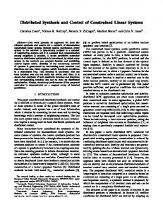
which proves that E (S, ) is invariant under the nonlinear dynamics (1). Theorem 4.1: The spectrogram-MPC problem formulated onto the nonlinear system (1) with terminal constraint xN 2 E (S, ) is recursively feasible. Proof: The proof follows the same lines as in the linear case. As the set E (S, ) is invariant under the nonlinear dynamics, shifting the optimal sequence from the current step and appending the LQR solution u = Kx provides a feasible solution to problem (8) at the next time instant. Satisfaction of the spectrogram constraint computed on the nonlinear dynamics at time N + M is guaranteed by Lemmas 4.1 and 4.2 and the appropriate choice of the terminal constraint formulated in Lemmas 4.3 and 4.4. Theorem 4.2: The closed-loop nonlinear system under the spectrogram-MPC control law is locally asymptotically stable, with basin of attraction equal to the feasible set of the spectrum constrained NMPC problem (8). Proof: Stability of the closed-loop system follows from recursive feasibility and the fact that the terminal cost satisfies the standard decrease Assumption (3.4). V. N UMERICAL E XAMPLE Oscillations are very common in mechanical systems and are responsible, e.g., for fatigue and failure of engines, and thus control techniques for active vibration damping are required [10]. In this section, an example illustrating the efficacy of the proposed spectrum constrained NMPC approach for damping resonance frequencies in constrained nonlinear systems is presented. In practice, many oscillatory dynamical systems can be modelled as linear resonators with a nonlinear restoring force [9]. Therefore, we consider the constrained nonlinear system ◆ ✓ ◆ 8✓ ◆ ✓ 0 x2 x˙ 1 0 > > = + u > > x˙ 2 100 !02 x1 + ✏x21 2⌫!0 x2 > > ✓ ◆ > < x1 z= 1 0 x2 > > > > > |x1 | 15, |x2 | 100 > > : |u| 100 ,
where ✏ = 0.1, !0 = 2⇡ · 12 rad/sec and ⌫ = 2 · 10 4 . System (27) is first controlled to track a piecewise constant reference signal zref = ±0.5 using a standard NMPC formulation without spectrogram constraints. The continuous dynamics
are sampled at 50 Hz and discretised by applying a RungeKutta method of order four. The linearised model around the origin is given by (2) with ✓ ◆ ✓ ◆ 0 1.00 0 AL = , BL = . (27) 5.68 · 103 0.0030 100
The stabilising control law used in the spectrum constrained 0.87 0.14 . The stage cost of NMPC problem is K = (8) is defined as a quadratic function l (x, u) := x> Qx+u> Ru with Q = 100 · I and R = 1. When the system output tracks the upper constant reference +0.5, a resonance can be observed around 12.1 Hz, whereas when tracking the lower reference 0.5, the resonance is obtained around 10.5 Hz, as shown in the time domain trajectory in Fig. 1(a) and the spectrogram in Fig. 2(a). Spectrogram constraints are then incorporated into the NMPC problem. A 3rd order Butterworth filter has been chosen with a window length M = 25, the prediction horizon being N = 30. The spectrogram constraint parameter ↵ is set to 0.1. A constraint is first enforced at 10.5 Hz, which results in the spectrogram in Fig. 2(b). The constraint on the first resonance is then removed and a constraint at 12.1 Hz is added, resulting in the spectrogram in Fig. 2(c). Finally, both resonances are constrained, as shown in the spectrogram of Fig. 2(d). The corresponding closed-loop trajectories are shown in Fig. 1(a), (b), (c) and (d) respectively. The spectrum constrained NMPC strategy proves effective at damping nonlinear resonances. It should be noted that a waterbed effect can be observed in spectrograms (b) and (d), where damping the first resonance seems to amplify the second one, and damping both resonances results in some energy transfer to lower and higher frequencies. VI. C ONCLUSION A novel NMPC scheme for shaping of the harmonic response of constrained nonlinear systems has been presented. The main idea is to enforce hard constraints on the system’s output spectrogram within a receding-horizon optimal control problem. Recursive feasibility of the proposed spectrum constrained NMPC problem, and asymptotic stability of the resulting nonlinear closed-loop system, are enforced by an ellipsoidal terminal constraint. Finally, the effectiveness of the proposed approach has been demonstrated on a small-scale nonlinear resonant system. R EFERENCES [1] B.D.O. Anderson and J.B. Moore. Optimal control, Linear quadratic methods. Prentice-Hall International, 1989. [2] J. Arrillaga and N.R. Watson. Power System Harmonics. Wiley, 2003. [3] P. Cort´es, J. Rodr´ıguez, D.E. Quevedo, and C. Silva. Predictive current control strategy with imposed load current spectrum. IEEE Transactions on Power Electronics, 23(2):612–618, March 2008. [4] R. Gondhalekar, C.N. Jones, T. Besselmann, J.-H. Hours, and M. Mercang¨oz. Constrained spectrum control using MPC. In Proceedings of the IEEE Conference on Decision and Control, pages 1219–1226, Orlando, USA, 2011. [5] J.-H. Hours, M.N. Zeilinger, R. Gondhalekar, and C.N. Jones. Spectrogram-MPC: Enforcing hard constraints on system’s output spectra. In Proceedings of the American Control Conference, pages 2010– 2017, Montreal, CA, 2012. [6] H. Michalska and D.Q. Mayne. Robust receding horizon control of constrained systems. IEEE Transactions on Automatic Control, 38(11):1623–1633, 1993.
6
(a)
(a)
8
1
4
10
z
Hz
3
0
12 2 14 1 16
0
(b)
2
4
6
8
10
1
(b)
1
2
3
4
5
6
7
8
9
8
0
4
10 3
0
Hz
z
12 2 14 1
0
(c)
2
4
6
8
16
10
1
1
(c)
2
3
4
5
6
7
8
9
8
4
10
0
3
Hz
z
0
12 2 14
0
(d)
2
4
6
8
1
10
16
1
1
(d)
2
3
4
5
6
7
8
9
8
z
0
0
4
10
Hz
3 12 2 14 0
2
4
6
8
10
Time (s) Fig. 1. Closed-loop output trajectories: Without spectrum constraint (a), with spectrum constraints at 10.5 Hz (b), with spectrum constraints at 12.1 Hz (c), and with spectrum constraints at both frequencies (d).
[7] A.V. Oppenheim and R.W. Schafer. Discrete-Time Signal Processing. Prentice Hall, 1999. [8] A. Pavlov, N. van de Wouw, and H. Nijmeijer. Frequency response functions for nonlinear convergent systems. IEEE Transactions on Automatic Control, 52(6):1159–1165, 2007. [9] Z.K. Peng, Z.Q. Lang, and S.A. Billings. Resonances and resonant frequencies for a class of nonlinear systems. Journal of Sound and Vibration, 300:993–1014, 2007. [10] A. Preumont. Vibration control of active structures : An introduction. Springer, 2002. [11] D.E. Quevedo, H. B¨olcskei, and G.C. Goodwin. Quantisation of filter bank frame expansions through moving horizon optimisation. IEEE Transactions on Signal Processing, 57(2):503–515, 2009. [12] J.B. Rawlings and D.Q. Mayne. Model Predictive Control: Theory and
1 16 1
2
3
4
5
6
7
8
9
0
Time (s) Fig. 2. Spectrograms of the output signal of the closed-loop system: No spectrum constraint (a), spectrum constraint at 10.5 Hz (b), at 12.1 Hz (c), and at both resonances (d).
Design. Nob Hill Publishing, 2009. [13] A. W¨achter. On the implementation of a primal-dual interior point filter line search algorithm for large-scale nonlinear programming. Mathematical Programming, 106(1):25–57, 2006.