Constrained Subspace Skyline Computation Evangelos Dellis1 Akrivi Vlachou1 Ilya Vladimirskiy1 Bernhard Seeger1 Yannis Theodoridis2 University of Marburg, {dellis, vlachou, ilya, seeger}@mathematik.uni-marburg.de 2 University of Piraeus,
[email protected]
ABSTRACT In this paper we introduce the problem of Constrained Subspace Skyline Queries. This class of queries can be thought of as a generalization of subspace skyline queries using range constraints. Although both constrained skyline queries and subspace skyline queries have been addressed previously, the implications of constrained subspace skyline queries has not been examined so far. Constrained skyline queries are usually more expensive than regular skylines. In case of constrained subspace skyline queries additional performance degradation is caused through the projection. In order to support constrained skylines for arbitrary subspaces, we present approaches exploiting multiple low-dimensional indexes instead of relying on a single highdimensional index. Effective pruning strategies are applied to discard points from dominated regions. An important ingredient of our approach is the workload-adaptive strategy for determining the number of indexes and the assignment of dimensions to the indexes. Extensive performance evaluation shows the superiority of our proposed technique compared to its most related competitors.
Categories and Subject Descriptors H.2.4 [Database Management]: Systems – Query processing
General Terms Algorithms, Design, Performance
Keywords Skyline Queries, High-dimensional Indexing.
1. INTRODUCTION The skyline operator and its computation have attracted much attention recently. This is mainly due to the importance of various skyline results in applications involving multi-criteria decision making. Given a set of d-dimensional objects, the operator returns all objects pi that are not dominated by another object pj. Consider for example a database containing information about cars. Each Permission to make digital or hard copies of all or part of this work for personal or classroom use is granted without fee provided that copies are not made or distributed for profit or commercial advantage and that copies bear this notice and the full citation on the first page. To copy otherwise, or republish, to post on servers or to redistribute to lists, requires prior specific permission and/or a fee. CIKM’06, November 6–11, 2006, Arlington, VA, USA. Copyright 2006 ACM 1-59593-433-2/06/0011…$5.00.
tuple of the database is represented as a point in a data space consisting of numerous dimensions. The x-dimension could represent the price of a car, whereas the y-dimension captures its mileage (shown in Figure 1). According to the dominance definition, a car dominates another car because it is cheaper and has run fewer miles. In practice, a user may only be interested in records within the price range from 3000 to 7000 Euro and with mileage reading between 20K and 100K. The example in Figure 1 shows that the traditional skyline (dashed line) fails to return interesting points. A constrained skyline query returns the most interesting points in the data space defined by the constraints. Each constraint is expressed as a range along a dimension and the conjunction of all constraints forms a hyper-rectangle in the ddimensional data space. 120000 100000
Mileage reading
1
80000 60000 40000 20000 0 0
1000
2000
3000
4000
5000
6000
7000
8000
9000
10000
Price
Figure 1: Constrained skyline in 2-d subspace On the other hand, skyline analysis applications usually provide numerous candidate attributes, and various users may issue queries regarding different subsets of the attributes depending on their interests. While the dimensionality of the corresponding data space might be rather high, skyline queries generally refer to a low dimensional subspace. In our running example, a car database could contain many other attributes of the cars, such as horsepower, age and fuel consumption. A customer that is sensitive on the price and the mileage reading (2-dimensional subspace in Figure 1) would like to pose a skyline query on those attributes, rather than on the whole data space. By combining constrained and subspace skyline queries, we provide a powerful operator that returns the really interesting objects to the user. The constrained subspace skyline queries form the generalization of all meaningful skyline queries over a given dataset. Maintaining a high-dimensional index to support constrained skyline queries in arbitrary dimensionality is generally not suitable. It has been shown that the performance of such highdimensional indexes deteriorates with an increasing number of dimensions [3]. Only low-dimensional indexes, e.g. R-trees, seem
to perform well in practice and for that reason have found their place in commercial database management systems (DBMS) [14]. Especially in applications which involve constrained subspace skyline retrieval a multi-dimensional index over the whole data space shows poor performance. As shown in [18], constrained skyline queries, whose constraint regions cover more than a specific portion of the data space, are usually more expensive than regular skylines. Even a range very close to 100% is much more expensive than a conventional skyline. This effect is even more crucial when subspace skyline queries are applied where additional performance degradation is caused through the projection. In order to employ low-dimensional indexing for constrained subspace skyline queries, we partition vertically the data space among several low-dimensional subspaces and index each of these subspaces using an R-tree. The query is evaluated by merging the partial result from all affected indexes and simultaneously prunes away the dominated data spaces. The benefit of this approach is twofold. Firstly, the low-dimensional queries are processed by low-dimensional and well-performing indexes. Secondly, this approach can easily be adapted to the underlying query workload. The constrained subspace skyline computation over vertically partitioned data has several technical challenges. An algorithm to merge the partial results into the skyline result set is required. An important performance parameter is the pruning strategy. It is desirable to use multiple points to define pruning regions. Finally, the strategy that partitions vertically the data space among several low-dimensional subspaces influences the overall performance. Our contributions can be summarized as follows: •
We address the problem of constrained subspace skyline queries and we present a skyline algorithm (called STA), which exploits multiple indexes.
•
We propose different pruning strategies to identify dominated regions and to discard irrelevant sub-trees of the indexes. We solve effectively the problem of using multiple points for discarding vertically distributed data points during skyline computation.
•
A workload-adaptive strategy for determining the number of indexes and the assignment of dimensions to the indexes is presented.
•
An extensive performance evaluation shows that the new algorithm significantly outperforms existing approaches.
The rest of the paper is organized as follows: The next Section discusses related work. In Section 3 we present our basic STA algorithm and in Section 4 an improved pruning strategy is proposed. In Section 5 we provide an approach for determining the number of indexes and the assignment of dimensions to the indexes. The experimental results are presented in Section 6. Finally, Section 7 concludes the paper.
2. RELATED WORK Skyline computation has recently received considerable attention in the database research community. BNL [4] compares each point of the database with every other point, and reports it as a
result only if it is not dominated by any other point. DC [4] divides the data space into several regions, calculates the skyline in each region, and produces the final skyline from the points in the regional skylines. SFS [6], which is based on the same principle as BNL, improves performance by first sorting the data according to a monotone function. Index-based techniques are proposed in several works. Tan et al. [21] presents the first progressive techniques, namely Bitmap and Index method. Both methods can output the skyline without having to scan the whole dataset. In [15], a skyline computation algorithm based on nearest neighbor search on the indexed dataset is presented. Papadias et al. [17] propose a branch and bound algorithm to progressively output skyline points of a dataset indexed by an R-Tree. One of the most important properties of this technique is that it guarantees the minimum I/O cost for a given R-tree. An extension of their algorithm to deal with constrained skyline queries is also provided. SUBSKY recently proposed in [22] is related to our work as it addresses subspace skyline retrieval. This method transforms the multi-dimensional data into one-dimensional, and therefore permits indexing the dataset with a B-tree. SUBSKY is unable to answer effectively constrained subspace skyline queries as all points have to be transformed in a preprocessing step. Recently, Pei et al. [19] and Yuan et al. [25] independently proposed the Skyline Cube (SKYCUBE), which consists of the skylines in all possible subspaces. The compressed SKYCUBE to deal with frequent updates is proposed in [24]. Even for applications that are restricted to constrained subspace skyline computation, the whole dataset must be indexed. It is not possible to pre-calculate the points of the full space skyline and their duplicates, since the result depends on the given constraints. Finally, there are some other skyline algorithms developed for different purposes. Wu et al. [23] addresses the problem of constrained skyline computation in a distributed P2P environment. Huang et al. in [13] study skyline computation over mobile devices. Balke et al. [1] consider skyline retrieval in distributed environments; Lin et al. [16] investigate continuous skyline monitoring on data streams, and Chan et al. [5] study partially-ordered domains. These approaches differ from the topic of this paper as they are restricted to their specific scenarios. Beyond skyline computation, our work is related to [7], where vertically distributed nearest neighbor queries are examined.
3. CONSTRAINED SUBSPACE SKYLINE COMPUTATION FOR UNIFORM DATA In order to employ low-dimensional indexing for constrained subspace skyline queries, we partition vertically the data space among several low-dimensional subspaces and index each of these subspaces using an R-tree. A constrained subspace skyline query is then partitioned among several sub-queries, each of them is processed by utilizing the corresponding index. We distinguish between two different cases. Firstly, the queried subspace is a subset of one indexed subspace. A modification of a standard index-based constrained skyline algorithm like [18] that additionally simply ignores the irrelevant attributes can be used for the skyline computation. Secondly (the most complicated case), the queried subspace is not entirely covered by any of the
indexed subspaces. In this case, the constrained skyline of a specified subspace is computed by merging the results of constrained nearest neighbor queries that are running simultaneously on some of the low-dimensional indexes in a synchronized fashion. In this section, we present an elegant solution for merging the query results over the involved indexes. To answer constrained skyline queries on an arbitrary subspace, it is necessary that every involved attribute belongs to at least one subspace. We restrict our analysis assuming that every attribute belongs to exactly one subspace. The remaining of this Section is organized as follows: after the problem definition (subsection 3.1), we propose an effective pruning strategy (subsection 3.2) and present our algorithm (subsection 3.3).
3.1 Preliminaries Let S be a data space defined by a set of d dimensions {d1, d2, .., dd} and a domain dom(S). Let D ⊆ dom(S) denote the data set; a point p∈D can be represented as p = {p1, p2, …, pd} where every pi is a value on dimension di. Each non-empty subset S΄ of S (S΄⊆ S) is called a subspace. A point p∈D is said to dominate another point q∈D on subspace S΄ if (1) on every dimension di∈S΄, pi ≤ qi; and (2) on at least one dimension dj∈S΄, pj < qj denoted as p S΄ q. The skyline of a space S΄⊆ S is a set D΄⊆ D of so-called skyline points which are not dominated by any other point of space S΄. That is, D΄ = {p∈D | ¬∃q∈D: q S΄ p}. Based on the definition of skyline points of a subspace, we define the constrained subspace skyline. Let C = {c1, c2, ..., ck} be a set of range constraints on subspace S΄ = {d1΄, d2΄, ..., dk΄} where k ≤ d. Each ci is expressed by [ci,min, ci,max], where ci,min ≤ ci,max, representing the minimum and maximum value of di΄. A constrained skyline of a space S΄ ⊆ S refers to the set of points Dc΄ = {p∈Dc| ¬∃q∈Dc: q S΄ p}, where Dc ⊆ D and Dc = {p∈D | ∀di∈ S΄: ci,min ≤ pi ≤ ci,max}. For a point p∈Dc of the subspace S΄, the dominance region DRS΄,C(p) is {q∈dom(S’)c | p S΄ q}. Similarly, the antidominance region ADRS΄,C(p) of a point p refers to the set of points dominating p. In Figure 2, the dominance and antidominance regions of a point are illustrated. A straightforward observation is that a point q falls within the dominance region of p, if and only if p falls within the anti-dominance region of q. DR of p
c2,max
d2
Constrained Region
p c2,min
c1,max
Proof. (sketch) Let point p∈Dc be a skyline point in S΄ and let us assume to the contrary that there exists a point q which belongs to ADRSi’,C(p) for each subspace Si΄, 1 ≤ i ≤ n. Since ∀dj∈ Si΄, pj < qj (1 ≤ i ≤ n) and ∪ Si΄ = S΄, it follows ∀di ∈ S΄, pi < qi . Thus, q is dominated by p in S΄ and it is not in ADRSi’,C(p), which contradicts our assumption. ■ Lemma 1 gives us a powerful rule to determine whether a point p is dominated by a point q or not. Note that p is not dominated by q if and only if p’s projection is not dominated by q’s projection in at least one Si΄. If the dominance test returns true in all subspaces, we immediately obtain that q dominates p. In the case where the distinct value condition does not hold, all objects that are equal to p in one of the n subspaces Si΄ have to be examined.
3.2 Pruning with the Nearest Neighbor In this subsection we propose a pruning strategy using only one point for pruning. Based on Lemma 1, we can discard all points that fall in the dominance area of a point in every subspace Si΄ without losing any skyline point. Any point may be used for pruning, but it is desirable that the chosen point prunes in all subspaces Si΄ equally well and maximizes the total number of discarded points. Moreover, the point should be computed fast in order to apply pruning very early. In our one-point pruning strategy, we suggest using the nearest neighbor with respect to the Manhattan distance to the lower left corner of the constrained region of subspace S΄. The reasons for choosing this point are as follows. Firstly, because it is a member of the skyline, there is no dominating point. Secondly, among all the skyline points it is the one with maximum perimeter of the dominance region. Because perimeter and volume are highly correlated, this also gives a large volume on average, and hence, it is also expected to prune a large percentage of the data points. In the following, we present the results of an empirical analysis of the size of the dominance region assuming N data points being independently and uniformly distributed in the d-dimensional unit cube. In Figure 3, the expected value of the volume is plotted as a function of the dimension. As illustrated, we obtain large regions for low- and medium-dimensional data, while the pruning effect deteriorates with an increasing dimensionality. Moreover, we have observed that the volume of the pruning area of the selected point is only slightly smaller than the maximum volume of a point. 1
ADR of p
c1,min
Lemma 1. A point p∈Dc is a skyline point in S΄ if and only if there exists no point q∈Dc that belongs to the anti-dominance area of p for all subspaces Si΄ (1≤ i ≤ n).
d1
0,9 0,8 0,7 0,6
Figure 2: Dominance region of p Let us assume that the subspace S΄ is vertically distributed over n subspaces Si΄ (∪Si΄ = S΄, 1 ≤ i ≤ n). Every Si΄ has an associated constraint Ci (∪Ci = C, 1 ≤ i ≤ n). In the following, we present a lemma that allows us to identify skyline points using only the subspaces. We first assume that the distinct value condition holds [19], [25]. Later, we relax this assumption.
0,5 0,4 0,3 0,2 0,1 0 0
1 2
3
4 5
6
7 8
9 10 11 12 13 14 15 16 17 18 19 20
Dimensionality
Figure 3: Volume of the pruned area
3.3 STA: A Threshold-based Skyline Algorithm Let us assume that the data space consists of the subspace S, while each of the n indexes Ri corresponds to a subspace Si (1≤ i ≤ n). A constrained skyline query refers to a subspace S΄ under constraint C. The skyline query is partitioned into n sub-queries, each of which refers to a subspace Si΄ (∪Si΄ = S΄) under constraint Ci (∪Ci =C). The points are retrieved through incremental constrained nearest neighbor search on each index i based on the distance to the lower left corner of the constrained region according to the subspace Si΄. The retrieved points are merged into a skyline result set. Notice that the dimensionality of the indexed subspace Si and that of the queried dimension subset Si΄ are not necessarily equal. Thus, during the nearest neighbor search, irrelevant dimensions are ignored. Moreover, the points are delivered in order of their Manhattan distance to the lower left corner of the constrained region according to subspace Si΄. We first assume that the distinct value condition holds [19], [25]. Later, we relax this assumption. Our algorithm consists of two steps: a filter step and a refinement step. In the filter step, the points in each subspace Si΄ are accessed simultaneously based on the sorting according to subspace Si΄. Points outside the constrained region are immediately discarded. In the refinement step, a potential skyline point, also called a candidate, is tested for domination. The refinement step needs to determine whether this candidate is a skyline point or not. This requires a domination test based on the query subspace S΄. Because each index Ri return the points in a strictly monotonic order, a point p retrieved from Ri could only be dominated by points that are retrieved from Ri before p. Thus, we need to test a point for domination only with the skyline points that have been already found and we can immediately return a point that is not dominated as a skyline point. The dominance test can be performed in a way similar to traditional window queries [18] using a main-memory R-tree whose dimensionality is equal to the query dimensionality. ALGORITHM 1 outlines our algorithm. The domination test is executed in line 8 by the dominated(Dc΄,S΄) function which tests if the candidate is dominated in S΄ by any already founded skyline point. While the n indexes Ri are accessed simultaneously, our algorithm targets to find quickly the first constrained nearest neighbor in S΄. Thus, we keep the point with the smallest distance as a potential nearest neighbor and we use the Manhattan distance of the last reported point of Si΄ as a threshold to find the nearest neighbor. This leads to an algorithm which is similar to Fagin’s TA threshold algorithm [8] for list merging. As soon as the constrained nearest neighbor according to S΄ is found, we can discard all points that belong to the dominance area of the nearest neighbor in each subspace Si΄ (due to Lemma 1). In fact, the incremental constrained nearest neighbor search is executed with respect to a pruning area. During the incremental constrained nearest neighbor search internal and leaf nodes are discarded if they are entirely covered by the pruning area. In ALGORITHM 1 the nextNN function (line 6) returns the constrained nearest neighbor with respect to a pruning area. The pruning area is set when the first nearest neighbor is found (lines 13-16). An index scheduler determines the order in which the indexes are visited. A naive way for visiting the indexes is a round robin strategy. This however ignores the fact that we strive for fast
computation of the nearest neighbor, and that the indexes differ in their performance. Therefore, we are interested in more advanced strategies resulting in a fast increase of the threshold. The underlying assumption of our advanced scheduling strategy of the indexes is that an index that has been productive in the past will continue to be in the near future. Therefore, we advance the processing with the index that will maximize the benefit for increasing the threshold. ALGORITHM 1: STA(Subspace S’, Constraints C) 1: Dc΄ = {}; // the constrained subspace skyline set 2: d = maxDistance; // d represents the distance to the current NN 3: pruning_area = null; //the pruning area 4: ind = index_scheduler(); 5: while (1 ≤ ind ≤ n) do 6: o = Rind.nextNN(Sind’,Cind); //returns the next local NN in Sind 7: dind = distance(o, Sind’,Cind); 8: if ((o ∈ Dc)&&(not o.dominated(Dc΄,S΄)) then 9: Dc΄.insert (o); 10: if ((distance(o, S’,C) < d )&&(pruning_area == null)) then 11: nn_Candidate = o; 12: d = distance(nn_Candidate, S’,C); 13: if (d < d1+...+dd )&&(pruning_area == null)) then 14: pruning_area = DRS΄,C(nn_Candidate); 15: for (1 ≤ i ≤ n) do 16: Ri.pruning_area= DRSi΄,Ci(nn_Candidate); 17: ind = index_scheduler(); 18: return Dc΄;
ALGORITHM 1 abstracts from some of the implementation details related to the organization of the multidimensional points. The naïve approach is to keep in each of the low-dimensional indexes the entire points. However, this causes a high storage overhead. A more advanced approach is to store only the associated attributes of the subspaces in the index and to keep a copy of the entire point in a hash-table where the point can be retrieved using its associated identifier. Each time a point is received from one of the indexes, the entire record information is read from the hash-table. In case where the distinct value condition does not hold, a point may be added to the result set Dc only if all points with the same distance in Si΄ are examined.
4. IMPROVED PRUNING FOR ARBITRARY DISTRIBUTIONS The main disadvantage of the previous pruning strategy is that only one point is used for pruning. In the previous section, we showed that the nearest neighbor is expected to prune a high percentage of a uniformly distributed dataset, but for real datasets, the pruning power of the nearest neighbor may diminish. In this section we propose a pruning strategy that allows us to enlarge the dominance area using multiple points for pruning.
4.1 Motivating Example We begin with the following motivating example to show the limited applicability of the nearest neighbor pruning strategy. Let
us consider a non-uniform dataset consisting of clusters as it is illustrated in Figure 4 where two clusters exist.
d2 d4
p3
p1
As illustrated, only roughly half of the points belong to the dominance area of the first nearest neighbor. As a consequence, all remaining points need to be retrieved and tested for domination. y
DRy(p2)
DRy(p1)
p1 p2 O
x DRx(p1)
p1
p2 d1
d3
Figure 5: Pruning strategy Unfortunately, by following this strategy some skyline points can still be falsely discarded. In Figure 6, we give an example. Let the point q in the subspace S2 collapse on the point q1. The point p, based on Lemma 1, is not a skyline point in S, since it is dominated by q in all dimensions sets of S. On the other hand, if the point q in the subspace S2 collapses on the point q2, then point p may be discarded falsely, since it is a potential skyline point.
DRx(p2)
d2 d4
Figure 4: Simultaneous pruning Our goal is therefore to prune the data space using multiple points. Let us first consider a straightforward generalization of the algorithm presented in Section 3.3. Considering Figure 4 after retrieving the first nearest neighbor p1, the pruning area in both projections DRx(p1) and DRy(p1) is discarded and we continue expanding the local indexes until we find the second nearest neighbor p2 (assuming that it is not dominated by the first nearest neighbor). When trying to prune in both projected subspaces with the second nearest neighbor, we may falsely discard skyline points located in the left-lower rectangle. While it seems to be easy to determine the region where skyline points may be falsely discarded, this region enlarges and is difficult to define for a higher query dimensionality and a larger number of subspaces. As a consequence, we are not able to prune simultaneously in both subspaces using the same point. To overcome this problem, we make the following observation: when points lying in the dominance region of a point are not discarded in at least one subspace, then we are able, under certain conditions, to discard points in all remaining subspaces, while we still guarantee no false dismissals. Therefore, we use the points that are retrieved as local constrained nearest neighbors from an index for pruning in all other indexes. Local nearest neighbor points outside the constrained region in the query space are discarded and not used for pruning. In contrast to the nearest neighbor strategy of Section 3.2, this new pruning strategy also provides the advantage of discarding points already before the first nearest neighbor is found. For sake of simplicity, we assume in the rest of this section that there are no constraints, i.e., the skyline query refers on the whole dataset. It is straightforward to adapt the strategy to constrained subspace skyline queries by ignoring the irrelevant dimensions and discarding points that do not belong to the Dc. Let us now consider the example in Figure 5, where a 4dimensional data space is divided into two 2-dimensional subspaces. When the point p1 is retrieved from subspace S1 then the dominance area of the point p1 in subspace S2 is used for pruning.
p
p2
p
q2 q
p1
q1 d1
p3 d3
Figure 6: Example of Pruning Strategy In the next subsection we investigate this case in more detail by providing a lemma which helps us to ensure that we do not discard points falsely.
4.2 Improved Pruning using Multiple Points We now present a pruning strategy that ensures that the entire skyline set is returned and no point is falsely discarded. Let us continue with our running example with two 2-dimensional subspaces. Each time a new point is retrieved from subspace S1 this point is a candidate for pruning in subspace S2. Let us first introduce an important notation. The discarded region dis(Si) of a subspace Si consists of points p such that all points in the dominance region of p can be discarded. For example in Figure 6, the discarded area of S2 is dis(S2)= {p2, p3}. Let us now assume that the discarded region of S1 consists of the points p1, p2, …, pm. To discard points from the dominance area of p in S2, the point p and a point pi must be dominated in both subspaces by the same point, called a common point,. This condition must hold for each point pi which belongs to the discarded area of S1. Since the complexity of this test is high, and in order to keep the overhead low, we restrict the search for a common point to the following two conditions (assuming n=2): •
The projection of point pi belongs to the anti-dominance area of p in S2, or
•
The projection of point p belongs to the anti-dominance area of pi in S1.
If one of the two conditions holds for each point pi the dominance area of the projection of point p in S2 can be discarded. In Lemma 2, we generalize these conditions for arbitrary n.
d2 d4
p1 p1 d1
d3
d2
p2
d4
q
p1
p1
q
p2
1400
d1
d3
1000
p3
d4
p2
p1 p3
p1
p2
One Point
800 600 400 200
d1
Subspace S1
Multiple Points
1200 Page Accesses
d2
In order to confirm the accuracy of the multiple points pruning strategy, we study the performance of our STA algorithm using real world datasets (cnf. Section 6). We examine constrained subspace skyline queries of lower dimensionality. Each workload contains 100 queries that request the skylines of 100 random subspaces with fixed dimensionality dsub=3. We set the constrained region to cover 60% of each (queried) axis. We report the number of page accesses required for calculating the skyline.
d3
Subspace S2
Figure 7: Improved pruning heuristic We illustrate these conditions by an example depicted in Figure 7. Again, the data space S is divided into two subspaces, S1 and S2. The left column contains projections of points in subspace S1, whereas the right column contains projected points in S2. Points are retrieved using local nearest neighbor search. The point p1 is found in subspace S1. Since no point is used for pruning the dominance area of p1 in subspace S2 can be discarded. In the second step (assuming round-robin retrieval), the point p2 in subspace S2 is retrieved. The anti-dominance area of p1 in subspace S2 contains point p2 which means that p2 dominates p1 in S2. It is not possible that a point that belongs to both dominated regions, for example point q, to be a skyline point since it is dominated by p1 and p2 in S. After this, by retrieving the next point p3 in subspace S1, the antidominance area of p2 does not contain p3 in S1, but the antidominance area of p3 contains point p2 in subspace S2. This guarantees that a point which is pruned by both discarded areas is dominated based on Lemma 1. The following Lemma is necessary to generalize the previous strategy for n subspaces. Lemma 2. Let u(Si) be the projection of point u in subspace Si. No point is falsely discarded, if for each tuple (u1(S1), u2(S2), ..., un(Sn)) ∈ dis(S1) x dis(S2)x … x dis(Sn) there exists a k (1 ≤ k ≤ n) such that ∀ i ≠ k uk(Si)∈ADRSi(ui(Si)). Proof. (sketch) Let p be a skyline point that is discarded by the pruning strategy, then p must be discarded in all subspaces Si. Thus, for every Si there exists a point ui(Si)∈dis(Si) for which p∈ADRSi(ui(Si). Since for each tuple of dis(S1)xdis(S2)x… x dis(Sn) there exists a k (1 ≤ k ≤ n ) such that ∀ i ≠ k uk(Si)∈ADRSi(ui(Si)), based on Lemma 1 the point p is dominated in S by the point uk and is not a skyline point. This leads us to a contradiction. ■ Generalizing the previous strategy, each time a point p should be added to the discarded area of Sk, the condition must hold for all tuples (u1(S1),…,uk-1(Sk-1), p, uk+1(Sk+1),… un(Sn)). For the efficient implementation of the pruning mechanism, n main memory Rtrees are used, each of them with a dimensionality of the corresponding Si, and keeping the points that participate to the discarded area of Si. While the visited points according to the partial sorting imply the region our algorithm examines, these main-memory indexes implement the discarded region.
0 9
13 Dataset Dimensionality
32
Figure 8: Pruning Strategies Figure 8 reports the effect of the different pruning strategies. As expected, the improved pruning strategy using multiple points for pruning is superior to the strategy which uses only one point for pruning except for the 13-dimensional dataset. However, the onepoint pruning strategy works very well even for real datasets. Finally we adapt our scheduler for the case of the improved pruning strategy. In the case of the nearest neighbor pruning strategy, it is important to speed up the merging phase and find quickly the first nearest neighbor. In the improved pruning strategy it is more important to prune equally large regions over all indexes. When an index delivers the next point, this point may be used for pruning in all indexes except the index that delivered this point. In the case where an index has a high number of pruning points, while another index has only few, the first index performs very well, in contrast to the other that will perform very poorly. Thus, we give the control to this index that has the most pruning points, so that the other indexes have the opportunity to enlarge their discarded regions.
5. ADAPTIVE SUBSPACE INDEXING USING LOW-DIMENSIONAL R-TREES In this section we present an algorithm to distribute the data space over multiple indexes. This method is very effective, especially in applications which involve constrained subspace skyline retrieval, where a multi-dimensional index over the whole data space shows poor performance. As shown in [18], constrained skyline queries, whose constraint regions cover more than a specific portion of the data space, are usually more expensive than regular skylines. This effect is even more crucial when subspace skyline queries are applied. In case of subspace skyline queries additional performance degradation is caused through the random grouping effect (which is explained later in this section). Even for applications that are restricted to constrained subspace skyline computation, the whole dataset must be indexed. It is not possible to pre-calculate the points of the full space skyline and their duplicates, since the result depends on the given constraints. In the following section we provide a formula for determining an appropriate number of indexes (subsection 5.1). A greedy algorithm which assigns the attributes to the indexes is developed
5.1 Number of Indexes In this section we present a formula for determining the number of indexes. Toward this goal, we investigate the random grouping effect of a multidimensional index. Our goal is to make clear why a high-dimensional index is not appropriate for subspace skyline computation and how low-dimensional indexes can avoid performance degradation. The performance of low-dimensional constrained skyline queries decreases when the dimensionality of the indexed space becomes high while the dimensionality of the query space remains low. This is mostly caused by the random grouping effect. Since not all dimensions are used as split axis for splitting a leaf node during the index creation. When a query that requires projection is posed to the index, the performance of the index is then similar to a random low-dimensional index, i.e., an index that groups the points into leaf nodes in an almost random manner. As an example consider a 10-dimensional data space and assume that we are interested in retrieving the skyline of any 2-dimensional subspace. If only two of the dimensions are used for splitting, then the probability that the query dimensions have been used for splitting is very small. Thus, the query performance is similar to the performance of a 2-dimensional index, where the data points were grouped together randomly. We are now modeling this effect in a more formal way. We assume uniformity and independence in the data distribution. If every leaf node is split at least once in each dimension, we need a total number of at least 2d leaf nodes. Given the effective data page capacity Ceff of the R-tree, which depends on the index dimensionality, the number of leaf nodes can be estimated as:
⎡ N ⎤ L=⎢ ⎥ ⎢ C eff ⎥ . We define an index as well performing if L ≥ 2d, which means that every leaf node is split by each dimension once. The maximum dimensionality for which a low-dimensional index fulfils the above property is:
d max
L = arg min ( 1 − i ) 2 . 1≤i ≤ d
The resulting formula for the number of indexes is: ⎡ d ⎤ n=⎢ ⎥ ⎢ d max ⎥ .
In order to illustrate how to determine the number of indexes, we apply the above formula to the 32-dimensional Color histogram dataset (cfg. Section 6), which consists of 68,040 records corresponding to photo images. In Figure 9, we plot for different values of d the expected random grouping effect, expressed through the formula abs(1-L/2d). Assuming a page size of 4K, the maximum dimensionality dmax for which a low-dimensional index is well-performing for this dataset is 11.
70
N=68,040 Points 60
Random Grouping Effect
to determine the most beneficial subspaces for skyline calculation (subsection 5.2). Finally, we extend our approach to adapt to the query workload (subsection 5.3).
50 40 30 20 10 0 0
1
2
3
4
5
6
7
8
9
10
11
12
Index Dimensionality
Figure 9: Random Grouping Effect Our formula suggests that we should create 3 indexes for this dataset. In this way we index more effectively high dimensional datasets, by avoiding performance degradation due to random grouping effect. After we have shown how to determine the number of indexes, we provide an algorithm to distribute the attributes to the indexes in the next section.
5.2 Attribute Assignment Algorithm In order to build well performing indexes for answering constrained subspace skyline queries, it is of utmost importance to provide effective strategies for distributing the attributes over the n indexes, where n corresponds to the number of indexes defined in the previous section. The strategy is based on a simple cost model that employs the number of distinct values on the performance of STA. During the threshold based skyline calculation, each lowdimensional index returns local skyline points that might be included in the final result set. Independent from the pruning strategy it is impossible to prune the local skyline points, and therefore these points have to be examined in the querydimensional space. There are two different reasons why a point might be later discarded. First, there may be many points whose projections coincide to a low-dimensional point, so that it is dominated by some duplicate point in the query-dimensional space. Second, in the case of constrained subspace skyline queries, a skyline point might be discarded because it is outside of the constrained region in the query-dimensional space. Since the test of discarding points caused by the constrained region has a low computational cost, we focus on the first case. A domination test for all those points is required in a refinement step, even though it is very possible that only few of them are in the skyline of the query-dimensional space. This effect is largely influenced by the number of distinct values in the subspaces. Thus, we propose the number of distinct values dvSi as a quality measure of a subspace Si. Methods to estimate the distinct values can be found in [11]. We propose a greedy algorithm that targets to restrict the random grouping effect, while maximizing the number of distinct values. Let n be the estimated number of indexes. Our greedy algorithm performs as follows: Given n initially empty subspaces Si and a set of unassigned dimensions, the subspace with the smallest distinct values is selected for receiving the next unassigned dimension that maximizes the number of distinct values. This step is repeated until all dimensions are assigned to subspaces.
ALGORITHM 2: assignDimensions(int n, int dmax)
1: D={d1,…,dd}; // precondition: n*dmax ≥ d 2: S ={S1,…,Sn}; // initially: Si =∅, i ≤ i ≤ n 3: while (D is not empty) do 4: Smin = argmin Si∈S {dvSi | |Si| < dmax}; 5: next_dim = argmax d∈D {dvSmin ∪ {d}}; 6: Smin = Smin ∪ {next_dim}; 7: D = D – {next_dim}; 8: return S;
So far, our greedy algorithm tries to choose the subspaces which are more beneficial for a threshold-based skyline algorithm, by minimizing the points that have to be examined. In the next subsection we extend the greedy algorithm to consider the query workload, i.e. how frequent dimensions occur in queries.
5.3 Workload-adaptive Extension The subspaces are unlikely to have the same probability of being requested in a query. Rather, we might be able to associate some probability with each subspace, representing the frequency with which it is queried. The fact that user preferences are highly biased strengthens our approach. Note that it is even more important in such a case to use multiple indexes, which are built on the most preferred subspaces and as a result to guarantee an overall low query response time. A simple, but very powerful extension over our basic model is to weight the cost estimation of each subspace by its frequency. This is a natural way to express the fact that a subspace influences the query performance only if it is requested. This query-adaptive method for creating indexes is very important for supporting the most common queries efficiently. This extension also allows us to examine the performance of our algorithms under a real workload.
6. PERFORMANCE EVALUATION In this section we experientially confirm that our algorithm is both scalable and superior to other techniques. For the experimental evaluation of our approach, three popular data sets are used. Specifically, NBA dataset contains 17,000 13dimensional points, where each point corresponds to the statistics of a player in 13 categories. Color moments contains 9dimensional features of 68,040 photo images extracted from the Corel Draw database. Color histogram consists of 32-dimensional features, representing the histogram of an image. Additionally, we
generated 10-dimensional cardinality.
uniform
datasets
with
varied
In the first set of experiments we study the efficiency of the proposed algorithm on constrained subspace skyline computation. In the second set of experiments, we examine the influence of the dimensionality of the dataset to our algorithm and study the scalability. In a final set of experiments, we investigate the special case in which we request the constrained skyline of a subspace based on a more realistic query workload (in particular, the queries follow the “80-20” rule). In terms of implementation, we set the page size for each R-tree to 4K while each dimension is represented by a real number. Note that we keep the entire points with all their dimensions in each low-dimensional index. In our experimental evaluation mainly we use as a quality measurement the number of I/O. The CPU performance leads to similar results following the same trend.
6.1 Examination of Constrained Subspace Skylines In this section we compare our technique with BBS algorithm [18] which is the best known method for R-tree based skyline retrieval. We index each dataset through a full-space R-tree and a modification of the BBS algorithm that simply ignores the irrelevant attributes is used for constrained subspace skyline computation. We used all real and synthetic datasets, namely NBA, Color moments, Color histogram and Uniform datasets for the following experiments.
6.1.1 Effect of Constrained Region We now study the effect of the constrained region. More particularly we vary the constrained region from 50% to 100% of each dimension. We examine subspaces with dimensionality of 3. For the purpose of this experiment we use the uniform dataset which has a full space dimensionality of 10-d and a cardinality of 50,000 points. 1600
STA
BBS
60
70
1400 1200
Page Accesses
In an initialization step, the number of distinct values for each dimension is separately calculated and the n dimensions with the highest distinct values are assigned to the n subspaces Si. In the next step, we pick the subspace Sh with the minimum number of distinct values. Thereafter, the cost is computed for each remaining dimension di merged with the selected subspace. The dimension contributing to the subspace with the highest distinct values is chosen. By applying the above methodology iteratively, every dimension is assigned to a subspace. This greedy algorithm additionally takes into account that the dimensionality of a subspace is at most dmax. The reason for this limitation is to restrict the random grouping effect. By introducing the threshold dmax, our assignment algorithm strives to find a balance between the number of the indexes and the dimensionality of each index. As soon as the algorithm terminates, an index is created on each of the subspaces. Our algorithm is illustrated in ALGORITHM 2.
1000 800 600 400 200 0 50
80
90
100
Constrained Region (% of each axis)
Figure 10: Uniform dataset In Figure 10, the x-axis represents the constrained region whereas the y-axis measures the page accesses required to compute the subspace skyline within the constrained region. We compare our STA algorithm against BBS. Our algorithm is consistently superior. Note that, a range close to 100% is much more expensive than a conventional subspace skyline. However, for constrained subspace skyline queries our algorithm is generally more effective requiring less page accesses than BBS for arbitrary large constrained regions. A crucial observation is that the performance of our algorithm is not affected significantly by the size of the constrained region.
In this section we compare our algorithm with BBS on constrained subspace skyline computation with respect to the subspace dimensionality. For the first experiment of this section we used the 10-dimensional Uniform dataset which has a cardinality of 50,000 whereas for the second experiment we used the 9-dimensional Color moments dataset. We compare our STA algorithm with BBS, again by varying the query subspace dimensionality from 2 to 4. 1200
Page Accesses
Page Accesses
STA
1000 800 600 400 200
800 600 400 200
3
4
0 2
Subspace Dimensionality
3
Subspace Dimensionality
4
Figure 11 : Uniform and Color Datasets The left part of Figure 11 captures the performance of STA and BBS by reporting the measured page accesses for different subspaces with varied dimensionality for the Uniform dataset. Our algorithm outperforms BBS for this dataset. The right part of Figure 11 reports the number of page accesses for different subspaces with varied dimensionality for the Color moment dataset and using as a query workload random subspaces of fixed dimensionality, namely 2, 3 and 4. These results demonstrate that the STA algorithm leads to substantially less page accesses than BBS.
6.2 Scalability with the Dataset Cardinality and Full-space Dimensionality In order to study the effect of cardinality we use uniform datasets, which have a dimensionality of 10-D, and vary the cardinality between 10,000 and 100,000 points. In addition we request the skyline of 3-dimensional subspaces. Figure 12 shows the number of node accesses with respect to the dimensionality for the Uniform dataset.
Page Accesses
3000
STA
BBS
2500
STA BBS
1400 1200 1000 800 600 400 200
20
0
30
Dataset Dimensionality
9
13
Dataset Dimensionality
32
The chart in Figure 13 compares the I/O performance of STA and BBS in terms of page accesses by varying the full space dimensionality for the Uniform dataset. It is clear that BBS requires more I/Os than STA. The degradation of BBS is mainly due to the poor performance of R-trees in high dimensions and the random grouping effect. Our technique avoids these shortcomings by using indexes of lower dimensionality. Note that these factors also influence STA, but their effect is limited compared to the inherent deficiencies of the BBS algorithm. On the right side of Figure 13, we report the performance of the STA algorithm relative to BBS for the all real datasets. The chart shows that our algorithm is consistently superior. Our algorithm constantly outperforms BBS in both experiments.
6.3 Adaptation to the Query Workload In this section we examine the performance of our algorithm for a query workload which comes closer to real applications. More specifically, we used the “80-20” rule to generate the queries. This means that 20% of the attributes contribute to 80% of the queries, while the remaining 80% of the attributes occurred only in 20% of the queries. The purpose of this experiment is to illustrate the impact of the query workload following the “80-20” rule, on our STA algorithm. 12000
1200 STA
10000
BBS
1000
STA
BBS
8000
800
6000
600
4000
400
2000
200
2000
0 0
1500
2
3
4
Subspace dimensionality
1000 500
2
3
4
Subspace dimensionality
Figure 14: Uniform Dataset
0 10000
1600
Figure 13: Uniform and Real Datasets
0 2
BBS
BBS
1000
1200
STA
C P U T im e (m s e c )
BBS
1400
4500 4000 3500 3000 2500 2000 1500 1000 500 0
10
Page accesses
STA
1600
To examine the influence of the full-space dimensionality we use the Uniform datasets. Each dataset consists of 50,000 points with a varied full space dimensionality of 10, 20 and 30 respectively. We set the subspace dimensionality constant, namely dsub=3.
Page Accesses
6.1.2 Effect of Subspace Dimensionality
6.2.1 Effect of Full-space Dimensionality
Page A ccesses
From now on, the size of the constrained region is set for each dimension of a query to 60% and 80% for the uniform and the real datasets, respectively.
40000
70000
Dataset Cardinality
100000
Figure 12: Uniform dataset STA clearly outperforms BBS. The performance difference actually increases with an increasing cardinality of the dataset. Hence, the proposed method scales better than BBS.
Figure 14 shows two plots where the left one illustrates the performance of the algorithms in terms of page accesses. The right plot captures the CPU overhead. In both cases, our algorithm constantly outperforms BBS in this experiment. The results confirm that our strategy indeed leads to the best performance, as it adapts to the query workload.
3000
STA
[6] Chomicki, J., Godfrey, P., Gryz, J., Liang, D. Skyline with Pre-sorting. ICDE, 717-719, Bangalore, India, 2003.
BBS
2500
[7] Dellis, E., Seeger, B., Vlachou, A. Nearest Neighbor Search on Vertically Partitioned High-Dimensional Data. DaWaK, Copenhagen, Denmark, August 26-29, 2005
Page Accesses
2000 1500 1000 500 0 10000
30000
50000
70000
Dataset Cardinality
90000
Figure 15: Scalability Figure 15 shows the page accesses for the Uniform dataset as a function of its size. For the case of non-random queries, the performance difference among the methods increases more rapidly with the size of the dataset than it was observed for random queries.
7. CONCLUSION In this paper, we proposed a threshold-based skyline algorithm STA, which efficiently supports constrained skyline queries in arbitrary subspaces by exploiting multiple low-dimensional indexes instead of relying on a single high-dimensional. This avoids the well known deficiencies of indexing high-dimensional data, while available and efficient low-dimensional indexing techniques of general purpose can be employed. The burden of creating these indexes is not left to the user, but we proposed strategies for determining the number of indexes and for assigning the dimensions to the indexed subspaces. The latter strategy does not rely on the data solely, but also takes the query load into account. A threshold-based algorithm supports an efficient merge of the results received from the different indexes, while new pruning strategies were developed for identifying irrelevant points. As shown in our performance evaluation, STA is a very robust and efficient technique for computing constrained subspace skylines even when the dimensionality of the dataset is high. We believe that the problem of supporting constrained subspace skylines is actually more relevant in practical applications as most of the previously considered variants of skylines. STA is the first method particularly designed for processing such queries. Its flexibility and efficiency makes STA very appealing for realworld applications.
8. REFERENCES [1] Balke, W., Gunzer, U., Zheng, J. Efficient Distributed Skylining for Web Information Systems. EDBT, 256-273, Heraklio, Greece, March 14-18, 2004. [2] Beckmann, N., Kriegel, H-P., Schneider, R., Seeger, B. The R*-tree: An Efficient and Robust Access Method for Points and Rectangles. ACM SIGMOD, pages 322-331, 1990. [3] Berchtold, S., Keim, D., And Kriegel, H-P. The X-tree: An index structure for high dimensional data. VLDB, 1996.
[8] Fagin, R., Lotem, A., Naor, M. Optimal Aggregation Algorithms for Middleware. ACM PODS, 102 - 113, Santa Barbara, CA, May 21-23, 2001. [9] Ferhatosmanoglu, H., Stanoi, I., Agrawal, D., Abbadi, A. Constrained nearest neighbor queries. SSTD 2001. [10] Guttman, A. R-Trees: A Dynamic Index Structure for Spatial Searching. ACM SIGMOD, 47-57, Boston, MA, 1984. [11] Haas, P., Naughton, J., Seshadri, S., Stokes, L. SamplingBased Estimation of the Number of Distinct Values of an Attribute. VLDB, pages 311-320, 1995 [12] Hjaltason, G., Samet, H.: Distance Browsing in Spatial Databases. ACM TODS 24(2): 265-318 (1999) [13] Huang, Z., Jensen, C., Lu, H., Ooi, B-C. Skyline Queries against Mobile Lightweight Devices in MANETs. ICDE, 66, Atlanta, Georgia, USA, April 3-7, 2006. [14] Kanth, R., Ravada, S., Sharma, J., Banerjee, J.: Indexing Medium-dimensionality Data in Oracle. SIGMOD 1999. [15] Kossmann, D., Ramsak, F., Rost, S. Shooting Stars in the Sky: an Online Algorithm for Skyline Queries. VLDB, 275286, Hong Kong, China, 20-23 August, 2002. [16] Lin, X., Yuan, Y., Wang, W., Lu, H.: Stabbing the Sky: Efficient Skyline Computation over Sliding Windows. . ICDE, 502-513, Tokyo, Japan, April 5-8, 2005. [17] Papadias, D., Tao, Y., Fu, G., Seeger, B. An Optimal and Progressive Algorithm for Skyline Queries. ACM SIGMOD, 443-454, San Diego, CA, June 9-12, 2003. [18] Papadias, D., Tao, Y., Fu, G., Seeger, B. Progressive Skyline Computation in Database Systems. ACM Transactions on Database Systems, 30(1): 41-82, 2005. [19] Pei, J. Jin, W, Ester, M., Tao, Y.: Catching the Best Views of Skyline: A Semantic Approach Based on Decisive Subspaces. VLDB, pages 253-264, 2005. [20] Roussopoulos, N., Kelly, S., Vincent, F. Nearest Neighbor Queries. ACM SIGMOD, 71-79, San Jose, CA, 1995. [21] Tan, K., Eng, P. Ooi, B. Efficient Progressive Skyline Computation. VLDB, 301-310, Rome, Italy, 2001. [22] Tao, Y., Xiao, X., Pei, J. SUBSKY: Efficient Computation of Skylines in Subspaces. ICDE, Georgia, USA, 2006. [23] Wu, P., Zhang, C., Feng, Y., Agrawal, D., Abbadi, A.: Parallelizing Skyline Queries for Scalable Distribution. EDBT, 112-130, Munich, Germany, March 26-31, 2006.
[4] Borzsonyi, S, Kossmann, D., Stocker, K. The Skyline Operator. IEEE ICDE, 421-430, Heidelberg, Germany, 2001.
[24] Xia, T., and Zhang, D.: Refreshing the Sky: The Compressed Skycube with Efficient Support for Frequent Updates, In Proceedings of 25th SIGMOD, Chicago, IL, 2006.
[5] Chan, C., Eng, P-K., Tan, K-L.: Efficient Processing of Skyline Queries with Partially-Ordered Domains. ICDE, 190-191, Tokyo, Japan, April 5-8, 2005.
[25] Yuan, Y., Lin, X., Liu, Q., Wang, W., Yu, J., Zhang, Q.: Efficient Computation of the Skyline Cube. VLDB, 241-252, Trondheim, Norway, August 30 - September 2, 2005.