Jul 10, 2012 - NL is the value of fNL(k) in the i-th wavenumber bin. .... marginalize over b0 in each redshift bin, we effectively delete much .... is a combinatoric term â equal to 6 when l1 = l2 = l3, 1 when l1 = l2 ...... and ti l. (k) is either the temperature or polarization radiation transfer function. ..... D 84 (Sep, 2011) 061301.
Preprint typeset in JHEP style - HYPER VERSION
arXiv:1206.6165v2 [astro-ph.CO] 10 Jul 2012
Constraining Scale-Dependent Non-Gaussianity with Future Large-Scale Structure and the CMB
Adam Becker1 , Dragan Huterer1 , Kenji Kadota1,2 1
Department of Physics and Michigan Center for Theoretical Physics, University of Michigan, 450 Church Street, Ann Arbor, MI 48109; 2 Physics Department, Nagoya University, Nagoya, Aichi 464-8602, Japan
Abstract: We forecast combined future constraints from the cosmic microwave background and large-scale structure on the models of primordial non-Gaussianity. We study the generalized local model of non-Gaussianity, where the parameter fNL is promoted to a function of scale, and present the principal component analysis applicable to an arbitrary form of fNL (k). We emphasize the complementarity between the CMB and LSS by using Planck, DES and BigBOSS surveys as examples, forecast constraints on the powerlaw fNL (k) model, and introduce the figure of merit for measurements of scale-dependent non-Gaussianity. Keywords: Cosmology.
Contents 1. Introduction
1
2. Generalized local model: signatures in large-scale structure 2.1 Effect on the bias 2.2 Fisher matrix analysis: assumptions and survey specifications 2.3 The effect of the fiducial value on constraints
3 3 4 6
3. Generalized local model: signatures in the CMB
6
4. Results and Joint Constraints i 4.1 Forecasted constraints on the fNL 4.2 Principal Component Analysis 4.3 Projecting constraints on the power-law model of fNL (k)
10 10 11 12
5. Conclusions
15
6. Acknowledgments
17
A. Calculating the CMB bispectrum A.1 Derivatives with respect to fNL and fNL (k) A.2 Polarization and cross-terms
17 19 20
B. The covariance of the bispectrum
20
C. The high-peak limit
21
D. Calculational Details D.1 ` sampling and binning D.2 Calculating the Wigner 3j-symbol
22 22 22
1. Introduction There has recently been a surge in interest to study departures in the distribution of primordial density fluctuations from the random Gaussian case predicted by standard inflationary models. The reason for this renewed interest lies in the fact that any observable departures from Gaussianity would essentially rule out the standard single-field, slow-roll inflationary picture, pointing to a more complicated dynamics during the epoch of inflation (see e.g. [1, 2] for reviews).
–1–
It is therefore important to consider how one could parametrize primordial non-Gaussianity. A much-studied model of primordial non-Gaussianity is the local (or squeezed) model, which characterizes non-Gaussianity through a single parameter fNL [3, 4, 5] Φ(x) = φG (x) + fNL (φG (x)2 − hφG (x)2 i).
(1.1)
Here, Φ denotes the primordial curvature perturbations (Bardeen’s gauge-invariant potential), φG (x) is a Gaussian random field, and the constant fNL is the parameter describing deviations from Gaussianity. The local model has been much studied for its simplicity – it contains the first two terms of the most general local form of non-Gaussianity [6]. In a recent paper ([7]; hereafter BHK11), we introduced a generalization of this model to one where, in Fourier space, fNL = fNL (k) is a function of scale Z Φ(k) = φG (k) + fNL (k)
d3 k 0 φG (k 0 )φG (k − k 0 ). (2π)3
(1.2)
This is a natural extension of the popular ’local’ model1 fNL = const, and it is physically well-motivated; it can describe inflationary scenarios with multiple light fields, one of which is responsible for the generation of curvature perturbations [9, 10, 11]. The bispectrum in this generalized local model is Bφ (k1 , k2 , k3 ) = 2[fNL (k1 )Pφ (k2 )Pφ (k3 ) + perm.],
(1.3)
where Pφ is the power spectrum of potential fluctuations. This reduces to the familiar expression B(k1 , k2 , k3 ) = 2fNL (Pφ (k1 )Pφ (k2 ) + perm.) when fNL is a constant. To parametrize this model while retaining its full generality, it is convenient to consider a parametrization in piecewise-constant bins in wavenumber: i fNL ≡ fNL (ki )
(1.4)
i is the value of f where each fNL NL (k) in the i-th wavenumber bin. In BHK11, we used this parametrization to project errors on fNL (k) from a hypothetical Stage III galaxy survey. As in BHK11, we adopt 20 bins in wavenumber distributed uniformly in log(k), which is easily sufficient to obtain the best-measured principal components accurately. In this work, we perform an analysis that is similar in spirit to that in BHK11, but extended in several respects. First of all, we develop formalism and work out forecasts for how well the CMB, in particular Planck [12], can measure fNL (k). We combine this with the LSS forecasts updated to reflect three specific galaxy surveys. Having done that, we obtain a clearer picture of where we can expect good constraints on non-Gaussianity in k-space. Finally, we project our forecasts to the specific, power-law model in wavenumber, and thus clarify at which wavenumber the CMB, LSS and the combined surveys best determine non-Gaussianity. Therefore, this work complements not only BHK11 and studies 1
Other models also display scale dependence of primordial non-Gaussianity; for example, the Dirac-BornInfeld braneworld theory typically leads to scale-dependent equilateral fNL , which has been constrained in Ref. [8].
–2–
that forecasted errors for (occasionally slightly different) models of scale-dependent nonGaussianity [13, 10, 14], but also many previous forecasts for future constraints on constant fNL [15, 16, 17, 18, 19, 20, 21, 22, 23, 24, 25, 26, 14, 27, 28]. The structure of this paper is as follows: in Sec. 2, we briefly review the main result from BHK11 – the signature of the generalized local model on large-scale structure through halo bias – and explore the effects of an additional term in the modeling of non-Gaussian bias first pointed out by Desjacques et al. [29]. In Sec. 3, we find the signature of the generalized local model on the CMB bispectrum, with particular emphasis on Planck. Finally, in Sec. 4 we combine the results for a set of joint constraints; we also perform a principal-component analysis, and project constraints on a power-law model of fNL (k). We conclude in Sec. 5. Details of the computational work can be found in the Appendices.
2. Generalized local model: signatures in large-scale structure In this section we first briefly review how the general local model of non-Gaussianity affects the bias of dark matter halos. We then present details of the LSS surveys that we will consider. 2.1 Effect on the bias For the local non-Gaussian model from Eq. (1.1), the dark matter halo bias acquires scale dependence [30]: b(k) = b0 + ∆b(k) = b0 + fNL (b0 − 1)δc
3Ωm H02 , a g(a)T (k)c2 k 2
(2.1)
where b0 is the usual Gaussian bias (on large scales, where it is constant), δc ≈ 1.686 is the collapse threshold, a is the scale factor, Ωm is the matter density relative to the critical density, H0 is the Hubble constant, k is the wavenumber, T (k) is the transfer function, and g(a) is the growth suppression factor2 . See also [31, 32, 33, 34, 18, 35, 36, 37, 38, 39, 24, 40, 41, 42, 43, 44] who explored the effects of primordial non-Gaussianity on the bias of dark matter halos in great detail. In BHK11, we worked out the signature of the generalized local model, using the MLB formalism [45, 46, 31], and made forecasts for future galaxy surveys. It is not our intention to fully repeat all of our analysis from that paper, and we just quote essential results. The change in the bias ∆b is given, in the generalized local model, by Eq. (3.16) from BHK11 Z δc 2 ∆b (k) = dk1 k12 MR (k1 )Pφ (k1 ) 2 M (k) b D(z) 8π 2 σR R � � Z Pφ (k2 ) × dµMR (k2 ) fNL (k) + 2fNL (k2 ) . (2.2) Pφ (k) 2
The usual linear growth D(a), normalized to be equal to a in the matter-dominated epoch, is related to the suppression factor g(a) via D(a) = ag(a)/g(1), where g(a) is normalized to be equal to unity deep in the matter-dominated epoch.
–3–
˜ R (k)]/(H 2 Ωm ) and W ˜ R (k) is the Fourier transform of the topwhere MR (k) ≡ [k 2 T (k)W 0 hat filter with radius R. The derivatives with respect to piecewise constant parameters i are straightforward and given by Eq. (3.19) of our previous paper. fNL However Eq. (2.2) is not entirely correct in describing the scale-dependent bias from a general NG model. Desjacques et al. ([29]; see also [41]) pointed out that the expression (2.1) is only correct in the high-peak, small-k limit. An additional term is required for the exact expression: � � 2F (k) d ln F (k) ∆b(k) = (b0 − 1)δc + (2.3) MR (k)D(z) d ln σR where 1 F (k) = 2 2 8π σR
Z
dk1 k12 MR (k1 )Pφ (k1 )
1
�
� Pφ (k2 ) dµMR (k2 ) fNL (k) + 2fNL (k2 ) .(2.4) Pφ (k) −1
Z
The new term (second term in square parentheses in Eq. (2.3)) vanishes when the fiducial model for non-Gaussianity is fNL (k) = const, but it becomes relevant for truly scale-dependent models, including the piecewise-constant parametrization of fNL (k) from equation (1.4). Because we are expanding (taking Fisher derivatives) around the constant value of fNL (k) (30 or zero), we find very small though nonzero effect of this new term describing halo bias. See Appendix C for details. 2.2 Fisher matrix analysis: assumptions and survey specifications We are interested in making forecasts for constraints on non-Gaussianity from future galaxy surveys, and for this we employ the standard Fisher matrix formalism. For measurements of the power spectrum of dark matter halos, the Fisher matrix F is [47] Z kmax X 1 k 2 dk ∂Ph (k, zm ) ∂Ph (k, zm ) LSS , (2.5) Fij = Vm � �2 ∂pi ∂pj (2π)2 1 kmin m Ph (k, zm ) + n where Vm is the comoving volume of the m-th redshift bin, each redshift bin is centered on zm , and we have summed over all redshift bins. We adopt3 kmin = 10−4 h−1 Mpc, and we choose kmax as a function of z so that σ(π/(2kmax ), z) = 0.5 [48], which leads to kmax (z = 0) ≈ 0.1h Mpc−1 . Ph is the dark matter halo power spectrum, related to the true dark matter power spectrum P through Ph (k) = b(k)2 P (k),
(2.6)
where each quantity implicitly also depends on redshift. Finally, pi are the parameters i , cosmological parameters, and the bias-related of interest; in our case, these are the fNL 3
We found that the constraints are insensitive to the precise value of kmin for the fiducial fNL (k) = 30 (or any sufficiently nonzero value), since the most constraining scales are intermediate between kmin and kmax , reflecting the competition between larger noise and larger signal as one goes to lower k. However, for the fiducial value fNL (k) = 0 the constraints indeed come from the largest available scales, and in that case −1/3 we adopt kmin = Vsurvey .
–4–
nuisance parameters listed below in (2.7). The minimal error in the i-th cosmological p parameter is, by the Cram´er-Rao inequality, σ(pi ) ' (F −1 )ii . All of the results cited in this section, as well as LSS survey projections elsewhere in this paper, assume the following survey properties, modeled on BigBOSS [49], unless explicitly stated otherwise. We adopt the fiducial value fNL = 30, chosen to roughly correspond to the maximum-likelihood value favored by current CMB data [50]. The fiducial cosmological model is the standard ΛCDM model with Hubble’s constant H0 ; physical dark matter and baryon densities Ωcdm h2 and Ωb h2 ; equation of state of dark energy w; the log of the scalar amplitude of the matter power spectrum, log As ; and the spectral index of the matter power spectrum, ns . Fiducial values of these parameters correspond to their best-fit WMAP7 values [50]. We also added the forecasted cosmological parameter constraints from the CMB experiment Planck by adding its Fisher matrix as a prior (W. Hu, private communication). Note that the CMB prior does not include CMB constraints on non-Gaussianity, so that we are not double-counting the latter constraints. Next, we include twenty piecewise-constant i non-Gaussianity parameters fNL (ki ) ≡ fNL with i = 0, 1, . . . , 19. Finally, we include a Gaussian bias parameter in our Fisher matrix, b0 (z), for each of the 44 redshift bins over the range 0.1 < z < 4.5 (which is discussed further below). The full list of parameters that we have in the BigBOSS Fisher matrix is 0 19 {pi } = {H0 , Ωcdm h2 , Ωb h2 , w, log As , ns , b10 , . . . , b44 0 , fNL , . . . , fNL }
(2.7)
BigBOSS will utilize three different tracers: LRGs, ELGs, and QSOs. The fiducial values for b0 (z = 0) are different for each of the three tracers, as are the number densities. To account for this, we calculated the Fisher matrix for each tracer, then added all three together for the final BigBOSS Fisher matrix. The fiducial values for b0 (z = 0) were 1.7 for the LRGs, 0.84 for the ELGs, and 1.2 for the QSOs [51]. In each case, we assume the simple scaling of b0 with redshift, b0 (z) = b0 (z = 0)/D(z). In order to simplify the analysis, and in light of the uncertainties of the distribution of observed LSS tracers’ masses, we assume a fixed halo mass of 1013 M /h. Since we marginalize over b0 in each redshift bin, we effectively delete much information about the mass of the tracers. Essentially, we utilize information about the redshift- and wavenumberdependence of bias, but avoid — at least for now — using information about the masses, since accurate masses of LSS tracers are typically very difficult to obtain, except for galaxy clusters. We assume that BigBOSS will cover 14,000 square degrees. The redshift ranges for LRG = 1.2, z ELG = 1.8 and z QSO = 4.5; the forecasted the LRGs, ELGs and QSOs are zmax max max number density in each redshift bin of course widely vary, and in particular the QSOs have much lower typical number densities per redshift bin than the other tracers [51]. We split the survey into the aforementioned 44 redshift bins out to zmax = 4.5; the total volume of the survey is therefore Vtot = 230 (h−1 Gpc)3 . The errors in the cosmological parameters −1/2 vary, in the cosmic variance limit, as Vtot . In addition to presenting our results with the fiducial BigBOSS survey (14,000 sq. deg., zmax = 4.5), we also forecast constraints for the Dark Energy Survey (DES [52]), which will cover 5,000 sq. deg. with zmax = 1.0, split into 5 redshift bins. For simplicity’s sake,
–5–
we assume that this survey will only see one tracer, with a fiducial Gaussian bias b0 (z = 0) = 2.0 and a number density n = 2 × 10⁻⁴ (h Mpc−1 )3 (independent of redshift). Note that the actual redshift distribution and number density of the DES tracers will depend on the spectroscopic followup to the main survey and the objects that it targets, details of which are somewhat uncertain at this time and hence our approximate assumptions. The rest of the Fisher matrix formalism for this survey (cosmological parameters, etc.) is the same as what we used for the BigBOSS Fisher matrix. 2.3 The effect of the fiducial value on constraints Looking back at Equation (2.5), we see that the fiducial fNL enters through the bias, by way of Ph . Assuming Ph (k) � 1/n (a reasonable assumption at large angular scales where non-Gaussianity constraints largely come from and where shot noise is negligible), we find that the Fisher matrix element corresponding to fNL = const is F
LSS
Z � ∝
∂b(k) ∂fNL
�2
−2
b
Z � (k)dk =
∆b(k) fNL (b0 + ∆b(k))
�2 dk
(2.8)
Thus, the expression on the right-hand side will, in general, be dependent on the choice of fiducial fNL . Since |∆b(k)| blows up at small k, in that regime we have: �
∆b(k) fNL (b0 + ∆b(k))
�2 ≈
1 2 fNL
(2.9)
At large k, ∆b(k) goes to 0, taking the entire expression with it. Thus, the integral is dominated by the contribution at low k, meaning we should expect a maximal Fisher matrix element around a fiducial fNL = 0. And indeed, that is what we see in Figure 1: the projected constraints on fNL from a given sky survey depend strongly on the fiducial value chosen, with the tightest constraints at fNL = 0. We note that, as shown in the following section, the Fisher matrix is independent of the fiducial fNL value for the CMB constraints for our piecewise-constant parameterization.
3. Generalized local model: signatures in the CMB Traditionally, the best constraints on non-Gaussianity have come from the CMB. This is done almost exclusively through estimators involving the N-point correlation functions for N > 2 and their Fourier transforms, the polyspectra. Most emphasis has been on the N = 3 case, or the bispectrum of temperature fluctuations in the CMB, if only because of its relative computational simplicity. The well-known general expression for the CMB bispectrum, re-derived in Appendix A, is � �Z � �3 r 2 (2`1 + 1)(2`2 + 1)(2`3 + 1) `1 `2 `3 pqr B`1 `2 `3 = k12 dk1 k22 dk2 k32 dk3 π 4π 0 0 0 Z ∞ × BΦ (k1 , k2 , k3 )tp`1 (k1 )tq`2 (k2 )tr`3 (k3 ) r2 dr j`1 (k1 r)j`2 (k2 r)j`3 (k3 r) (3.1) 0
–6–
Forecasted error on fNL from LSS survey
10 8 6 4 2 010
5
0
Fiducial value of fNL
5
10
Figure 1: A more detailed look at how the choice of fiducial fNL affects the projected constraints on constant fNL from a future galaxy survey. See text for analytic explanation for why results are the best at fiducial value of fNL = 0.
where the expression in angular parentheses is the Wigner-3j symbol, BΦ is the curvature bispectrum, and t` are the radiation transfer functions. In principle, we can use this to find the Fisher matrix Fij for the CMB bispectrum and thus forecast how well the CMB bispectrum can determine the cosmological parameters: [53, 54, 5, 55] FijCMB = fsky
X
X
lmn,pqr 2≤`1 ≤`2 ≤`3
1 ∆`1 `2 `3
pqr
∂B`1 `2 `3 ∂B`lmn 1 `2 `3 (C−1 )lmn,pqr . ` ` ` 1 2 3 ∂pi ∂pj
(3.2)
Here, C is the covariance of the bispectra and pi,j are the parameters of interest. ∆`1 `2 `3 is a combinatoric term – equal to 6 when `1 = `2 = `3 , 1 when `1 6= `2 6= `3 , and 2 otherwise [55]. The indices i, j, k and p, q, r run independently over all eight possible ordered triplets of temperature and polarization fields (TTT, TTE. . . EEE). The details of calculating B`pqr and its derivatives are in Appendix A, while the details of calculating 1 `2 `3 the bispectrum covariance C are in Appendix B. Equation (3.1) is a totally general result for the bispectrum of the CMB in terms of
–7–
the Bardeen curvature bispectrum; we have not picked any model of non-Gaussianity. But (3.1) is not useful without picking a form for BΦ (k1 , k2 , k3 ). For the constant fNL case, we have the following Bardeen curvature bispectrum: ! 1 BΦ (k1 , k2 , k3 ) = 2∆2φ fNL + perm. (3.3) 3−(n −1) 3−(n −1) k1 s k2 s where ∆φ is the amplitude of the curvature power spectrum. Using Eqs. (3.2), (B.4), and (A.24), we have the following expression for the CMB bispectrum Fisher information in the constant fNL case: FfCMB NL
=
X
4∆4φ
lmn,pqr 2≤`1 ≤`2 ≤`3
×
1
X
∆`1 `2 `3
(C`−1 )lp (C`−1 )mq (C`−1 )nr 1 2 3 �Z
∞ 2
×
r dr
�
0
�Z
� � (2`1 + 1)(2`2 + 1)(2`3 + 1) `1 `2 `3 2 1 0 0 0 4π ∆`1 `2 `3
∞ 2
r dr
�
0
α`p1 (r)β`q2 (r)β`r3 (r)
α`l 1 (r)β`m2 (r)β`n3 (r)
+ perm.
+ perm.
��
(3.4)
��
where α` and β` are defined in equations (A.21) and (A.22). For the scale-dependent fNL (k) case from our generalized ansatz, things are somewhat more complicated. The Bardeen curvature bispectrum is: ! fNL (k3 ) 2 BΦ (k1 , k2 , k3 ) = 2∆φ + perm. . (3.5) 3−(n −1) 3−(n −1) k1 s k2 s Using the piecewise-constant parametrization of fNL (k), Eqs. (3.2), (B.4), and (A.25) yield i the following expression for the Fisher matrix of all the fNL in the scale-dependent case, similar to Eq. (3.4):
FijCMB
=
4∆4φ
X
`X max
lmn,pqr 2≤`1 ≤`2 ≤`3
×
1
1 ∆`1 `2 `3
� � (2`1 + 1)(2`2 + 1)(2`3 + 1) `1 `2 `3 2 4π 0 0 0
(C`−1 )ip (C`−1 )jq (C`−1 )kr 1 2 3
�Z
∞ 2
�
r dr ∆`1 `2 `3 0 �Z ∞ � �� p,j q 2 r × r dr α`1 (r)β`2 (r)β`3 (r) + perm. .
α`l,i1 (r)β`m2 (r)β`n3 (r)
�� + perm. (3.6)
0
Despite appearances, this is a relatively straightforward calculation to perform, and it takes i parameters with ` roughly an hour (on four processors) for twenty fNL max ≈ 2000. We did not include other cosmological parameters in the CMB bispectrum Fisher matrix, since the bispectrum does not constrain them terribly well, while on the other hand the CMB power spectrum places very good constraints on the other cosmological parameters. In other words, non-Gaussianity estimates obtained using the CMB bispectrum would not
–8–
107 i Forecasted Error in fNL
106 105 104 103 102 101 0 1010 -4
10-3
10-2
k (h/Mpc)
10-1
100
(a) BigBOSS
(b) Planck
107 i Forecasted Error in fNL
106 105 104 103 102 101 0 1010 -4
10-3
10-2
k (h/Mpc)
10-1
100
(c) Combined i in the generalized local model with Figure 2: Constraints on the piecewise constant parameters fNL the LSS (top left), CMB (top right), and LSS+CMB (bottom). All constraints are unmarginalized, in order to more clearly show the wavenumber-dependent sensitivity of the probes to primordial non-Gaussianity. The LSS constraints come from the power spectrum of galaxies, while the CMB constraints come from the bispectrum of temperature fluctuations. See text for details. For reference, the green line is the constraint found for a constant fNL using the same assumptions. There are bins “missing” on the rightmost end of the Planck plot; those bins correspond to k-values too large to be probed when `max = 2000, as it is here.
be significantly affected by marginalizing over the other cosmological parameters within their allowed ranges, as explicitly shown by Ref. [56]. Therefore, it is a fair (and certainly very helpful) approximation to think the CMB power spectrum and the bispectrum complementing each other by constraining the standard cosmological parameters, and the non-Gaussian parameters, respectively and separately. This has indeed been the approach in the literature (e.g. [5, 54]).
–9–
0
-1
10
10 10
0
-1
10
10 10
0
-1
10
10 10
10-3
10-2
10-1
100
(b) Planck PCs
0 10
10
-2 10
10
10
-3
-1
PC0
-4
0
-1
10
10
-2 10
10
10
-3
-4
PC1
0
-1 10
-2 10
10
10
-3
-4
PC2
10
e(0) (k) e(1) (k) e(2) (k)
-2
-3 10
10
100
PC3
(a) BigBOSS PCs
e(3) (k)
-2
-3 10
10
PC2
-4
e(2) (k) e(3) (k)
10
10-1 1.0 0.5 0.0 0.5 1.0 1.0 0.5 0.0 0.5 1.0 1.0 0.5 0.0 0.5 1.0 1.0 0.5 0.0 0.5 1.0 -4 10
-2
-3 10
PC1
-4
e(1) (k) 10 0
-1 10
10
-2
-3 10
10
PC3
10-2
PC0
-4
10 0
-1 10
10
-2
-3 10
10
-4
PC2
10-3
1.0 0.5 0.0 0.5 1.0 1.0 0.5 0.0 0.5 1.0 1.0 0.5 0.0 0.5 1.0 1.0 0.5 0.0 0.5 1.0 -4 10 10
0
-1 10
10
-2
-3 10
10
PC1
-4
e(1) (k) e(2) (k) e(3) (k)
e(0) (k)
PC0
-4
e(0) (k)
1.0 0.5 0.0 0.5 1.0 1.0 0.5 0.0 0.5 1.0 1.0 0.5 0.0 0.5 1.0 1.0 0.5 0.0 0.5 1.0 -4 10
PC3
10-3
10-2
10-1
100
(c) Combined PCs
Figure 3: The first four forecasted principal components of fNL (k) from BigBOSS, Planck, and BigBOSS+Planck, assuming the fiducial model fNL (k) = 30. The PCs eigenvectors e(j) (k) are ordered from the best-measured one (j = 0) to the worst-measured one (j = 19; not shown here) for the assumed fiducial survey.
4. Results and Joint Constraints i 4.1 Forecasted constraints on the fNL
Figure 2 shows the (unmarginalized) constraints on the piecewise constant parameters i fNL in the generalized local model from BigBOSS and Planck individually, as well as combined. Note that the two types of surveys have comparable constraints at the pivot wavenumber, but the pivot is at a larger wavenumber for BigBOSS. Away from the pivot, the Planck constraints are expected to be better than those from BigBOSS, but both rapidly deteriorate away from their respective pivots. Finally, the combined constraints are significantly helped by the lever arm in wavenumber when the two probes are combined, and this leads to better constraints across a wider range of scales. We will make these statements more quantitative below when we study the specific case where fNL (k) is a pure power law in k. The horizontal green curves in all panels in Fig. 2 show the accuracy in the constant
– 10 –
104
Error
103
105
BigBOSS Planck Combined
104 103
Error
105
102
102
101 100 0
BigBOSS Planck Combined
101 2
4
6
8
10
Principal Component
12
100 0
14
(a) Fiducial fNL (k) = 30, BigBOSS and Planck
2
4
6
8
10
Principal Component
12
14
(b) Fiducial fNL (k) = 0, BigBOSS and Planck
Figure 4: RMS error on each principal component for BigBOSS, Planck, and the two combined. Note that the BigBOSS errors are slightly smaller than those from Planck; in all cases combining the CMB and LSS decreases errors. Note too that for fiducial fNL (k) = 0 (right panel) BigBOSS only constraints fNL (k) at the pivot point well (see Fig. 7), and hence the error in the best-determined principal component is noticeably smaller than errors in the other PCs.
i fNL , projected down from the principal components fNL as described in BHK11. The accuracy achieved in fNL is 4.4 for Planck, 2.6 for BigBOSS, and 2.2 for the combined case. Recall also that our Fisher matrices for Planck – but not for BigBOSS – assume all i are fixed (known). cosmological parameters other than the fNL
4.2 Principal Component Analysis Following BHK11, we now represent a general function fNL (k) in terms of principal components (PCs). In this approach, the data determine which particular modes of fNL (k) are best or worst measured. The PCs also constitute a useful form of data compression, so that one can keep only a few of the best-measured modes to make inferences about the function fNL (k). The PCs are weights in wavenumber with amplitudes that are uncorrelated by construction, and they are ordered from the best-measured (i = 0) to the worst-measured (i = 19) for the assumed fiducial survey. We follow the construction of the PCs following the formalism outlined in Appendix B of BHK11. We assume a total of 20 principal components distributed uniformly in log(10−4 h Mpc−1 ) ≤ log(k) ≤ log(1 h Mpc−1 ), which is easily sufficient to make model-independent statements about fNL (k). Figure 3 shows the forecasted PCs of LSS and Planck separately and combined. Heuristically, the lowest principal component (PC0) serves to see how well we can find the deviation of fNL (k) at its pivot (i.e. best-determined wavenumber) from the fiducial value. The higher PCs (PC1, PC2, etc) serve to probe the k-dependence of fNL . Figure 4 shows the 1-σ errors on the PCs for BigBOSS, Planck, and the two combined. Note that the BigBOSS errors are slightly smaller than those from Planck (the DES errors, not shown here, are bigger than Planck’s). Combining BigBOSS and Planck sharply decreases the errors. Note too that for fiducial fNL (k) = 0, BigBOSS only constraints fNL (k) at the pivot point well (as shown below in Fig. 7), and hence the error in the best-determined principal component is noticeably smaller than errors in the other PCs. The relative strength of the LSS and CMB constraints at their respective pivot points strongly depend on two factors: volume of the LSS survey and, to a slightly lesser extent,
– 11 –
fiducial (i.e. true) value of fNL (k) (the CMB is not as sensitive to the fiducial value of fNL (k)). For example, for fNL (k) = 30 and DES we find that Planck constraints at the CMB pivot are stronger, while assuming BigBOSS survey we find that the LSS is slightly stronger at its own pivot. In addition, the CMB typically constrains fNL (k) over a wider range of scales than the LSS. 4.3 Projecting constraints on the power-law model of fNL (k) i , it is quite simple Once the Fisher matrix F has been obtained for the set of parameters fNL i to find the best possible constraints on the fNL that could be obtained from a future galaxy redshift survey. By projecting this Fisher matrix into another basis, it is also possible to find the constraints on any arbitrary fNL (k) without calculating a new Fisher matrix from scratch. Here we will study the popular simple form of non-Gaussianity analogous to the conventional parameterization of the power spectrum [57, 58, 59, 60, 61, 13] � �nf NL k ∗ , (4.1) fNL (k) = fNL k∗ ∗ and n where k∗ is an arbitrary fixed parameter, leaving fNL fNL as the parameters of interest i in this model. The partial derivatives of our basis of fNL with respect to these parameters are: � �nf i NL ∂fNL ki = ; (4.2) ∗ ∂fNL k∗ � �nf � � i NL ∂fNL ki ki ∗ = fNL , (4.3) log ∂nfNL k∗ k∗ i evenly spaced where ki is the k at the center of the ith k-bin. Starting in a basis of 20 fNL ∗ and n in log k, we project down to a basis of fNL fNL in order to forecast constraints on the two new parameters. [Note that k∗ is an arbitrarily chosen parameter which differs in general from the true pivot kpiv where constraints on fNL (k) are the best. The choice of k∗ affects neither the constraints on fNL (k) nor the value of kpiv .] ∗ and n We can use the constraints on fNL fNL to find constraints on fNL (k) as a whole, through the usual methods of error propagation: s� �2 � �2 ∂fNL ∂fNL ∂fNL ∂fNL ∗ ) σ(fNL (k)) = σ(f + σ(n ) +2 ∗ Cf ∗ ,n , (4.4) fNL NL ∗ ∂fNL ∂nfNL ∂fNL ∂nfNL NL fNL ∗ and n ∗ 2 2 ∗ ,n where CfNL is the covariance between fNL fNL , and σ(fNL ) and σ(nfNL ) are fNL their respective variances. Using this relation, and given some fiducial model of fNL (k), we can plot the forecasted constraints on fNL (k) as a function of k. This is what we have done in Figure 5 for the Planck bispectrum, DES power spectrum, and the two combined (along with priors on cosmological parameters from the Planck power spectrum). Figure 6 is analogous to Figure 5, but shows BigBOSS and Planck constraints (rather than DES and Planck) for the fiducial value of fNL (k) = 30. Note that the forecasted
– 12 –
fNL(k)
100
DES +
LSS kmax
cosm
ologi
(z =0)
cal p 80 Pla rior nck bispe ctrum 60 DES + P
40 20
lanck bis
pectrum
Fiducial fNL(k) =30
100 -4
10-3
10-2
k (h/Mpc)
10-1
100
Figure 5: Forecasted constraints on fNL (k) from several different data sets, assuming the power∗ law model of scale-dependent non-Gaussianity: fNL (k) = fNL (k/kpiv )nfNL , projecting down from i the piecewise-constant fNL basis. The red dashed line is the maximum k for which information was kept in the LSS Fisher matrix at z = 0. The LSS survey used for this forecast is based on DES.
BigBOSS constraints are, very roughly, comparable to those from Planck (see also Table 1), but are also very complementary to Planck since their best constraints are at a higher k. Our forecasted constraints on the accuracy of measuring the running with BigBOSS are in good agreement with forecasts for the Euclid survey in Ref. [14]. We also introduce the Figure of Merit (FoM(NG) ) of non-Gaussianity. We defined it analogously to the Figure of Merit for dark energy ([62]; see also [63]) as FoM(NG) ≡ (det F2×2 )1/2 ≈
6.17π A95
(4.5)
∗ where F2×2 is the Fisher matrix projected down to the 2 × 2 space of fNL and nfNL , and A95 is the area of the 95.4% confidence level ellipse in this space. Constraints on the FoM(NG) are presented in Table 1, and show that combining of BigBOSS and Planck improves constraints by a factor of between two and five relative to these experiments alone. What is particularly encouraging is that future constraints will improve the recently obtained current constraints on the running of non-Gaussianity [64] by more than an order of magnitude.
– 13 –
100
LSS kmax (z =0)
fNL(k)
80 60
Planck b
ispectru
m
BigBOSS +
cosmolog i 40 BigBOSS + Planck cal prior bispectrum Fiducial fNL(k) =30 20
100 -4
10-3
10-2
k (h/Mpc)
10-1
100
Figure 6: The same as Figure 5, but with survey parameters for large-scale structure based on BigBOSS.
The constraints on fNL (k) from a large-scale structure survey are quite sensitive to the survey parameters. Unlike the constraints on fNL (k) from the CMB bispectrum, the forecasted constraints from LSS are also sensitive to the choice made for the fiducial model
∗ ) and σ(n Projected errors σ(fNL fNL ), and the corresponding pivots
Variable
BigBOSS
BigBOSS+Planck C` s
Planck bispec
BigBOSS+all Planck
∗ ) σ(fNL σ(nfNL )
3.0 0.12
2.6 0.11
4.4 0.29
2.2 0.078
FoM(NG)
2.7
3.4
0.78
5.8
kpiv
0.33
0.35
0.080
0.24
∗ Table 1: Forecasted constraints on fNL and nfNL from BigBOSS, Planck, and combined data sets for two fiducial values of fNL (k). Each column’s numbers are for the pivot in that column; thus the errors in the two parameters are uncorrelated in each column. See text for survey specifications.
– 14 –
∗ , σn ) for different fiducial fNL (k) Projected errors (σfNL fNL
DES
BigBOSS
Planck
Fiducial fNL (k) = 30
(13, 1.0)
(2.6, 0.11)
(4.4, 0.29)
Fiducial fNL (k) = 0
(13, ∞)
(2.5, ∞)
(4.4, ∞)
∗ Table 2: Forecasted constraints σfNL from different LSS surveys, assuming different fiducial models. Forecasted constraints from Planck are also shown for comparison. (All values of nfNL are equally ∗ likely in the second fiducial model, where fNL = 0. )
∗ and n of fNL (k), as shown in Section 2.3. Forecasted constraints on fNL fNL for the DES and BigBOSS surveys, with two different fiducial models, are compared to forecasted constraints from Planck in Table 2 (note that all values of nfNL are equally likely for the fiducial ∗ model where fNL = 0, and hence an infinite error on nfNL ). The scale at which the LSS gives the best constraint (the ’sweet spot’) turns out to be slightly smaller than the maximum wavenumber assumed to be used by the survey, kmax . This is because the halo-bias integration over all the possible momentum space configurations in Eq. (2.2) has dominant contributions from small scales4 , as we noted previously in [7]. Figure 7 shows the same case as Fig. 6, except for the fiducial value of fNL (k) = 0. Because nfNL is arbitrary for this fiducial value, constraints on fNL (k) are only good at a single, pivot wavenumber; this can also be seen by inspection of Eqs. (4.3) and (4.4). Even in this case (which, note, has measure zero in parameter space), we see that combination of BigBOSS and Planck is extremely beneficial5 .
5. Conclusions This paper focused on the ability of upcoming LSS and CMB surveys to probe more general models of primordial non-Gaussianity. We concentrated in particular on the generalized local model where the parameter fNL is promoted to an arbitrary function of scale fNL (k). Our starting point were the piecewise constant parameters in k, constraints on which are shown in Fig. 2, and their principal components which are shown in Fig. 3 and constrained in Fig. 4. Comparison with theory is easiest, however, by using a simpler parametrization in terms of “running” of the spectral index, nfNL ≡ d ln fNL (k)/d ln k. Using the two∗ and running n parameter description of non-Gaussianity in terms of amplitude fNL fNL , 4
We performed our bias calculations in the Lagrangian picture where the primordial fluctuations are linearly extrapolated to z = 0 as usually done in the literature. For an alternative approach including the higher order corrections in the framework of the integrated perturbation theory, see Ref. [65]. 5 While it may seem surprising that constraints away from the pivot wavenumber are finite given that σ(nfNL ) = ∞, we remind the reader that the infinite running of fNL (k) is essentially multiplied with zero ∗ amplitude fNL when calculating the constraints at the fiducial value fNL (k) = 0. Closer inspection of Eqs. (4.3) and (4.4) confirms this argument.
– 15 –
40
fNL(k)
20
Planck b
BigBO SS + c
ispectru
m
osmol o
gical p
LSS kmax
rior
(z =0)
BigBOSS + Plan
ck bispectrum
0 Fiducial f (k) =0 NL 20 40 10-4
10-3
10-2
k (h/Mpc)
10-1
100
∗ Figure 7: The same as Figure 6, but with a fiducial model fNL (k) = 0. In the limit fNL → 0 there is no information on the running of non-Gaussianity nfNL , and hence the LSS/BigBOSS constraints are sharply peaked and essentially constrain fNL (k) at only one wavenumber.
we studied the extent to which a combination of LSS and CMB observations can constrain the running (Table 1) and fNL (k) as a whole (Figures 5, 6, and 7). For the power-law fNL (k), we found that both the bispectrum measurement from the CMB Planck survey and power spectrum measurement from an LSS survey can constrain fNL (k) tightly in a relatively narrow range of wavenumbers around k ' 0.1h Mpc−1 . The scale best constrained by the CMB is larger (i.e. at a smaller k) than the scale best constrained by LSS: we get complementary information about fNL (k) from the two data sets. The ability of LSS to constrain fNL (k) effectively at a wide range of scales depends on the survey parameters and the fiducial model of fNL (k) chosen, as is clear from Figures 5–7 and Table 2. Nonetheless, large galaxy redshift surveys planned for the future may well be competitive with, or even better than, the constraints on the magnitude and running of fNL (k) expected from Planck. Beyond the simple power-law model, we find that the combination of CMB and LSS helps pin down the best-constrained few principal components of fNL (k) better than either probe alone. Figure 4 shows that the degree of complementarity significantly depends on the details of (and systematics in) the LSS survey. The constraints from the DES and BigBOSS, and other upcoming LSS surveys can turn
– 16 –
out to be worse or better than those illustrated here, depending on how well the systematics can be controlled. While (for example) the photometric redshift errors [24], calibration errors [66], and assembly bias of galaxies [67] can all introduce parameter biases and degrade constraints, accurate calibration of these effects from simulations and observations, as well as selection of the “golden” class of objects with well understood properties whose clustering to use to measure non-Gaussianity, can cancel out these degradations. Moreover, we have not considered information from the LSS bispectrum which, while somewhat notoriously difficult to theoretically estimate due to non-Gaussian contributions from the gravitational collapse at late times (though see [68, 69] for recent progress on the matter), is nevertheless a very potent probe of primordial non-Gaussianity (e.g. [70, 71, 72, 73]). Overall, a full exploration of the LSS and CMB systematics is a herculean task beyond the scope of this paper; nevertheless, we think we captured a few key systematics with our choice of survey specifications and nuisance parameters. Finally, we introduced the figure of merit for measurements of non-Gaussianity, defined as the inverse area of the constraint region in the plane of non-Gaussian amplitude and running (see Eq. (4.5)). We are very encouraged by the fact that future constraints of non-Gaussianity will improve current-data figure of merit [64] by more than an order of magnitude, and thus shed interesting constraints on the physics of inflation.
6. Acknowledgments We thank Donghui Jeong and Amit Yadav for helpful feedback during this project. We thank the Aspen Center for Physics, which is supported by the National Science Foundation Grant No. 1066293, for the hospitality in the summer 2010 and 2012 programs. We also acknowledge the use of the publicly available CAMB [74] package. AB and DH were supported by DOE grant under contract DE-FG02-95ER40899, NSF under contract AST0807564, and NASA under contract NNX09AC89G. KK was supported by MCTP and Ministry of Education, Sports, Science and Technology (MEXT) of Japan.
A. Calculating the CMB bispectrum Calculating the CMB bispectrum is a problem that has been well-studied elsewhere in the literature, both for the general case and primordial local non-Gaussianity (e.g. [75]). Here, we briefly review the technique for calculating the bispectrum in the case of local non-Gaussianity, as well as the extension to the generalized local model that we discuss in this paper. The bispectrum is defined as: B`1 `2 `3 ,m1 m2 m3 ≡ ha`1 m1 a`2 m2 a`3 m3 i
(A.1)
where the a`m s are the coefficients on the spherical harmonic decomposition of the CMB sky. The a`m s can be related to the Bardeen curvature perturbations Φ(k) by: Z Z ˆ d3 k ∗ ˆ ˆ ∆T (k) Y ∗ (k) ˆ = 4π(−i)` a`m = d2 k Φ(k)g` (k)Y`m (k) (A.2) `m T (2π)3
– 17 –
Here, g` (k) is the CMB temperature radiation transfer function. There are several conventions used for this transfer function; g` (k) is related to the transfer function T` (k) found in ([76]) by: (−i)` g` (k) = p T` (k) (A.3) 2`(` + 1) Throughout this paper, we denote the radiation transfer functions as t` (k), defined as: 1 1 g` (k) = p T` (k) (−i)` 2`(` + 1)
t` (k) =
With these transfer functions, (A.2) becomes: Z d3 k 4π ∗ ˆ a`m = p (−1)` Φ(k)t` (k)Y`m (k). 3 (2π) 2`(` + 1)
(A.4)
(A.5)
The angular-averaged bispectrum B`1 `2 `3 is related to the raw bispectrum B`1 `2 `3 ,m1 m2 m3 of (A.1) by the relation: X � `1 `2 `3 � B`1 `2 `3 = B`1 `2 `3 ,m1 m2 m3 . (A.6) m1 m2 m3 m ,m ,m 1
2
3
`2 `3 Here, m`11 m is the Wigner 3j-symbol 6 . Substituting (A.1) and (A.5) into (A.6), we 2 m3 obtain the following expression for the angular-averaged bispectrum: X � `1 `2 `3 � Z d3 k1 d3 k2 d3 k3 3 `1 +`2 +`3 B`1 `2 `3 = (4π) (−1) (2π)3 (2π)3 (2π)3 m1 m2 m3 m ,m ,m
�
1
2
3
×Y`∗1 m1 (kˆ1 )Y`∗2 m2 (kˆ2 )Y`∗3 m3 (kˆ3 )t`1 (k1 )t`2 (k2 )t`3 (k3 )hΦ(k1 )Φ(k2 )Φ(k3 )i.
(A.7)
Using the definition of the Bardeen curvature bispectrum, BΦ , hΦ(k1 )Φ(k2 )Φ(k3 )i = (2π)3 δ(k1 + k2 + k3 )BΦ (k1 , k2 , k3 ),
(A.8)
we find B`1 `2 `3
1 = 3 π
X m1 ,m2 ,m3
�
`1 `2 `3 m1 m2 m3
�Z
d3 k1 d3 k2 d3 k3 Y`∗1 m1 (kˆ1 )Y`∗2 m2 (kˆ2 )Y`∗3 m3 (kˆ3 )
×t`1 (k1 )t`2 (k2 )t`3 (k3 )δ(k1 + k2 + k3 )BΦ (k1 , k2 , k3 ). (A.9) (The prefactor of (−1)`1 +`2 +`3 vanished because the Wigner 3j-symbol ensures `1 +`2 +`3 is even.) Taking advantage of several identities in [77] (their (12) and (13)), the orthogonality of the spherical harmonics, and the Gaunt integral identity ([5]), this becomes: � �3 Z 2 B`1 `2 `3 = I`1 `2 `3 k12 dk1 k22 dk2 k32 dk3 BΦ (k1 , k2 , k3 )t`1 (k1 )t`2 (k2 )t`3 (k3 ) π Z ∞ × r2 dr j`1 (k1 r)j`2 (k2 r)j`3 (k3 r), (A.10) 0 6
There are some computational difficulties that arise when evaluating the 3j-symbol for high l1,2,3 ; see Appendix D.2 for more on this.
– 18 –
where I`1 `2 `3 is the Gaunt integral r � � (2`1 + 1)(2`2 + 1)(2`3 + 1) `1 `2 `3 . I`1 `2 `3 = 0 0 0 4π
(A.11)
The real-space integral is now a one-dimensional integral in the spherical coordinate r, starting at our location and ending at infinity. This real-space coordinate is the difference Rt in the conformal time ∆η = te0 dt a = c(τ0 − τe ) between the time when the CMB was emitted and the present. Nearly all of the contribution to the integral in r comes from a short period of time around the surface of last scattering, and there are no physical contributions beyond r > rmax = η0 = cτ0 ≈ 14.6 Gpc. To perform this integral, we sampled it 150 times between rmax and rmax −2r∗ , where rmax −r∗ is the comoving distance to the surface of last scattering. We also sampled 50 times between rmax − 2r∗ and 0 to capture any impact that late-time effects might have had. Increasing the sampling rate did not significantly improve our results. A.1 Derivatives with respect to fNL and fNL (k) Using (A.10) along with (3.3), we get the following expression for the angular-averaged CMB bispectrum in the constant fNL case: ! � �3 Z 2 1 B`1 `2 `3 = 2∆2φ fNL I`1 `2 `3 k12 dk1 k22 dk2 k32 dk3 + perm. 3−(n −1) 3−(n −1) π k1 s k2 s Z ∞ × t`1 (k1 )t`2 (k2 )t`3 (k3 ) r2 dr j`1 (k1 r)j`2 (k2 r)j`3 (k3 r). 0
(A.12) Following [5, 53] we define functions α` (r) and β` (r) to help us rewrite (A.12) as Z 2 α` (r) ≡ k 2 t` (k)j` (kr)dk π Z 2 k −(2−ns ) t` (k)j` (kr)dk. β` (r) ≡ π
(A.13) (A.14)
Now Eq. (A.12) reads B`1 `2 `3 =
2∆2φ fNL I`1 `2 `3
∞
Z
r2 dr (α`1 (r)β`2 (r)β`3 (r) + perm.)
(A.15)
0
and hence
1 ∂B`1 `2 `3 = B` ` ` . (A.16) ∂fNL fNL 1 2 3 For the scale-dependent fNL (k) case, we use (3.5) to find that the angular-averaged CMB bispectrum is: Z ∞ � ∂B`1 `2 `3 2 = 2∆φ I`1 `2 `3 r2 dr α`i 1 (r)β`2 (r)β`3 (r) + perm. (A.17) i ∂fNL 0 where α`i (r)
2 ≡ π
Z
kiupper
kilower
k 2 t` (k)j` (kr)dk.
– 19 –
(A.18)
A.2 Polarization and cross-terms The bispectrum for multiple fields is a simple extension of the single field case. By analogy with Eqs. (A.1) and (A.2), the multiple-field bispectrum is B`pqr = hap`1 m1 aq`2 m2 ar`3 m3 i, 1 `2 `3 ,m1 m2 m3
(A.19)
where ap`m
4π
`
Z
(−1) =p 2`(` + 1)
d3 k ∗ ˆ Φ(k)tp` (k)Y`m (k) (2π)3
(A.20)
and ti` (k) is either the temperature or polarization radiation transfer function. Using these definitions and running through Eqs. (A.7) through (A.17) again, we can rewrite the bispectrum for multiple fields if we just modify Eqs. (A.13), (A.14), and (A.18) slightly: Z 2 p α` (r) ≡ k 2 tp` (k)j` (kr)dk; (A.21) π Z 2 k −(2−ns ) tp` (k)j` (kr)dk; (A.22) β`p (r) ≡ π Z upper 2 ki p,i α` (r) ≡ (A.23) k 2 tp` (k)j` (kr)dk. π kilower So for the constant fNL case, we have ∂B`pqr 1 `2 `3 ∂fNL
=
2∆2φ I`1 `2 `3
∞
Z 0
� � r2 dr α`p1 (r)β`q2 (r)β`r3 (r) + perm. ,
(A.24)
while for the piecewise-constant fNL (k) case, we have: ∂B`pqr 1 `2 `3 i ∂fNL
=
2∆2φ I`1 `2 `3
Z 0
∞
� � q r r2 dr α`p,i (r)β (r)β (r) + perm. . `3 `2 1
(A.25)
B. The covariance of the bispectrum It is usually a good assumption to consider only the Gaussian contribution to the covariance of the bispectrum, C. Using Wick’s theorem, one can straightforwardly show ([78, 54, 55]): C`1 `2 `3 = C`1 C`2 C`3
(B.1)
C` = C`CV + σ`2 W` = C`CV + C`N ,
(B.2)
where
where C`CV is cosmic variance, while C`N is the variance due to the noise and beam width in the survey; moreover, σ`2 is the variance of the noise in the survey per pixel, and W` is a “window” term relating to the survey beam type and width ([79, 80]). 7 For an experiment 7
Note that [79] uses w−1 for what we are calling σ 2 .
– 20 –
with multiple frequency channels (such as Planck or WMAP), the basic form of equation (B.2) still holds, but finding C`N is slightly trickier ([79]): X X 1 1 1 = = 2 (ν)W (ν) . N N σ C` C (ν) ` ` ` ν ν
(B.3)
For uncorrelated Gaussian noise, σ`2 (ν) = σ 2 (ν) is constant, and we can find its value for a particular experiment – for example, the Planck beam width and noise parameters are found in the Planck mission “blue book.” We have only been dealing with temperature (TT), but it is not significantly harder to add in polarization (EE) and cross (TE) terms. The covariance matrix here is ([17, 54]) −1 −1 −1 (C−1 `1 `2 `3 )lmn,pqr = (C`1 )lp (C`2 )mq (C`3 )nr ,
(B.4)
where C` =
C`T T C`T E C`T E C`EE
! .
(B.5)
Noise is dealt with in the same way as in (B.2) for C`T T and C`EE in (B.5). Assuming that the noise for T and E are uncorrelated, σT2 E = h∆T ∆Ei = h∆T ih∆Ei = 0, and thus C`N,T E = 0 for all `.
C. The high-peak limit Desjacques et al. [29] have identified a new term that contributes to the scale-dependent bias due to non-Gaussianity, which becomes important when the high-peak limit assumption is relaxed. This new term successfully explains previously mysterious discrepancies [10] between the theoretical expectation for the scale-dependent bias and the results of numerical simulations. Physically, the new term accounts for the scale-dependent mapping between the interval in the peak height dν (which is featured in the peak-background split derivation of the bias) and mass interval dM . Moreover, this term is only non-zero for cases when fNL 6= const, and therefore it affects constraints on fNL (k) that we study in this paper, but not the numerous forecasts for constant fNL studied previously in the literature. The new term corresponds to the second term of Eq. (2.3) N (k) ≡
d ln F (k) . d ln σR
(C.1)
We can make the evaluation of this term more tractable by using the chain rule σR dF N (k) = F (k) dM
– 21 –
�
dσR dM
�−1 .
(C.2)
i , for our Fisher Now we will need to take the derivative of N (k) with respect to the fNL matrix. � � � � dσR −1 ∂ 1 dF ∂N = σR i i dM F (k) dM ∂fNL ∂fNL � � � � � � σR dσR −1 ∂ d ∂F 1 dF ∂F = − . (C.3) i i i F dM dM ∂fNL F dM ∂fNL ∂fNL
Equations (C.2) and (C.3) are everything we need to properly account for the new term in our Fisher matrix. Note that σR and dσR /dM are the only redshift-dependent quantities in N (k); since their redshift dependence is linear and exactly the same, it cancels entirely, leaving N (k) independent of z. i , with a fiducial The effect of this new term on the projected constraints for the fNL i = 30, are seen in Figure 8. The figure illustrates that this new term removes value of fNL i and slightly broadens the range of much of the correlation between errors in neighboring fNL scales at which the survey is sensitive to fNL (k). Nevertheless, given that we are expanding our general fNL (k) model around a constant value (30 or zero), the effects of this new term ∗ and n on the constraints on the amplitude and running of fNL – fNL fNL – are small.
D. Calculational Details D.1 ` sampling and binning In evaluating equation (3.7), we do not actually use every ` ≤ `max ; that would be incredibly computationally expensive. Instead, we sample and bin in `. We keep every ` up through ` = 40, at which point sampling drops off gradually until, at ` & 100, only every tenth ` is sampled. The “width” of the bins in ` are given by the equation 1 1 (D.1) ∆`i = [(`i − `i−1 ) + (`i+1 − `i )] = (`i+1 − `i−1 ). 2 2 D.2 Calculating the Wigner 3j-symbol We need to be able to calculate the Wigner 3j-symbol for large (> 1000) values of `1,2,3 in order to evaluate many of the expressions we’re interested in. Unfortunately, the 3j function built in to the GNU Scientific Library can’t properly evaluate the symbol for `1,2,3 & 70. Thus, we were forced to create our own special-purpose 3j-evaluator. Thankfully, we’re only interested in the special case m1,2,3 = 0; as it turns out, in this case, the 3j-symbol reduces to (see Wolfram Mathworld: http://mathworld.wolfram.com/Wigner3j-Symbol.html): s g! � � (−1)g (2g − 2`1 )!(2g − 2`2 )!(2g − 2`3 )! if L = 2g; `1 `2 `3 (2g + 1)! (g − `1 )!(g − `2 )!(g − `3 )! = 0 0 0 0 if L = 2g + 1, (D.2) where L = `1 + `2 + `3 . Since (D.2) involves evaluating the factorials of relatively large numbers when any of l1,2,3 are large, we used Stirling’s approximation to perform the factorials – but we needed the factorials to remain accurate even when the arguments were small, so we used six terms in the approximation.
– 22 –
106
106
i Forecasted Error in fNL
107
i Forecasted Error in fNL
107
105
105
104
104
103
103
102
102
101
101
0 1010 -4
10-3
10-2
k (h/Mpc)
10-1
0 1010 -4
100
(a) Unmarginalized without the new term
10-2
k (h/Mpc)
10-1
100
(b) Marginalized without the new term 107
106
106
i Forecasted Error in fNL
107 i Forecasted Error in fNL
10-3
105
105
104
104
103
103
102
102
101
101
0 1010 -4
10-3
10-2
k (h/Mpc)
10-1
0 1010 -4
100
(c) Unmarginalized with the new term
10-3
10-2
k (h/Mpc)
10-1
100
(d) Marginalized with the new term
Figure 8: Illustration of how the inclusion of the correction to the scale-dependent bias from i from DES. For comparison, the green line is the [29] affects the forecasted constraints on the fNL constraint found for a constant fNL using the same assumptions.
References [1] X. Chen, Primordial Non-Gaussianities from Inflation Models, Adv. Astron. 2010 (2010) 638979, [arXiv:1002.1416]. [2] E. Komatsu, Hunting for Primordial Non-Gaussianity in the Cosmic Microwave Background, Class. Quant. Grav. 27 (2010) 124010, [arXiv:1003.6097]. [3] D. Salopek and J. Bond, Nonlinear evolution of long wavelength metric fluctuations in inflationary models, Phys.Rev. D 42 (1990) 3936–3962. [4] L. Verde, L.-M. Wang, A. Heavens, and M. Kamionkowski, Large-scale structure, the cosmic microwave background, and primordial non-gaussianity, Mon. Not. Roy. Astron. Soc. 313 (2000) L141–L147, [astro-ph/9906301]. [5] E. Komatsu and D. N. Spergel, Acoustic signatures in the primary microwave background bispectrum, Phys. Rev. D 63 (Mar., 2001) 063002, [arXiv:astro-ph/0005036].
– 23 –
[6] D. Babich, P. Creminelli, and M. Zaldarriaga, The shape of non-gaussianities, JCAP 08 (2004) 009, [astro-ph/0405356]. [7] A. Becker, D. Huterer, and K. Kadota, Scale-dependent non-Gaussianity as a generalization of the local model, JCAP 1 (Jan., 2011) 6, [arXiv:1009.4189]. [8] R. Bean, X. Chen, H. Peiris, and J. Xu, Comparing Infrared Dirac-Born-Infeld Brane Inflation to Observations, Phys.Rev. D77 (2008) 023527, [arXiv:0710.1812]. [9] C. T. Byrnes, M. Gerstenlauer, S. Nurmi, G. Tasinato, and D. Wands, Scale-dependent non-Gaussianity probes inflationary physics, JCAP 10 (2010) 004, [arXiv:1007.4277]. [10] S. Shandera, N. Dalal, and D. Huterer, A generalized local ansatz and its effect on halo bias, JCAP 1103 (2011) 017, [arXiv:1010.3722]. [11] N. Barnaby, R. Namba, and M. Peloso, Phenomenology of a Pseudo-Scalar Inflaton: Naturally Large Nongaussianity, JCAP 1104 (2011) 009, [arXiv:1102.4333]. [12] The Scientific programme of planck, astro-ph/0604069. [13] E. Sefusatti, M. Liguori, A. P. S. Yadav, M. G. Jackson, and E. Pajer, Constraining running non-gaussianity, JCAP 12 (Dec., 2009) 22, [arXiv:0906.0232]. [14] T. Giannantonio, C. Porciani, J. Carron, A. Amara, and A. Pillepich, Constraining primordial non-Gaussianity with future galaxy surveys, MNRAS 422 (June, 2012) 2854–2877, [arXiv:1109.0958]. [15] E. Sefusatti, C. Vale, K. Kadota, and J. Frieman, Primordial non-Gaussianity and Dark Energy constraints from Cluster Surveys, Astrophys.J. 658 (2007) 669–679, [astro-ph/0609124]. [16] K. M. Smith and M. Zaldarriaga, Algorithms for bispectra: Forecasting, optimal analysis, and simulation, Mon.Not.Roy.Astron.Soc. 417 (2011) 2–19, [astro-ph/0612571]. [17] A. P. Yadav, E. Komatsu, and B. D. Wandelt, Fast estimator of primordial non-gaussianity from temperature and polarization anisotropies in the cosmic microwave background, Ap. J. 664 (2007) 680. [18] P. McDonald, Primordial non-Gaussianity: large-scale structure signature in the perturbative bias model, Phys. Rev. D78 (2008) 123519, [arXiv:0806.1061]. [19] C. Carbone, L. Verde, and S. Matarrese, Non-Gaussian halo bias and future galaxy surveys, Astrophys. J. 684 (2008) L1–L4, [arXiv:0806.1950]. [20] A. Slosar, Optimal dataset combining in fnl constraints from large scale structure, JCAP 0903 (2009) 004, [arXiv:0808.0044]. [21] C. Carbone, O. Mena, and L. Verde, Cosmological Parameters Degeneracies and Non-Gaussian Halo Bias, arXiv:1003.0456. [22] J. R. Fergusson, M. Liguori, and E. P. S. Shellard, General cmb and primordial bispectrum estimation: Mode expansion, map making, and measures of Fnl , Phys. Rev. D 82 (Jul, 2010) 023502. [23] B. Sartoris, S. Borgani, C. Fedeli, S. Matarrese, L. Moscardini, P. Rosati, and J. Weller, The potential of X-ray cluster surveys to constrain primordial non-Gaussianity, MNRAS 407 (Oct., 2010) 2339–2354, [arXiv:1003.0841].
– 24 –
[24] C. Cunha, D. Huterer, and O. Dor´e, Primordial non-gaussianity from the covariance of galaxy cluster counts, Phys. Rev. D 82 (Jul, 2010) 023004, [arXiv:1003.2416]. [25] C. Fedeli, C. Carbone, L. Moscardini, and A. Cimatti, The clustering of galaxies and galaxy clusters: constraints on primordial non-Gaussianity from future wide-field surveys, Mon.Not.Roy.Astron.Soc. 414 (2011) 1545–1559, [arXiv:1012.2305]. [26] S. Joudaki, O. Dore, L. Ferramacho, M. Kaplinghat, and M. G. Santos, Primordial non-Gaussianity from the 21 cm Power Spectrum during the Epoch of Reionization, Phys.Rev.Lett. 107 (2011) 131304, [arXiv:1105.1773]. [27] A. Pillepich, C. Porciani, and T. H. Reiprich, The X-ray cluster survey with eRosita: forecasts for cosmology, cluster physics and primordial non-Gaussianity, MNRAS 422 (May, 2012) 44–69, [arXiv:1111.6587]. [28] D. K. Hazra and T. G. Sarkar, Primordial Non-Gaussianity in the Forest: 3D Bispectrum of Ly-alpha Flux Spectra Along Multiple Lines of Sight, arXiv:1205.2790. [29] V. Desjacques, D. Jeong, and F. Schmidt, Accurate predictions for the scale-dependent galaxy bias from primordial non-gaussianity, Phys. Rev. D 84 (Sep, 2011) 061301. [30] N. Dalal, O. Dor´e, D. Huterer, and A. Shirokov, The imprints of primordial non-gaussianities on large- scale structure: scale dependent bias and abundance of virialized objects, Phys. Rev. D77 (2008) 123514, [arXiv:0710.4560]. [31] S. Matarrese and L. Verde, The effect of primordial non-Gaussianity on halo bias, Astrophys. J. 677 (2008) L77, [arXiv:0801.4826]. [32] M. Grossi, K. Dolag, E. Branchini, S. Matarrese, and L. Moscardini, Evolution of Massive Haloes in non-Gaussian Scenarios, Mon. Not. Roy. Astron. Soc. 382 (July, 2007) 1261, [arXiv:0707.2516]. [33] A. Slosar, C. Hirata, U. Seljak, S. Ho, and N. Padmanabhan, Constraints on local primordial non-Gaussianity from large scale structure, JCAP 08 (2008) 031, [arXiv:0805.3580]. [34] N. Afshordi and A. J. Tolley, Primordial non-gaussianity, statistics of collapsed objects, and the Integrated Sachs-Wolfe effect, Phys. Rev. D78 (2008) 123507, [arXiv:0806.1046]. [35] A. Taruya, K. Koyama, and T. Matsubara, Signature of primordial non-Gaussianity on the matter power spectrum, Phys. Rev. D 78 (Dec., 2008) 123534, [arXiv:0808.4085]. [36] V. Desjacques, U. Seljak, and I. T. Iliev, Scale-dependent bias induced by local non-Gaussianity: a comparison to N-body simulations, MNRAS 396 (June, 2009) 85–96, [arXiv:0811.2748]. [37] A. Pillepich, C. Porciani, and O. Hahn, Halo mass function and scale-dependent bias from N-body simulations with non-Gaussian initial conditions, MNRAS 402 (Feb., 2010) 191–206, [arXiv:0811.4176]. [38] P. Valageas, Mass function and bias of dark matter halos for non-Gaussian initial conditions, Astron.Astrophys. 514 (2010) A46, [arXiv:0906.1042]. [39] T. Giannantonio and C. Porciani, Structure formation from non-Gaussian initial conditions: multivariate biasing, statistics, and comparison with N- body simulations, Phys. Rev. D81 (2010) 063530, [arXiv:0911.0017]. [40] F. Schmidt and M. Kamionkowski, Halo Clustering with Non-Local Non-Gaussianity, Phys. Rev. D 82 (2010) 103002, [arXiv:1008.0638].
– 25 –
[41] V. Desjacques, D. Jeong, and F. Schmidt, Non-Gaussian Halo Bias Re-examined: Mass-dependent Amplitude from the Peak-Background Split and Thresholding, Phys.Rev. D84 (2011) 063512, [arXiv:1105.3628]. [42] C. Wagner, L. Verde, and L. Boubekeur, N-body simulations with generic non-Gaussian initial conditions I: Power Spectrum and halo mass function, JCAP 1010 (2010) 022, [arXiv:1006.5793]. [43] C. Wagner and L. Verde, N-body simulations with generic non-Gaussian initial conditions II: Halo bias, JCAP 1203 (2012) 002, [arXiv:1102.3229]. [44] E. Sefusatti, M. Crocce, and V. Desjacques, The Halo Bispectrum in N-body Simulations with non-Gaussian Initial Conditions, arXiv:1111.6966. [45] B. Grinstein and M. B. Wise, Nongaussian Fluctuations and the Correlations of Galaxies or Rich Clusters of Galaxies, Astrophys. J. 310 (1986) 19–22. [46] S. Matarrese, F. Lucchin, and S. A. Bonometto, A path-integral approach to large-scale matter distribution originated by non-Gaussian fluctuations, Astrophys. J. 310 (Nov., 1986) L21–L26. [47] M. Tegmark, Measuring cosmological parameters with galaxy surveys, Phys. Rev. Lett. 79 (1997), no. 20 3806–3809, [astro-ph/9706198]. [48] H. Seo and D. J. Eisenstein, Probing Dark Energy with Baryonic Acoustic Oscillations from Future Large Galaxy Redshift Surveys, Astrophys. J. 598 (Dec., 2003) 720–740, [arXiv:astro-ph/0307460]. [49] D. Schlegel et al., The BigBOSS Experiment, arXiv:1106.1706. [50] E. Komatsu et al., Seven-Year Wilkinson Microwave Anisotropy Probe (WMAP) Observations: Cosmological Interpretation, Astrophys.J.Suppl. 192 (2011) 18, [arXiv:1001.4538]. [51] Bigboss, tech. rep., 2012. [52] T. Abbott et al., The dark energy survey, astro-ph/0510346. [53] A. P. Yadav and B. D. Wandelt, Primordial Non-Gaussianity in the Cosmic Microwave Background, Adv.Astron. 2010 (2010) 565248, [arXiv:1006.0275]. [54] D. Babich and M. Zaldarriaga, Primordial bispectrum information from CMB polarization, Phys.Rev. D70 (2004) 083005, [astro-ph/0408455]. [55] D. N. Spergel and D. M. Goldberg, Microwave background bispectrum. I. Basic formalism, Phys. Rev. D 59 (1999) 103001. [56] M. Liguori and A. Riotto, Impact of Uncertainties in the Cosmological Parameters on the Measurement of Primordial non-Gaussianity, Phys.Rev. D78 (2008) 123004, [arXiv:0808.3255]. [57] X. Chen, Running Non-Gaussianities in DBI Inflation, Phys. Rev. D 72 (2005) 123518, [astro-ph/0507053]. [58] M. LoVerde, A. Miller, S. Shandera, and L. Verde, Effects of Scale-Dependent Non-Gaussianity on Cosmological Structures, JCAP 04 (2008) 014, [arXiv:0711.4126]. [59] X. Chen, M.-x. Huang, S. Kachru, and G. Shiu, Observational signatures and non-gaussianities of general single field inflation, JCAP 0701 (2007) 002, [hep-th/0605045].
– 26 –
[60] J. Khoury and F. Piazza, Rapidly-Varying Speed of Sound, Scale Invariance and Non-Gaussian Signatures, JCAP 0907 (2009) 026, [arXiv:0811.3633]. [61] C. T. Byrnes, K.-Y. Choi, and L. M. Hall, Large non-Gaussianity from two-component hybrid inflation, JCAP 0902 (2009) 017, [arXiv:0812.0807]. [62] A. J. Albrecht et al., Report of the Dark Energy Task Force, astro-ph/0609591. [63] M. J. Mortonson, D. Huterer, and W. Hu, Figures of merit for present and future dark energy probes, Phys.Rev. D82 (2010) 063004, [arXiv:1004.0236]. [64] A. Becker and D. Huterer, First constraints on the running of non-Gaussianity, (Phys. Rev. Lett., submitted). [65] T. Matsubara, Deriving an Accurate Formula of Scale-dependent Bias with Primordial Non-Gaussianity: An Application of the Integrated Perturbation Theory, arXiv:1206.0562. [66] D. Huterer, C. Cunha, and W. Fang, Calibration errors unleashed: effects on cosmological parameters and requirements for large-scale structure surveys, (in preparation). [67] B. A. Reid, L. Verde, K. Dolag, S. Matarrese, and L. Moscardini, Non-Gaussian halo assembly bias, JCAP 1007 (2010) 013, [arXiv:1004.1637]. [68] K. C. Chan, R. Scoccimarro, and R. K. Sheth, Gravity and Large-Scale Non-local Bias, Phys.Rev. D85 (2012) 083509, [arXiv:1201.3614]. [69] T. Baldauf, U. Seljak, V. Desjacques, and P. McDonald, Evidence for Quadratic Tidal Tensor Bias from the Halo Bispectrum, arXiv:1201.4827. [70] E. Sefusatti and E. Komatsu, The bispectrum of galaxies from high-redshift galaxy surveys: Primordial non-Gaussianity and non-linear galaxy bias, Phys.Rev. D76 (2007) 083004, [arXiv:0705.0343]. [71] D. Jeong and E. Komatsu, Primordial non-Gaussianity, scale-dependent bias, and the bispectrum of galaxies, Astrophys. J. 703 (2009) 1230–1248, [arXiv:0904.0497]. [72] E. Sefusatti, M. Crocce, and V. Desjacques, The Halo Bispectrum in N-body Simulations with non-Gaussian Initial Conditions, arXiv:1111.6966. [73] D. Figueroa, E. Sefusatti, A. Riotto, and F. Vernizzi, The Effect of Local non-Gaussianity on the Matter Bispectrum at Small Scales, arXiv:1205.2015. [74] A. Lewis, A. Challinor, and A. Lasenby, Efficient computation of CMB anisotropies in closed FRW models, Astrophys.J. 538 (2000) 473–476, [astro-ph/9911177]. [75] N. Bartolo, E. Komatsu, S. Matarrese, and A. Riotto, Non-gaussianity from inflation: Theory and observations, Phys. Rept. 402 (2004) 103–266, [astro-ph/0406398]. [76] C. Gibelyou, D. Huterer, and W. Fang, Detectability of large-scale power suppression in the galaxy distribution, Phys.Rev. D82 (2010) 123009, [arXiv:1007.0757]. [77] L.-M. Wang and M. Kamionkowski, The cosmic microwave background bispectrum and inflation, Phys. Rev. D 61 (2000) 063504, [astro-ph/9907431]. [78] M. Liguori, E. Sefusatti, J. Fergusson, and E. Shellard, Primordial non-Gaussianity and Bispectrum Measurements in the Cosmic Microwave Background and Large-Scale Structure, Adv.Astron. 2010 (2010) 980523, [arXiv:1001.4707].
– 27 –
[79] A. R. Cooray and W. Hu, Imprint of reionization on the cosmic microwave background bispectrum, Astrophys.J. 534 (2000) 533–550, [astro-ph/9910397]. [80] L. Knox, Determination of inflationary observables by cosmic microwave background anisotropy experiments, Phys. Rev. D 52 (1995) 4307.
– 28 –