Constraining the Power Spectrum using Clusters

arXiv:astro-ph/9611100v1 13 Nov 1996

Constraining the Power Spectrum using Clusters S. Borgani a,b, L. Moscardini c, M. Plionis d,b, K.M. G´orski e,f , J. Holtzman g, A. Klypin g, J.R. Primack h, C.C. Smith g and R. Stompor i,j a INFN

Sezione di Perugia, c/o Dipartimento di Fisica dell’Universit` a, via A. Pascoli, I–06100 Perugia, Italy

b SISSA

– International School for Advanced Studies, via Beirut 2–4, I–34013 Trieste, Italy

c Dipartimento d National e Hughes f On

di Astronomia, Universit` a di Padova, vicolo dell’Osservatorio 5, I–35122 Padova, Italy

Observatory of Athens, Lofos Nimfon, Thesio, 18110 Athens, Greece

STX Corporation, Laboratory for Astronomy and Solar Physics, Code 685, NASA/GSFC, Greenbelt, MD 20771, USA

leave from Warsaw University Observatory, Aleje Ujazdowskie 4, 00-478 Warsaw, Poland

g Department h Physics

of Astronomy, New Mexico State University, Las Cruces, NM 88003, USA

Department, University of California, Santa Cruz, CA 95064, USA

i University

of Oxford, Department of Physics, Keble Rd, Oxford OX1 3RH, UK

j Copernicus

Astronomical Center, Bartycka 18, 00-716 Warsaw, Poland

Abstract We analyze an extended redshift sample of Abell/ACO clusters and compare the results with those coming from numerical simulations of the cluster distribution, based on the truncated Zel’dovich approximation (TZA), for a list of eleven dark matter (DM) models. For each model we run several realizations, so that we generate a set of 48 independent mock Abell/ACO cluster samples per model, on which we estimate cosmic variance effects. Other than the standard CDM model, we consider (a) Ω0 = 1 CDM models based on lowering the Hubble parameter and/or on tilting the primordial spectrum; (b) Ω0 = 1 Cold+Hot DM models with 0.1 ≤ Ων ≤ 0.5; (c) low–density flat ΛCDM models with 0.3 ≤ Ω0 ≤ 0.5. We compare real and simulated cluster distributions by analysing correlation statistics, the probability density function, and supercluster properties from percolation analysis. We introduce a generalized definition of the spectrum shape parameter Γ in terms of σ25 /σ8 , where σr is the rms fluctuation amplitude within a sphere of radius r. As a general result, we

Preprint submitted to Elsevier Preprint

1 February 2008

find that the distribution of galaxy clusters provides a constraint only on the shape of the power spectrum, but not on its amplitude: a shape parameter 0.18< ∼ Γ< ∼ 0.25 −1 < < and an effective spectral index at the 20 h Mpc scale −1.1∼ neff ∼ − 0.9 are required by the Abell/ACO data. In order to obtain complementary constraints on the spectrum amplitude, we consider the cluster abundance as estimated using the Press–Schechter approach, whose reliability is explicitly tested against N–body simulations. By combining results from the analysis of the distribution and the abundance of clusters we conclude that, of the cosmological models considered here, the only viable models are either Cold+Hot DM ones with 0.2< ∼ Ων < ∼ 0.3, better if shared between two massive ν species, and ΛCDM ones with 0.3< Ω ∼ 0< ∼ 0.5. Key words: galaxies: clusters; cosmology: dark matter, large–scale structure of the universe

1

Introduction

The generally accepted picture for the formation of the large–scale structure of the Universe is based on the assumption that gravitational instability acts on the tiny density perturbations that were present at the end of recombination (at redshift z ∼ 1000), and this gives rise to the observed cosmic structures at z < ∼ 5. This framework, thanks to the strong support received from the detection of the large–scale cosmic microwave background (CMB) temperature anisotropies (e.g., Bennett et al. 1996; G´orski et al. 1996), offers a unique possibility to make testable predictions about the geometry of the Friedmann background, as well as about the nature and the amount of dark matter (DM). The Cold Dark Matter (CDM) scenario (e.g., Blumenthal et al. 1984; see also Liddle & Lyth 1993) provided in past years a powerful interpretative framework for observations of large–scale cosmic structures and dynamics. This model relies on the assumption that DM particles became non–relativistic at an early epoch, when the mass contained within the horizon was much smaller than the typical galaxy mass scale, ∼ 1011 M⊙ . In its standard formulation, the CDM picture is based on a critical density Universe (with a density parameter Ω0 = 1), h = 0.5 for the Hubble parameter, and primeval adiabatic fluctuations provided by inflation with random phases and Harrison–Zel’dovich spectrum, P (k) ∝ k. However, once normalized on large–scales to match the COBE observations, the CDM power spectrum turns out to have too much −1 power on small scales (< ∼ 10 h Mpc) to produce the observed number density of galaxy clusters (e.g., White, Efstathiou & Frenk 1993). In addition, its −1 shape at intermediate scales (20< ∼ R< ∼ 50 h Mpc) is strongly discrepant with respect to measurements of clustering in the galaxy (e.g., Maddox et al. 1990; Loveday et al. 1992; Park et al. 1994) and in the cluster (e.g., White et al. 1987; Bahcall & Cen 1992; Olivier et al. 1993; Dalton et al. 1994; Plionis et 2

al. 1995) distributions. Despite all these failures, the standard Cold Dark Matter (SCDM) scenario remained a sort of reference model, most of the currently viable alternative models being elaborated as modifications of SCDM. Remaining within the random–phase hypothesis, all such alternatives go in the direction of modifying the power spectrum shape and/or dark matter composition, so as to decrease the small–to–large scale power ratio. A first possibility is adding a “hot” DM component which is provided by light neutrinos with mass mν ∼ 5 eV. The resulting Cold+Hot Dark Matter (CHDM) scenario is characterized by the suppression of the small–scale fluctuation growth rate, due to the free streaming of the light neutrinos. Preliminary computations for this model date back to the early ’80s (e.g., Bonometto & Valdarnini 1984; Fang, Li & Xiang 1984; Achilli, Occhionero & Scaramella 1985). Subsequent more refined investigations based both on linear theory (e.g., Holtzman 1989; van Dalen & Schaefer 1992; Holtzman & Primack 1993; Pogosyan & Starobinsky 1995; Liddle et al. 1995a) and N–body simulations (e.g., Davis, Summers & Schlegel 1992; Klypin et al. 1993; Jing & Fang 1994; Ma & Bertschinger 1994; Ghigna et al. 1994; Klypin et al. 1995) indicate that a hot component fraction Ων ≃ 0.2 is required by a variety of observational constraints. A virtue of the CHDM scenario lies in the fact that neutrinos are known to exist, and that its validity can be confirmed or disproved in the next few years thanks to the ongoing experiments (e.g. Athanassopoulos et al. 1995, and refs. therein) for the measurement of a possible non–vanishing neutrino mass in the range of cosmological interest (mν > ∼ 1 eV). Indeed, stan−2 dard arguments predict that Ων ≃ (mν /92 eV) h is the contribution to the density parameter from one species i of massive νi + ν¯i . Note also that the possible detection of mν ∼ 5 eV would be indirect evidence for the existence of CDM, since a low–density hot Universe would be even more in trouble than the usual Ων = 1 Hot Dark Matter scenario (Primack et al. 1995). A further possibility to modify the SCDM is by “tilting” the primordial spectrum shape to P (k) ∝ k n , with n < 1, while maintaining the shape of the pure CDM transfer function. The resulting spectrum turns out to be “redder” (i.e., have less short-wavelength power) than that of the SCDM, as required by the observational constraints. The possibility of obtaining departures from the Harrison–Zel’dovich spectrum in the framework of inflationary models has been investigated for several years (e.g., Lucchin & Matarrese 1985; Hodges et al. 1990; Adams et al. 1993; Turner, White & Lidsey 1993). Comparisons between model predictions and observations (e.g., Cen et al. 1992; Tormen et al. 1993; Liddle & Lyth 1993; Moscardini et al. 1995; White et al. 1995) indicate that 0.8< ∼ n< ∼ 0.9 as a compromise between the need to substantially change the power spectrum shape and the requirement not to underproduce large–scale peculiar velocities. Note that predictions of the tilted CDM mod3

els also depend on the ratio between scalar (density) and tensor (gravitational wave) fluctuation modes, which may (but need not) be produced by inflationary scenarios providing n < 1. As a result, the spectrum normalization can be decreased with respect to the case of vanishing tensor–mode contribution by an amount which depends on the assumed inflation model. General arguments have recently been given (Ross & Sarkar 1996) that supersymmetric cosmological models will have negligible tensor-mode fluctuations. Another possibility to improve the SCDM is by increasing the size of the horizon at the matter–radiation equality epoch teq . The CDM power spectrum displays at this scale a smooth transition from the large–scale behaviour, where the primordial spectrum is preserved, and the small–scale bending of P (k) due to the stagnation of growth for fluctuations crossing the horizon before teq . Since this scale is proportional to (Ωo h)−1 , it can be increased by decreasing either h or Ω0 . While it is not clear whether current estimates of the Hubble parameter allow for values substantially smaller than h = 0.5 (e.g., Branch, Nugent & Fisher 1995; Sandage et al. 1996; see also Mould et al. 1995, and Kennicutt, Freedman & Mould 1995 for recent reviews on H0 determinations), values of Ω0 < 1 are surely viable on observational grounds. The presence of a suitable cosmological constant term ΩΛ ≡ Λ/(3H02), such that Ω0 + ΩΛ = 1, can be invoked to account for the inflationary preference for an almost flat spatial geometry. Note that, while the presence of the cosmological constant term does not affect the shape of the transfer function very much, it changes the resulting CMB temperature fluctuations and, therefore, the large–scale normalization (e.g., G´orski et al. 1995; Stompor, G´orski & Banday 1995). The value of Ω0 or, more precisely, of Ω0 h has to be chosen on the basis of observational constraints; in particular, the observed clustering of galaxies is rather well reproduced by a CDM power spectrum profile with 0.2< ∼ Ω0 h< ∼ 0.3 (see, e.g., Peacock & Dodds 1994). It is clear that this large variety of DM models has a twofold implication as far as the search for the “best model” is concerned. On the one hand, one has to choose an observable quantity to be compared with the model predictions which is both robust and as discriminative as possible among the different models. On the other hand, the methodology on which this comparison is based must be flexible and easy to implement, so that many DM models can be tested at once. In this respect, the study of the distribution of galaxy clusters represents a powerful tool to analyze the structure of the Universe on large scales and to compare it with model predictions. Already from the first investigations of the correlation properties of Abell (1958) clusters (e.g., Bahcall & Soneira 1983; Klypin & Kopilov 1983; see Bahcall 1988 for a review) it is has been realized that their clustering is significantly amplified with respect to that of galaxies, and thus it allows the detection of a reliable correlation signal on large scales, 4

where galaxy correlations fade away. For these reasons observational efforts have extended the Abell sample to the southern hemisphere (Abell, Corwin & Olowin 1989) and recently provided new catalogues based on automated and objective cluster identification procedures, based both on optical (Dalton et al. 1994; Collins et al. 1995) and X–ray (Nichol, Briel & Henry 1994; Romer et al. 1994) observations. The classical result for the two–point cluster correlation function is that it is well modelled by the power–law ξ(r) =



r0 r

γ

(1)

−1 −1 on the scale range 10< ∼ r< ∼ 50 h Mpc, with γ ≃ 1.6–2 and r0 ≃ 16–25 h Mpc, depending both on the cluster richness and on the considered observational sample (see, e.g., Postman, Huchra & Geller 1992; Peacock & West 1992; Nichol et al. 1992; Dalton et al. 1994). On the other hand, the reliability for the power–law model of ξ(r) has been questioned by Olivier et al. (1993). Note that the large amplitude of the cluster correlation represented one of the first pre–COBE failures of the SCDM model. Indeed, White et al. (1987) showed that this model produces a too small ξ(r), with r0 ≃ 10 h−1 Mpc, a value that cannot be reconciled with observational data, even by invoking a substantial overestimate of cluster correlations, due to richness contamination from projection effects (e.g., Sutherland et al. 1988; see, however, Jing, Plionis & Valdarnini 1992). Olivier et al. (1993) emphasized that the problem with −1 SCDM is that it predicts that ξ(r) becomes negative for r > ∼ 30 h Mpc, while observationally ξ(30 h−1Mpc) is clearly positive.

A further advantage in using clusters to trace the distribution of DM lies in the fact that their typical mass scale (∼ 1015 M⊙ ) is still in the quasi–linear or mildly non–linear regime of gravitational clustering. Therefore, cluster positions should be correctly predicted without resorting to the whole non–linear dynamical description provided by N–body codes (e.g., Bahcall & Cen 1992; Croft & Efstathiou 1994; Klypin & Rhee 1994). On the other hand, analytical approaches based both on linear theory (e.g., Lumsden, Heavens & Peacock 1989; Coles 1989; Borgani 1990; Holtzman & Primack 1993) and on the Zel’dovich (1970) approximation (Doroshkevich & Shandarin 1978; Mann, Heavens & Peacock 1993) can only deal with low–order correlations, while a more complete statistical description and the inclusion of observational biases and error analysis can be hardly approached. A useful alternative to the exact N-body solution lies in the implementation of numerical simulations in which the gravitational dynamics is described by the Zel’dovich approximation (ZA hereafter; Blumenthal, Dekel & Primack 1988; Borgani, Coles & Moscardini 1994). The ZA has been shown to pro5

vide an excellent description of the evolution of the density field, at least on scales where σ < ∼ 1 for the rms fluctuation amplitude, once the initial (linear) density fluctuations are smoothed on a suitably chosen scale (e.g., Coles, Melott & Shandarin 1993; Melott, Pellman & Shandarin 1994; Sathyaprakash et al. 1995). Borgani et al. (1995; BPCM hereafter) showed in detail that this “truncated” version of the ZA (TZA hereafter) provides a fully reliable description of the cluster distribution, when compared with the outputs of analogous N–body simulations. The remarkable advantage of using the TZA cluster simulations with respect to N–body ones lies in the fact that the former are realized with a single time–step, thus requiring a tiny fraction of the computational cost of the latter. Of course, the price to be paid with respect to the N–body treatment is that, while individual cluster positions are well reproduced, the cluster masses are not. Indeed, the TZA fails to account for those aspects of non–linear dynamics, like merging of surrounding structures and virialization, which determine the mass of a cluster. For this reason, in the following we will base our discussion about the cluster mass function not on the TZA simulations, but on the analytical approach provided by the Press & Schechter (1974) theory. We will also present a quantitative comparison of N–body cluster simulations and PS predictions, that confirms the reliability of this approach (cf. also White et al. 1993; Lacey & Cole 1994; Mo, Jing & White 1996). In this paper we take advantage of the reliability of the TZA to perform cluster simulations for a list of eleven DM models, belonging to the above described categories. For each model we run several realizations and extract from each of them mock samples, which reproduce the same observational characteristics of a combined Abell/ACO cluster redshift catalogue. We provide a set of 48 independent samples for each considered model to which we apply the same statistical analyses as for the observational one. The plan of the paper is as follows. In Section 2 we present the observational redshift sample of Abell/ACO clusters. In Section 3 we describe the simulations and the considered DM models. Section 4 is devoted to the description of the statistical analyses applied to both observational and simulated cluster samples and to the presentation of the results: they concern the correlation statistics, the probability density function (PDF) and supercluster properties based on percolation analysis. In Section 5 we show how the distributions of cluster positions and cluster masses convey complementary information about the shape and the amplitude of the model power spectrum, respectively. In Section 6 we draw our main conclusions.

2

The Abell–ACO cluster sample

6

2.1 Sample definition

We use an updated version of the combined Abell/ACO (Abell 1958; Abell, Corwin & Olowin 1989) R ≥ 0 cluster sample, as was initially defined and analysed in Plionis & Valdarnini (1991, hereafter PV; 1995) and in BPCM. We have included the new redshifts provided by the ESO Abell cluster survey (Katgert et al. 1996) and by Quintana & Ramirez (1995). The northern (Abell 1958) sample, with a declination δ ≥ −17◦ , is defined by those clusters that have measured redshifts z < ∼ 0.1, while the southern sample (ACO; Abell, Corwin & Olowin 1989), with δ < −17◦ , is defined by those clusters with m10 < 17, where m10 is the magnitude of the tenth brightest cluster galaxy in the magnitude system corrected according to PV. Furthermore we limit our sample to a maximum distance of 240 h−1Mpc and to avoid the gross effects of Galactic absorption we only use clusters with |b| ≥ 30◦ . There are in total 409 Abell/ACO clusters fulfilling the above criteria; 255 Abell clusters all having measured redshifts, and 154 ACO clusters, of which 138 have measured redshifts and the remaining 16 have redshifts z estimated from the m10 –z relation derived in PV (cf. also Kerscher et al. 1996). Since we will compare the real data with simulations based both on flat cosmological models, with and without a cosmological constant, we convert redshifts into cluster distances using the general formula for the distance by apparent size (cf. Peebles 1993): z ′ ′ c 0 dz /E(z ) r(z) = sinh H0 (1 − Ω0 − ΩΛ ) 1 − Ω0 − ΩΛ

R

!

,

(2)

where c is the speed of light and E(z) =

q

Ω0 (1 + z)3 + ΩΛ + (1 − Ω0 − ΩΛ )(1 + z)2

(3)

with H0 = 100 h km sec−1 Mpc−1 . Final results are actually quite insensitive to the choice of the cosmological parameters to be inserted in eq.(2) so, except where differently specified, we will from now on use distances based on (Ω0 , ΩΛ ) = (0.4, 0), which are intermediate between the (Ω0 , ΩΛ ) = (1, 0) and (Ω0 , ΩΛ ) = (0.2, 0.8) cases.

7

2.2 Cluster selection functions

In our analysis we model the effects of Galactic absorption by the usual cosecant law: P (|b|) = dex [α (1 − csc |b|)]

(4)

with α ≈ 0.3 for the Abell sample (Bahcall & Soneira 1983; Postman et al. 1989) and α ≈ 0.2 for the ACO sample (Batuski et al. 1989). The cluster– redshift selection function, P (z), is determined in the usual way (cf. Postman et al. 1989), by fitting the cluster density as a function of z:

P (z) =

  1

 A

if z ≤ zc

(5)

exp (−z/zo ) if z > zc

where A = exp (zc /zo ) and zc is the redshift out to which the space density of clusters remains constant (volume–limited regime). Using a best–fit procedure, we obtain zc ≈ 0.078, zo ≈ 0.012 and zc ≈ 0.068, zo ≈ 0.014 for Abell and ACO samples, respectively. The exponential decrease of P (z) could introduce large shot–noise errors when correcting the cluster density at large distances and this is why we prefer to limit our analysis to rmax = 240 h−1 Mpc. Within the volume–limited regime and correcting for Galactic absorption via eq.(4), we obtain hniAbell ≃ 1.6 × 10−5 (h−1 Mpc)−3 and hniACO ≃ 2.6 × 10−5 (h−1 Mpc)−3 , for the Abell and ACO cluster number density respectively. This density difference is mostly spurious, due to the higher sensitivity of the IIIa–J emulsion plates on which the ACO survey is based (for more details see Batuski et al. 1989; Scaramella et al. 1990; PV) but part of it is intrinsic, due to the presence of the Shapley concentration in the ACO sample (Shapley 1930; Scaramella et al. 1989; Raychaudhury 1989); excluding the small b > 30◦ region of the ACO sample (corresponding to a solid angle δΩ< ∼ 0.08π), where most of the Shapley concentration lies, we obtain hniACO ≃ 2.3 × 10−5 (h−1 Mpc)−3 . Note that the uncertainty of hni, estimated by its fluctuations in equal volume shells of δV ≃ 2×106 Mpc3 , is ∼ 2.5×10−6 . The above density values correspond to average R ≥ 0 cluster separations of hrAbell i ≃ 40 h−1 Mpc and hrACO i ≃ 35 h−1 Mpc. Since we use the combined Abell/ACO sample to derive the various statistical quantities we need to account for the systematic difference in the Abell and ACO cluster number densities. We do so by using a distance dependent weighting scheme in which each Abell cluster is weighted according to a radial 8

function, w(r) =

nACO (r) nAbell (r)

(6)

We have verified that our final results are quite insensitive to whether we weight Abell or ACO clusters with w or 1/w, respectively.

3

The cluster simulations

3.1 The simulation method We follow the evolution of the gravitational clustering on large scales by resorting to the Eulerian–to–Lagrangian coordinate relation provided by the ZA (Zel’dovich 1970; Shandarin & Zel’dovich 1989), x(q, t) = q − b(t)∇q ψ(q). Here x and q are the initial and the final particle positions, respectively, b(t) is the fluctuation linear growing mode and ψ(q) the initial gravitational potential. The details and the advantages of using this approach for simulating the cluster distribution have been discussed by BPCM (see also Tini Brunozzi et al. 1995, and Moscardini et al. 1996). The simulation procedure can be sketched as follows. (a) The linear power spectrum P (k) is filtered with a Gaussian window, 2 2 P (k) → P (k)e−k Rf , so as to suppress the amount of shell crossing at small scales. Consequently the performance of this truncated Zel’dovich approximation (TZA) are considerably improved (Coles, Melott & Shandarin 1993; Melott, Pellman & Shandarin 1994). The filtering scale Rf is optimally chosen for each model so as to give Ns = 1.1 for the number of streams at each Eulerian point (Kofman et al. 1994; BPCM). (b) A random–phase realization of ψ(q), based on a given P (k) model, is realized on the grid of the simulation box. (c) Particles, initially located at the grid positions, are then moved according to the TZA. (d) The density field is reconstructed on the grid through a TSC interpolating spline (see e.g. Hockney & Eastwood 1981) from the particle positions. (e) Clusters, having mean separation dcl , are selected as the Ncl highest peaks, Ncl = (L/dcl )3 being the total number of clusters expected within a simulation box of size L. BPCM discussed in detail the reliability of the TZA simulation method, by comparing it with full N–body simulations. In particular, in that paper three 9

main points were emphasized. • TZA simulations reproduce N–body results with great accuracy, as long as the cluster mass scale is still in the quasi–linear regime, σ8 < ∼ 1 [σ8 is the rms fluctuation amplitude within a top–hat sphere of radius 8 h−1 Mpc radius]; the cluster clustering is reproduced not only in a statistical sense, but even point–by–point. • As the cluster mass scale undergoes substantial non–linear evolution (σ8 > ∼ 1), cluster positions start being affected by non–linear effects, like merging and infall, which are not accounted for by the TZA representation. As a result, the cluster clustering remains remarkably stable in N–body simulations (see Fig. 2 in Borgani et al. 1995; cf. also Croft & Efstathiou 1994), while it keeps growing in TZA simulations. • Taking advantage of this clustering stability, the TZA simulations can be performed reliably also to models which require σ8 > 1 by doing them at a reasonably less evolved stage, when σ8 < ∼ 1. For each of the models that we will consider, we run a set of six realizations, each within a box of size L = 640 h−1Mpc and using 2563 grid points and as many particles. 3.2 The models We have analysed a list of eleven models, which can be divided into three main categories. (a) CDM models with Ω0 = 1. Within this class of models, we consider the standard CDM (SCDM) one with h = 0.5 and scale–free primordial spectrum, and also CDM with low Hubble parameter, h = 0.4, both with n = 1 (LOWH) and with n = 0.9 (LOWH0.9 ) for the primordial spectral index. (b) Cold+Hot DM models with different amounts for the hot component, Ων = 0.1, 0.2, 0.3 and 0.5, provided by one massive neutrino species (CνDM). As a further model, we consider also the Ων = 0.2 case, with two equally massive neutrinos (Cν 2 DM; see Primack et al. 1995). (c) Low–density CDM models, with flatness provided by the cosmological constant term (ΛCDM), with Ω0 = 0.3, 0.4 and 0.5 (see Klypin, Primack & Holtzman 1996, for a detailed analysis of the ΛCDM0.3 model). The parameters defining all eleven models are listed in Table 1. The reported values of σ8 in column 8 are from directly fitting the CMB anisotropies for each model, obtained from a full Boltzmann code (see Stompor 1994), to the four-year COBE data; the appropriate Qrms−PS for each case is also given. These were all fitted to the data in the same way, but it should be emphasized that there is about ±3% uncertainty in these central values and about ±9% 10

1000

1000

SCDM

100

10 0.001

1000

100

0.01

0.1

1

10 0.001

10

1000

SCDM

100

10 0.001

SCDM LOWH

0.01

0.1

1

10

1

10

SCDM

100

0.01

0.1

1

10 0.001

10

0.01

0.1

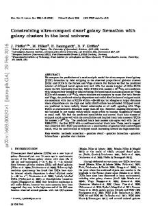
Fig. 1. Power spectra for the eleven models considered in this paper. All models are normalized to the four-year COBE data. See Table 1 for details of the models and their normalization.

(1σ) overall uncertainty (G´orski et al. 1996). The tilted model with n = 0.9 (LOWH0.9 ) is normalized assuming zero contribution from gravitational waves. The corresponding COBE–normalized power spectra for each of these eleven models are plotted in Figure 1. Several features are immediately apparent. The amount of small–scale power is decreased as Ων increases in CHDM models, or as h is lowered in CDM models. The Cν 2 DM model has less power on the cluster scale than the CνDM model with the same Ων = 0.2. The ΛCDM models have somewhat less small-scale power than the SCDM model, but also much more large–scale power. Table 1 also has a second σ8 column, which gives the values actually used for the TZA simulations. As discussed in the previous subsection, for models 11

with COBE σ8 > 1, we use a smaller value in the TZA simulations to avoid excessive non–linear effects. For all the Ω = 1 models except SCDM, this σ8 corresponds to a9 = 7.0 µK, which is consistent with the one–year COBE normalization (Smoot et al. 1992). As for the ΛCDM models, σ8 was simply set equal to 0.80 for the TZA calculations. This procedure is not expected to represent a limitation, thanks to the above–mentioned stability of the cluster clustering against changes in the spectrum amplitude. In the discussion of the cluster abundance in §5, we use the four-year COBE normalization given in Table 1.

3.3 Extraction of mock samples

We generate a parent population of clusters within the simulation box, by using dcl = 35 h−1Mpc for their average separation which corresponds to that of the ACO cluster sample. We therefore obtain, within each simulation box, the positions and peculiar velocities of 6114 clusters. Since the limiting depth of the Abell/ACO sample is much smaller than our simulation box size, we can identify more than one independent (or nearly independent) observer, in each simulation. In fact, we maximize the number of such observers to eight by placing them along the main diagonal axes of the cube. Each observer is located at a distance of 160 h−1Mpc from the boundary of the box (i.e., at a distance of ≃ 277 h−1Mpc from the nearest corner). The periodic boundary conditions in the 640 h−1Mpc simulation box allow us to periodically replicate this box as required so that each observer can define the cluster sample up to the same depth, 240 h−1 Mpc, of the observational catalogue. In order to minimize the overlapping between mock samples extracted in the same box, the coordinate system for each observer is such that its “galactic” plane is defined to be orthogonal to the one of the other three nearest observers. Since we exclude the portion of the sky with |b| ≤ 30◦ , there is only a modest overlap between neighbouring samples. We find that typically only 5% of the clusters are selected twice in each box. Finally, once the position of an observer is fixed, velocities of the clusters are used to convert the surrounding cluster distribution to redshift space. Since we have run six realizations for each model with eight observers per realization, we end up with 48 observers, which sample almost independent volumes. This is a rather large ensemble on which we can estimate the effects of cosmic variance. Once the geometry of the sample boundary has been fixed, the membership of clusters within each of the samples is decided on the basis of a Monte Carlo rejection method, which reproduces the same selection effects [i.e., the Galactic absorbtion of eq.(4) and the redshift extinction of eq.(5)] as in the real sample. Since the cluster number density is fixed in the whole 12

Table 1 The DM models. Column 1: the name of each model considered in this paper. Column 2: the density parameter Ω0 . Column 3: the percentage of the hot component Ων . Column 4: the percentage of baryons Ωbar . Column 5: the Hubble parameter h (in units of 100 km s−1 Mpc−1 ). Column 6: the age of the Universe t0 . Column 7: the rms Quadrupole amplitude for the power spectrum considered. Column 8: the corresponding rms fluctuation amplitude within a top–hat sphere of 8 h−1 Mpc radius σ8 . Column 9: the actual value of σ8 used in the TZA simulations.

Model

Ω0

Ων

Ωbar

%

%

h

t0

Qrms−PS

σ8

Gyrs

σ8 TZA

CDM models SCDM

1.0

0

5.0

0.5

13.0

17.5

1.19

1.14

LOWH

1.0

0

7.8

0.4

16.3

17.5

0.89

0.84

LOWH0.9

1.0

0

7.8

0.4

16.3

19.0

0.72

0.68

CHDM models CνDM0.1

1.0

10

5.0

0.5

13.0

17.5

0.92

0.89

CνDM0.2

1.0

20

5.0

0.5

13.0

17.5

0.80

0.77

Cν 2 DM0.2

1.0

20

5.0

0.5

13.0

17.5

0.72

0.69

CνDM0.3

1.0

30

5.0

0.5

13.0

17.5

0.74

0.71

CνDM0.5

1.0

50

5.0

0.5

13.0

17.5

0.69

0.66

ΛCDM models ΛCDM0.3

0.3

0

2.6

0.7

13.5

20.6

1.06

0.80

ΛCDM0.4

0.4

0

3.5

0.6

14.5

19.2

1.00

0.80

ΛCDM0.5

0.5

0

3.5

0.6

13.5

18.4

1.13

0.80

simulation box, variations in the number of cluster members in each sample are expected. We do not attempt to reproduce in each mock sample the exact number of clusters as in the real one. However, we distinguish the Abell and ACO portions of the sample volume and degrade randomly the number of Abell–like clusters, in order to reproduce the same relative number density variations between the Abell and ACO cluster samples [cf. eq.(6)]. Furthermore, we generate for each observer 10 mock samples, based on dif13

LOWH 8000 6000

8000 6000

4000

4000

2000

2000

Abell/ACO

1000 10

20

30

1000 10

40 50 60

20

30

40 50 60

20

30

40 50 60

SCDM

8000 6000

8000 6000

4000

4000

2000

2000

1000 10

20

30

1000 10

40 50 60

Fig. 2. The J3 (R) integral for the Abell/ACO sample (filled circles) and for Ω0 = 1 simulated models (open symbols). Errorbars for simulations correspond to the 1σ scatter over the ensemble of 48 observers (see text).

ferent random realizations of the same selection functions. This allows us to check whether variations of our results due to this effect are significant or not. We have verified that they are always smaller (by a factor > ∼ 2.5) than the observer–to–observer (i.e., cosmic variance) scatter. Note that the final results for each observer are taken as the average over these 10 different realizations of the selection functions.

4

Analysis and results

In this section we compare the results of the statistical analyses that we applied to both Abell/ACO and simulated data sets. We will deal with correlation 14

statistics, probability density functions (PDF) and percolation analysis.

4.1 The correlation analysis In order to provide a robust analysis of the cluster correlation properties, we estimate the quantity 1 J3 (R) = 4π

ZR

ξ(r) d3r ,

(7)

0

which is the integral of the two–point correlation function, ξ(r), within a sphere of radius R. According to eq.(7), if we model the two–point correlation function with the power–law ξ(r) ∝ r −γ , then J3 (R) ∝ R3−γ . Therefore, J3 (R) is expected to grow as long as ξ(r) > 0, while its flattening is the signature for a rapid declining of the two–point function. BPCM showed that the integral nature of J3 (R) makes it a reliable and stable clustering diagnostic. We estimate J3 (R) by cross–correlating the cluster positions of real and simulated samples with those of random samples using the estimator: R3 J3 (R) = 3

DD · NR2 −1 , RR · ND2 !

(8)

where DD and RR are the number of data–data and random–random pairs, respectively, having separation ≤ R and NR and ND are the numbers of the random and real clusters, respectively. We compute the value of RR by using 200 random samples having the same selection functions as the reference real sample and NR = 3000. The resulting J3 (R) for Abell/ACO clusters (filled circles) are compared in Figures 2 and 3 to Ω0 = 1 and ΛCDM models, respectively (open symbols). The reported simulation errorbars correspond to the 1σ cosmic scatter over the ensemble of 48 model observers. From this plot one may judge the reliability of a model according to the distance between the Abell/ACO data and the simulation errorbars. In order to provide a more quantitative measure of the reliability of a model, we estimate the probability that the observed Abell/ACO value, J3obs , is produced by chance, due to cosmic variance fluctuations. To this purpose, let J3i 1 P i be the measure of the i–th observer (i = 1, . . . , 48) and J¯3 = 48 i J3 be the average value. Then, let N be the number of observers for which J3i ≥ J3obs (J3i ≤ J3obs ) in a DM model for which J¯3 ≤ J3obs (J¯3 ≥ J3obs ). Therefore, the smaller the number N of such observers, the smaller the probability that a 15

SCDM

8000 6000

8000 6000

4000

4000

2000

2000

1000 10

20

30

1000 10

40 50 60

20

30

40 50 60

Fig. 3. The same as in the previous figure, but for ΛCDM models. Also reported for reference in the right panel is the result for SCDM.

measure as discrepant as J3obs is produced by chance, the larger the confidence level to which the model can be ruled out. The values of N at R = 19.4 h−1Mpc and 35.3 h−1Mpc are reported in Table 2, along with the corresponding J3 (R) values (note that these two fiducial scales nearly correspond to the correlation length and the mean separation for Abell/ACO clusters). We also show the values of J3 for the Abell/ACO sample, along with the corresponding uncertainties which are the 1σ scatter over an ensemble of 200 bootstrap resamplings (e.g., Ling, Frenk & Barrow 1986). All such results consistently indicate that CDM models produce in general too small J3 (R) values. Lowering the Hubble parameter to h = 0.4 (LOWH) and slightly tilting the primordial spectral index to n = 0.9 (LOWH0.9 ) gives −1 some improvements with respect to SCDM only on scales R< ∼ 20 h Mpc. On −1 the other hand, for R> ∼ 30 h Mpc the correlations remain too weak and no observer in these three models measures a J3 value as large as the Abell/ACO one. As for the Cold+Hot DM models, it turns out that 0.2< ∼ Ων < ∼ 0.3 is required to fit the data, quite independently of whether the hot component is shared by one or two massive neutrinos. Lowering further Ων reproduces the SCDM results on large scales. Vice versa, larger values of Ων generate an excess −1 clustering on scales R< ∼ 30 h Mpc, being consistent with real data only on the largest scales. As for the ΛCDM case, we find that all the three considered models are quite consistent with the observational constraints, with only the ΛCDM0.5 being disfavoured by its small J3 value on large scales.

16

Table 2 Clustering tests. Columns 2 and 4: value of J3 (in units of 103 ) at R = 19.4 h−1 Mpc and 35.3 h−1 Mpc respectively. Columns 3 and 5: number N of the 48 observers which measure a J3 value at least as different as the observational value, J3obs , from the simulation observer–averaged value, J¯3 (see text). Column 6: the shape parameter Γ defined by eq. (15). Column 7: the effective spectral index neff at the R = 20 h−1 Mpc scale. Column 8: probability Pχ2 for model PDFs, estimated at Rsm = 20 h−1 Mpc, to have the Abell/ACO PDF as parent distribution. Column 9: reduced skewness S3 of the smoothed cluster distribution, with Rsm = 20 h−1 Mpc.

Model

J3 (19.4)

Abell/ACO

4.2 ± 0.9

N19.4

J3 (35.3)

N35.3

Γ

neff

P>χ2

10.0 ± 1.9

S3

1.8 ± 0.3

CDM models SCDM

3.1 ± 0.2

1

5.0 ± 0.5

0

0.47

−0.61

< 10−3

1.8 ± 0.3

LOWH

3.7 ± 0.2

6

6.5 ± 0.6

0

0.31

−0.83

< 10−3

1.8 ± 0.3

LOWH0.9

3.7 ± 0.2

7

6.4 ± 0.5

0

0.27

−0.91

0.002

1.8 ± 0.3

CHDM models CνDM0.1

3.9 ± 0.2

12

6.7 ± 0.5

0

0.30

−0.83

< 10−3

1.7 ± 0.2

CνDM0.2

4.5 ± 0.3

13

8.0 ± 0.6

6

0.21

−0.99

0.255

1.8 ± 0.2

Cν 2 DM0.2

4.6 ± 0.3

10

8.6 ± 0.6

9

0.19

−1.07

0.776

1.8 ± 0.3

CνDM0.3

5.0 ± 0.3

4

8.9 ± 0.6

9

0.16

−1.09

0.667

1.8 ± 0.3

CνDM0.5

5.9 ± 0.3

0

10.1 ± 0.6

25

0.11

−1.22

0.955

1.8 ± 0.3

ΛCDM models ΛCDM0.3

5.1 ± 0.3

4

9.6 ± 0.6

15

0.18

−1.15

0.997

1.8 ± 0.3

ΛCDM0.4

4.7 ± 0.3

8

8.7 ± 0.6

9

0.20

−1.09

0.991

1.8 ± 0.3

ΛCDM0.5

4.0 ± 0.2

18

7.1 ± 0.6

2

0.26

−0.94

0.212

1.8 ± 0.3

4.2 The PDF statistics

The probability density function (PDF), P (δ), for the density fluctuation field is defined as the probability for that field to assume a given value δ. Although it provides the lowest–order (i.e., 1–point) statistical description, it conveys 17

information about moments of the density field of any order, via Z

hδ q i =

P (δ) δ q dδ

(9)

with h δ i = 0 by definition. Eq.(9) defines the variance and the skewness of the δ–field for q = 2 and q = 3, respectively, while S3 = h δ 3 i/hδ 2 i2 is the reduced skewness. Several models have been proposed for P (δ) on the basis of different approaches to the description of non–linear gravitational clustering (see, e.g., Sahni & Coles 1995 and references therein). Several authors attempted recently to apply the PDF statistics to test such clustering models, using N– body simulations (e.g., Bernardeau & Kofman 1995), as well as the actual galaxy (e.g., Kofman et al. 1994) and the cluster (Plionis & Valdarnini 1995) distributions. Here we are only interested in comparing the PDF statistics for the Abell/ACO sample to that of the simulations to put constraints on DM models. In order to obtain a continuous field from the discrete cluster distribution we resort to the same smoothing procedure that has been applied by Plionis & Valdarnini (1995; see also Plionis et al. 1995 and BPCM). It can be summarized as follows. (a) We smooth the cluster distribution by using the Gaussian kernel W(r) =

2 (2πRsm )−3/2

r2 exp − 2 2Rsm

!

.

(10)

(b) We reassign the density on a grid with 20 h−1Mpc spacing according to the relation ρ(xg ) =

P

i

wi W(|xg − xi |) R . W(r) d3 r

(11)

In the above equation, xg and xi represent the vector positions for the grid point and for the i–th cluster, respectively, while wi is the weight assigned to the i–th cluster. Since we sum up over clusters such that |xg − xi | ≤ 3Rsm , the integral in the denominator takes a value slightly smaller than unity (≃ 0.97). (c) We consider only those grid points whose position corresponds to a value of the completeness factor, f (xg ) ≥ 0.8, where f (xg ) ≈ [P (z) P (b)]−1 ; for the proper definition of f see Plionis & Valdarnini (1995). It is clear that, since the parent cluster distribution has a discrete nature, the statistics of the smoothed field will be affected by shot–noise effects. However, we prefer not to correct for such effects. Firstly, the usual shot–noise 18

0.2

0.2

0.15

0.15

0.1

0.1

0.05

0.05

0 -1

0

1

0 -1

2

0.2

0.2

0.15

0.15

0.1

0.1

0.05

0.05

0 -1

0

1

0 -1

2

0

1

2

0

1

2

Fig. 4. The probability density function (PDF) for the cluster density field smoothed with a Gaussian window of 20 h−1 Mpc radius for SCDM, LOWH0.9 , Cν 2 DM0.2 and ΛCDM0.5 . The dashed line is the result for the Abell/ACO sample, while the dashed band is the 1σ “cosmic” scatter for the simulation PDFs.

corrections (e.g., Peebles 1980) are based on the assumption that the point distribution represents a Poisson sampling of an underlying continuous field whose statistics one is wishing to recover. This is clearly not the case for the distribution of clusters, which are instead expected to trace the high density peaks of the DM density field (see e.g. Borgani et al. 1994). Secondly, our simulation cluster samples are constructed to have the same number density as the Abell/ACO sample. Therefore, shot–noise should affect similarly the simulation and real data analysis, and thus we will be comparing like with like. Furthermore the smoothing process itself suppresses significantly the shot– noise effects (Gazta˜ naga & Yokoyama 1993) and thus we will consider only 19

Rsm ≥ 20 h−1 Mpc for the smoothing radius. BPCM showed that the PDF statistics at Rsm = 20 h−1Mpc are effective in discriminating between different DM models, while the weak cluster clustering makes such differences hardly detectable at Rsm = 30 h−1Mpc. For this reason, we will present in the following only results based on the smaller Rsm value. As an example, we plot in Figure 4 the PDFs for some models and compare them with the Abell/ACO results (dashed curve). For model PDFs, the shaded band represents the 1σ scatter estimated over the 48 observers. Between the four plotted models, it is apparent that the SCDM is the most discrepant; the weakness of the clustering produced by this model turns into a PDF shape which is significantly broader that the Abell/ACO one. In order to provide a quantitative comparison, we also estimate the quantity

χ2 =

X i

"

P sim(δi ) − P obs (δi ) σi

#2

,

(12)

where the index i runs over the bins in δ and σi2 is the cosmic variance in the determination of P sim (δ). In Table 2 we report the probability P>χ2 that the simulation PDF could have been drawn by chance from a parent distribution given by the observational PDF. The results confirm what we found from the J3 analysis: all the CDM models with Ω0 = 1 and the CνDM0.1 one are rejected at a quite high confidence level. The only exception is the CνDM0.5 model, which is now perfectly acceptable. However, these results are obtained for a Gaussian window of radius Rsm = 20 h−1 Mpc, which roughly corresponds to R ≃ 35 h−1 Mpc for the radius of the top–hat sphere on which the J3 test is based. Therefore, this result is consistent with the agreement between Abell/ACO and CνDM0.5 analyses at that scale. As in BPCM we have found that the value of the reduced skewness S3 (see Column 4 of Table 2), is remarkably independent of the model and virtually identical to that characterizing the Abell/ACO clusters (see also Gazta˜ naga, Croft & Dalton 1995; Jing, B¨orner & Valdarnini 1995). This indicates that S3 is not connected to the fluctuation spectrum but either to the nature (i.e., Gaussian vs. non–Gaussian) of the initial fluctuations or to the high–peak biasing prescription for identifying clusters. In any case, the remarkable agreement between data and all the model predictions indicates that the Abell/ACO clusters are consistent with being high density peaks of a mildly non–linear density field, evolved according to the gravitational instability picture from random–phase initial conditions (cf. also Kolatt, Dekel & Primack 1996).

20

4.3 The percolation analysis

Different but complementary information can be obtained by using a percolation technique, essentially based on the friends–of–friends algorithm. In fact this method allows one to individuate the largest structures present in the cluster samples, roughly corresponding to supercluster sizes. Percolation, as a discriminatory tool between different cosmological models, has been criticized due to the dependence of the results on the mean density of the objects and/or on the volume sampled (e.g. Dekel & West 1985). For these reasons we checked the stability of the following results against possible small changes in the parameters of the simulated catalogues (the mean separation dcl , the ratio between the number density of Abell and ACO cluster samples, the parameters of the selection function, etc.). Although, by varying these parameters the final number of clusters inside the simulated catalogues can vary up to 30%, we found that all the main results are robust, showing variations smaller than the observer–to–observer variance. As a first statistical test, we compute the fraction of clusters in superclusters as a function of the percolation radius Rp (Postman et al. 1989; Plionis, Valdarnini & Jing 1992, hereafter PVJ), where a supercluster is defined as a group with a number of members Nm ≥ 2. The results for the different cosmological models are shown in Figure 5, where the behaviour of this statistics for the real sample is also plotted (filled circles). The errorbars, centred on the real data, are the 2σ errors in the observer’ ensemble for the SCDM model: very similar error sizes are obtained for the other models. The results are in good agreement with those obtained by our previous analyses. The SCDM model has a small fraction of clusters inside the superclusters for percolation −1 radii Rp < ∼ 30 h Mpc. This agrees with the results of the correlation analysis, which indicates a lack of close cluster pairs in the SCDM model. On the other hand, the Cold+Hot DM models with Ων = 0.5 forms superclusters too easily, with a consequent too large fraction of clusters in superclusters. The other models are all well inside the 2σ errorbars, with some exceptions at very small percolation radii (Rp ≤ 12 h−1 Mpc). This discrepancy is essentially due to the fact that our simulation method is not suitable to resolve the very close pairs of clusters, reducing systematically the percolation at these small radii. As a further test, we compute the multiplicity function MF (i.e. the number of superclusters with a given cluster membership Nm ) at two different percolation radii, Rp = 20 and 35 h−1 Mpc: these two values have been chosen to approximate the cluster correlation length and the mean intercluster separation, respectively. In order to decrease the shot–noise effects and thus to perform a reliable statistical analysis, we prefer to bin our results in logarithmic intervals; we tested that the final results are almost independent of the 21

Fig. 5. The fraction of clusters in superclusters as a function of the percolation radius Rp (in h−1 Mpc). The filled circles refer to the Abell/ACO clusters, while the corresponding values for the different models are represented by the different lines. The errorbars, centred on the real data, are the 2σ scatter estimated over the ensemble of observers for the SCDM model. The panels refer to the CDM models (top), the CHDM models (centre) and the ΛCDM models (down).

choice of the binning parameters. We compare the MF of the real sample to that of each simulated catalogue by using a χ2 –test. In Table 3 we report, for both percolation radii, the fraction FM F of the 480 simulated catalogues (corresponding to the 10 selection function realizations for each of the 48 observers) of each model with a χ2 probability of reproducing the real data which is larger than 0.15. Although some differences exist between the models, the 22

fraction of such “good” observers is very large for all the models (> 0.8) which indicates that the MF is not a discriminatory test. As a consequence, all the models agree with the observational data. The shapes of the superclusters have been suggested as a useful tool to discriminate among different models (see, e.g., Matarrese et al. 1991; PVJ). This statistics is based on the computation for each supercluster of the inP ertia tensor Ikl = N i=1 (Xk Xl )i Wi , where the indices k and l range from 1 to 3, and X1i , X2i , X3i are the cartesian coordinates of the i–th cluster computed with respect to the centre of mass of the supercluster. In order to reduce the importance of the outlying clusters, we weight each cluster by Wi = (X12i +X22i +X32i )−1 , which is the inverse square cluster distance from the supercluster centre of mass (West 1989; PVJ). We then compute the following three quantities, λ1 = 1/a23 , λ2 = 1/a22 and λ3 = 1/a21 , where a21 ≥ a22 ≥ a23 are the eigenvalues of the principal axes of the inertia tensor. Following Bardeen et al. (1986), we define for each supercluster two shape parameters: e=

λ1 − λ3 ≥0 P 2 3i=1 λi

(13)

and p=

λ1 − 2λ2 + λ3 . P 2 3i=1 λi

(14)

The quantity e is a measure of the ellipticity in the λ1 − λ3 plane while p measures the prolateness (if −e ≥ p ≥ 0) or oblateness (if 0 ≥ p ≥ e) of the supercluster. The limiting cases p = −e and p = e represent the prolate and oblate spheroid, respectively. In order to have reliable statistical characterization of supercluster shapes, we need at the same time a large number of such structures, each containing a rather large number of members. For this reason, we consider in this analysis all the simulated superclusters with Nm ≥ 9. In Figure 6 we show the distributions of values of e and p obtained for SCDM, Cν 2 DM and ΛCDM0.5 models, when a percolation radius of Rp = 35 h−1Mpc is adopted (similar results have been obtained for the other models and are not reported). The solid lines represent the isoprobability contours while the dashed lines show the triangle where the values of e and p are constrained to lie. The results for the nine Abell/ACO superclusters are displayed as filled symbols (in the upper panels, circles are for the two superclusters with Nm ≥ 40, squares for Nm < 40). The behaviour for the different models is very similar: the shapes are systematically triaxial, with a tendency to oblateness. Moreover we find, in agreement with previous analyses (Matarrese et al. 1991; PVJ) and with theoretical predictions for a Gaussian random field (e.g., Bardeen et al. 1986), 23

Fig. 6. Comparison of the shape parameters e and p for the observed and the simulated superclusters found with a percolation radius Rp = 35 h−1 Mpc. Only the SCDM (left panels), Cν 2 DM0.2 (central panels) and ΛCDM0.5 (right panels) models are reported here. Upper and lower panels are for superclusters with Nm ≥ 9 and Nm ≥ 40, respectively. The dashed lines represent the triangle where the values of e and p are constrained to lie. The solid lines refer to the isoprobability contours: the spacing is 0.004 starting from the external contour referring to a probability of 0.004. The real data are represented by filled circles, if the number of members is Nm ≥ 40, or filled squares, if 9 ≥ Nm < 40.

that the richer superclusters have the tendency to be more spherical than the poorer ones. In general we find that the parameter values obtained for the real superclusters are rather typically reproduced by all models. In Table 3 we report the fraction Fobl of superclusters having an oblate shape, i.e. with p ≥ 0, computed for a percolation radius of both 20 and 35 h−1 Mpc, for both real and simulated samples. We note that, since a total number of only 6 superclusters characterizes the statistics of the Abell/ACO sample, the corresponding Poissonian uncertainties are so large that all the models are in agreement with the results for the real sample. Furthermore, we also report in Table 3 the number of clusters inside the richest max supercluster, Nm , computed for two values of the percolation radius, Rp = 20 −1 and 35 h Mpc, along with the 1σ scatter within the observer’ ensemble. At the smaller Rp , the only models which do not agree with the Abell/ACO result are the SCDM, both the LOWH models and, more marginally, CνDM0.1 , which 24

produce too poor superclusters. On the other hand, the much larger cosmic variance at Rp = 35 h−1Mpc does not allow to detect any significant difference between the models. Therefore, combining the results about the multiplicity function with those max from Nm , we conclude that Cold+Hot DM models with Ων = 0.2–0.3 and the considered ΛCDM models reproduce rather well the percolation properties of the Abell/ACO cluster sample, thus in agreement with the constraints obtained from the previous analyses.

5

Discussion

5.1 Spectrum shape The results that we presented in the previous section converge to indicate that the cluster distribution is indeed a powerful tool to constrain different power spectrum models. The results reported in Table 2 show that the statistics of the cluster distribution is quite sensitive to the power spectrum shape, while independent analyses (e.g., Croft & Efstathiou 1994; BPCM) show that the amplitude of the cluster correlations in a given model is almost independent of the normalization or evolutionary stage. In order to understand in more detail the constraint that the cluster distribution provides on the spectrum profile of cosmological models, we decided to correlate the cluster J3 values with suitable parameters defining the profile of P (k). In particular, we considered the shape parameter defined by Γ = 0.5



0.95σ8 3.5σ25

1/0.3

= 0.3826(EP )−1/0.3 ,

(15)

(σ8 and σ25 are the rms fluctuation amplitudes within top–hat spheres of 8 h−1 Mpc and 25 h−1Mpc radii, respectively) and the effective spectral index neff = −3 −

d log σ 2 (R) . d log R

(16)

With the definition (15), for SCDM and the ΛCDM models the shape parameter is approximately equivalent to the quantity Γ = Ω0 h exp(−Ωbar −Ωbar /Ω0 ), which specifies the CDM transfer function (Efstathiou, Bond & White 1992), suitably corrected to account for a non–negligible baryon contribution (Peacock & Dodds 1994; Sugiyama 1995). In eq. (15), the “Excess Power” EP ≡ 25

Table 3 Percolation tests. The fraction FM F of simulated catalogues having a χ2 probability of reproducing the observed multiplicity function larger than 0.15; the fraction Fobl max inside the of superclusters having an oblate shape; the number of clusters Nm richest supercluster.

Model

FM F

Fobl

max Nm

perc. radius Rp = 20 h−1 Mpc

Abell/ACO

0.667

17

FM F

Fobl

max Nm

perc. radius Rp = 35 h−1 Mpc

0.889

85

CDM models SCDM

0.817

0.854

11.3 ± 2.3

0.735

0.830

93.4 ± 31.7

LOWH

0.873

0.884

12.9 ± 3.1

0.792

0.820

92.1 ± 36.2

LOWH0.9

0.896

0.879

12.9 ± 2.8

0.786

0.839

96.0 ± 36.3

CHDM models CνDM0.1

0.915

0.867

13.2 ± 3.6

0.746

0.820

90.7 ± 33.3

CνDM0.2

0.933

0.879

14.7 ± 4.8

0.819

0.832

89.8 ± 28.5

Cν 2 DM0.2

0.980

0.881

15.4 ± 5.1

0.800

0.837

92.3 ± 30.2

CνDM0.3

0.954

0.888

15.3 ± 4.0

0.813

0.835

89.6 ± 29.5

CνDM0.5

0.960

0.876

18.1 ± 5.1

0.798

0.854

86.8 ± 27.4

ΛCDM models ΛCDM0.3

0.931

0.882

16.9 ± 4.7

0.860

0.844

104.4 ± 41.3

ΛCDM0.4

0.921

0.868

15.4 ± 4.4

0.829

0.851

101.0 ± 37.5

ΛCDM0.5

0.865

0.882

14.5 ± 3.8

0.827

0.830

97.4 ± 31.4

3.4σ25 /σ8 , defined so that SCDM has EP ≈ 1, was introduced by Wright et al. (1992), who stated that EP ≈ 1.3 is needed to fit the APM galaxy angular correlation function; with the above definition, this corresponds to Γ ≈ 0.16. We plot in Figure 7 the J3 values at R = 20 h−1Mpc for each model versus the corresponding Γ (left panel) and neff (right panel) values. We decided not to include plots of results for larger scales, for which we have already verified that the results are less discriminatory. The values of Γ and neff for all the 26

6000

6000

5000

5000

4000

4000

3000

3000 0.1

0.2

0.3

0.4

0.5

-1.2

-1

-0.8

-0.6

Fig. 7. The value of the J3 integral for all the models evaluated at R = 20 h−1 Mpc is plotted against the value of the corresponding shape parameter Γ (left panel) and effective spectral index, neff evaluated at the same scale. The horizontal dotted line is the J3 value for the Abell/ACO sample.

models have been already reported in Table 2. Apart from the individual model details, the correlation between the spectrum shape and the J3 values is really striking: the steeper the spectrum, the stronger the cluster correlations, with the extreme two models being CνDM0.5 and SCDM. The trends are especially clear if one compares models of the same class, represented in Figure 7 by points of the same shape. The dashed line connects the four CνDM models and SCDM, obtained by varying Ων from 0.5 to 0. The Cν 2 DM model lies only slightly below this dashed line. The fact that J3 shows the same trend as a function of nef f or of our generalized Γ shape parameter shows that these characterize well the behaviour of the cluster correlations. A comparison with the J3 result for the Abell/ACO sample (horizontal dotted −1 lines) leads to 0.18< ∼ Γ< ∼ 0.25 and −1.1< ∼ neff < ∼ − 0.9 at R ≃ 20 h Mpc being required by the cluster distribution. It is interesting to note that this value of Γ agrees with that, Γ = 0.23 ± 0.04, obtained by Peacock & Dodds (1994) from the power spectrum analysis of APM galaxies (cf. also Viana & Liddle 1995). This suggests that optical galaxies and Abell/ACO clusters actually trace the same power spectrum, at least on such scales, the only difference arising from their different linear biasing factors. Recently Eke et al. (1996b) considered SCDM cluster N–body simulations in order to check the stability of the cluster clustering when different prescription for their identification are applied. Although they found rather marginal differences, it is clear that 27

realistic cluster identification methods in simulations should be considered when new observational cluster samples based on improved selection criteria will be available.

5.2 Spectrum amplitude Although the statistics of the cluster distribution represents a useful tool for providing hints about the shape of the power spectrum, nevertheless one may well imagine that different combinations of the fundamental parameters which enter in defining a model (i.e., DM composition, values of Ω0 , ΩΛ and h) could produce the same profile of the transfer function. For this reason, further observational tests are required to constrain also the fluctuation amplitude, which is expected to vary from model to model, due to the different way in which the defining parameters enter in specifying the large–scale normalization to CMB temperature fluctuations. The most constraining of such tests is probably the abundance of galaxy clusters (see, e.g., White, Efstathiou & Frenk 1993; BPCM; Viana & Liddle 1995; Eke, Cole & Frenk 1996a; Borgani et al. 1996a,b, and references therein). Since our TZA simulations are inadequate to describe mass accretion into clusters, we resort here to the analytical approach provided by Press & Schechter (1974, PS). According to this recipe, the number density of collapsed structures of mass larger than M is N(> M) =

Z∞

n(M ′ ) dM ′ .

(17)

M

Here, n(M) dM is abundance of structures with mass between M and M +dM, which reads n(M) dM =

s

2 ρ¯δc π σM

δ2 exp − c2 d log M 2σM

d log σM

!

dM , M2

(18)

where ρ¯ is the average cosmic density, δc is the critical density contrast for a linearly evolved overdensity to turn into a collapsed structure, and σM =



1/2 1 Z 2 2 P (k) W (kR) k dk 2π 2

(19)

is the rms mass fluctuation within the window W (kR). As usual, the mass M is connected to the window radius R according to M = f R3 , f being a form 28

factor, which depends on the W profile. For the Gaussian window W (kR) = exp(−k 2 R2 /2) that we will consider in the following, it is f = (2π)3/2 . As for the δc value, linear theory for spherical top–hat collapse predicts δc = 1.69 (e.g., Peebles 1980). However, deviations from this value are expected on several grounds. For instance, asphericity of the collapse would in general predict a lower δc (e.g., Monaco 1995). Such an effect is generally believed to be of limited relevance, since exceptionally high peaks are expected to closely follow a spherical collapse (e.g., Bernardeau 1994). It is however not clear whether this high–peaks approximation would apply to real clusters. Indeed, for models with σ8 ≃ 0.8 and δc ≃ 1.7, clusters would arise just from ≃ 2σ overdensities of the initial linear field. From N–body simulations of the CνDM0.3 model, Klypin & Rhee (1994) and Walter & Klypin (1996) found that eq.(18) with δc ≃ 1.5 and Gaussian window provides a good fit to the resulting cluster mass function. Although the stability of this result when changing the DM model should be still understood in detail, it is well established that linear–theory predictions for δc do not depend strongly on the value of Ω0 (e.g., Lilje 1992; Lacey & Cole 1993; Colafrancesco & Vittorio 1994). This has been been confirmed by the N–body approach followed by White et al. (1993) for CDM–like models with Ω0 = 0.2 and Ω0 = 1 (cf. also Mo et al. 1996). We show in Figure 8 the results of some new N–body simulations undertaken just to clarify this point, and also the dependence on the precise definition of the region regarded as the cluster, defined either by the Abell radius 1.5h−1 Mpc, or by the radius at which the overdensity falls below 200 (the latter is larger for rich clusters). These N–body results are from PM simulations with a 5123 force mesh and 2563 particles in a 200 h−1 Mpc box. The mass functions constructed for model (a) are for just a single realization, while model (b) is an average of three realizations, and model (c) is the average of two realizations 1 . The upper and lower asterisks in the figure represent the observational data points of Biviano et al. (1993) and White et al. (1993). For cluster mass in 1

Note that the normalization of model (a) is lower than that in Table 1: σ8 = 1.06 there, while σ8 = 0.90 for this simulation. Such a low normalization has been advocated by some authors to avoid the excess power on small scales calculated for this model by Klypin et al. (1996). But our results in Panel (a) confirm that the cluster abundance with this lower model normalization is lower than the observations indicate, according to White et al. (1993) and Biviano et al. (1993). Models (b) and (c) are also different from the ΛCDM0.4 model considered in this paper, since the spectra are slightly tilted (n = 0.975 or 0.90 with T /S = 0). However, the results are consistent with our PS calculations presented in Figure 9. For example, if a PS curve were plotted for model (c) in Figure 9, it would cross the middle of the dark shaded band at δc = 1.3. The tilted ΛCDM0.4 model (c) is being investigated further by Klypin et al. (in preparation) as an example of a ΛCDM model that might avoid the problem of too much power on small scales.

29

(a)

(b)

(c)

Fig. 8. The abundance N (> M ) of clusters as a function of mass M , comparing results from Press–Schechter theory with those from N–body simulations for three ΛCDM models: (a) Ω0 = 0.3, h = 0.7, n = 1, and σ8 = 0.9; (b) Ω0 = 0.4, h = 0.6, n = 0.975, and σ8 = 1.0; (c) Ω0 = 0.4, h = 0.6, n = 0.9, and σ8 = 0.87. Dashed lines are for Press-Schechter (PS) approximations for the models. The short dashed line represents PS with a Gaussian filter and δc = 1.3. The long dashed line represents PS with a top-hat filter and δc = 1.68. The solid and dotted lines are for mass functions (MFs) from simulations. Solid lines are for MFs that have been constructed from halos defined by the spherical radius at which the overdensity falls below 200. Dotted lines are for MFs that have been constructed from halos defined by the spherical Abell radius of 1.5h−1 Mpc. The upper star symbol on each panel represents the observational data point of Biviano et al. (1993), and the lower one is that of White et al. (1993). See text for discussion.

30

the region of these observational data points, the mass function fluctuates by about 10% from the average value from realization to realization. From the results shown, it appears that the Press-Schechter approximation with a Gaussian filter and δc = 1.3 is a good fit to the mass function from simulations. This PS fitting function is very similar in shape to the one obtained with a top-hat filter and the canonical δc = 1.68. In general, both of these PS curves fit the mass functions from simulations with the R200 definition reasonably well and the mass functions with the RAbell definition very well. The only clear exception is in the case of model (a) where the RAbell definition is significantly below the PS curves and the data points. However, by nature this model has fewer massive clusters than the others, so the steep decline at the high-mass end of the curve may be due to statistical fluctuation caused by poor counting statistics. Note that model (c), which best fits the 0.53−0.13(1−Ω0 ) cluster abundance data points, has σ8 Ω0 = 0.56, thus somewhat larger than the value 0.50 ± 0.04 obtainable for the Eke et al. (1996a) results for this model. We can summarize the discussion above by saying that for CHDM models there is a good fit to the cluster abundance with δc = 1.5 in PS with a Gaussian filter, and for ΛCDM models δc = 1.3 gives a good fit. In order to have a rather conservative approach, we prefer to work out predictions of the cluster abundance for all the models we consider for a range of δc values (see also BPCM), 1.3 ≤ δc ≤ 1.7. In Figure 9 we plot N(> M) as a function of δc for all the models, assuming M = 4.2 × 1014 h−1 M⊙ . This value for the limiting mass is that at which White et al. (1993) report cluster abundances from X–ray and velocity dispersion data. Note that larger values of M ≃ 1015 h−1 M⊙ would sample the mass function on its high–mass exponential tail, where any uncertainty in the mass determination would affect N(> M) more. The shaded band in Figure 9 indicates the observational results; it is delimited from below by the X–ray based abundance by White et al. (1993), and from above by the determination by Biviano et al. (1993), based on cluster velocity dispersions. Although realistic observational uncertainties are probably larger than the difference between such results, it is not clear whether they can account for the large discrepancies displayed by some models. For instance, even if cluster masses from X–ray data were underestimated by a factor of two (cf. Balland & Blanchard 1995; see, however, Evrard, Metzler & Navarro 1996, for arguments in favour of a precise mass determination), the SCDM prediction would decrease to N(> M) ≃ 1.8 × 10−5 , still quite far from the observational result. The four panels of Figure 9 correspond to different ways of lowering the SCDM prediction of N(> M): (a) introducing a hot component; (b) sharing Ων between more massive neutrinos; (c) lowering h and/or tilting the primordial P (k); (d) lowering Ω0 , still keeping flatness. Note that increasing to some extent the baryon fraction would also decrease N(> M). In view of such uncertainties in both the observational outputs and the values of the 31

0.0001

0.0001

SCDM

1.3

1.4

1.5

SCDM LOWH

1.6

1.7

0.0001

1.3

1.4

1.5

1.6

1.7

1.6

1.7

0.0001

SCDM

1.3

1.4

1.5

1.6

1.7

1.3

1.4

1.5

Fig. 9. The abundance N (> M ) of clusters having mass larger than M = 4.2×1014 h−1 M⊙ arising from the Press–Schechter theory, plotted as a function of the critical density contrast, δc . Results are obtained by adopting a Gaussian window function. The dashed band is delimited from below by the observational result of White et al. (1993) and from above by that of Biviano et al. (1993).

model parameters, we believe that it is fair to draw the following conclusions. (a) Critical density CDM models are allowed only by substantially lowering the Hubble parameter at least to h = 0.4 and/or tilting the primordial spectral index at least to n = 0.9. (b) The Cold+Hot DM model with n = 1 is required to have Ων > ∼ 0.3, with Ων ≃ 0.2 still allowed if more than one massive neutrino species share the hot contribution. A larger parameter space is allowed if the primordial spectral index is allowed to tilt slightly below the Zel’dovich value n = 1 (cf. Primack et al. 1995, 1996; Liddle et al. 1995a). (c) ΛCDM models should have Ω0 < ∼ 0.4 in order to provide a substantial 32

improvement with respect to SCDM for n = 1, with a larger parameter space available for n < 1 (Klypin et al. 1996; Liddle et al. 1995b).

6

Conclusions

In this paper we discussed extensively how the distribution of galaxy clusters can be used to constrain cosmological models for large–scale structure formation. Our reference cluster distribution is a combined redshift sample of Abell/ACO clusters. We compare this observational distribution to that predicted by a list of eleven DM models. To this purpose, we run for each model a large set of numerical simulations based on an optimized version of the truncated Zel’dovich approximation (TZA). Taking advantage of the reliability and flexibility of this simulation method, we end up with 48 independent mock samples for each model, each reproducing the same cluster number density and selection functions as the Abell/ACO one. We use this ensemble of realizations to reliably estimate cosmic variance effects. In order to assess the reliability of the considered models, we apply to both real and simulated samples several clustering analyses, like the correlation statistics based on the J3 integral, the probability density function and supercluster statistics based on percolation method. The conclusions that we draw from these analyses can be summarized as follows. (a) All the Ω0 = 1 CDM models produce too weak cluster clustering. Lowering the Hubble parameter to h = 0.4 and/or tilting the primordial spectral index to n = 0.9 does not improve the standard CDM model enough. This is true regardless of the normalization σ8 . (b) Cold+Hot DM models with 0.2< ∼ Ων < ∼ 0.3 fit the Abell/ACO data rather well, almost independent of whether the hot component is shared between one or two massive neutrino species. A model with Ων = 0.1 produces weak clustering, similar to the SCDM model. On the contrary, the Ων = 0.5 case −1 fails in that it overproduces clustering on scales < ∼ 30 h Mpc and makes clusters percolate far easier than is observed. (c) All the three considered ΛCDM models fare rather well, with the Ω0 = 0.5 case being less favoured due to the marginal lack of clustering at R ≃ 35 h−1Mpc. (d) As a general result, we find that the cluster distribution presents a constraint only for the power–spectrum shape, but not for its amplitude. Reproducing the observed Abell/ACO cluster clustering requires 0.18< ∼ Γ< ∼ 0.25 < < for the shape parameter (15), or −1.1∼ neff ∼ −0.9 for the effective spectral index (16) at the 20 h−1Mpc scale. In order to constrain also the power spectrum amplitude, we resort to the 33

estimation of the cluster abundance, which is essentially determined by σ8 , the rms linear fluctuation value within a top–hat sphere of 8 h−1 Mpc radius (e.g., White et al. 1993). Since no reliable mass determination is allowed by our TZA cluster simulations, we use the Press & Schechter (1974) approach. We think of the Press–Schechter formula as a parametric fitting to the “true” mass function, where our ignorance about the details of the non–linear gravitational clustering is accounted for by varying the critical density parameter δc in a rather broad range of values. Comparing to N–body simulations, good fits to the cluster mass function are obtained for PS with gaussian filter with δc ≈ 1.5 for CHDM models and δc ≈ 1.3 for ΛCDM models. Combining results from the analysis of the spatial distribution and the abundance of clusters it turns out that the only viable models, of those considered here, are either the Cold+Hot DM ones with 0.2< ∼ Ων < ∼ 0.3, better if shared between more than one massive ν species, or ΛCDM models with 0.3< ∼ Ω0 < ∼ 0.5 and Hubble constant tuned in such a way to give about 14 Gyrs for the age of the Universe.

Acknowledgments. SB and LM have been partially supported by Italian MURST. AK, JRP, and CLS acknowledge support from NASA and NSF grants, and the use of the CM5 at the National Center for Supercomputer Applications, University of Illinois, Urbana-Champaign.

References Abell G.O., 1958, ApJ, 3, 211 Abell G.O., Corwin H.G., Olowin R.P., 1989, ApJS, 70, 1 Achilli S., Occhionero F., Scaramella R., 1985, ApJ, 299, 577 Adams F., Bond J.R., Freese K., Frieman J.A., Olinto A., 1993, Phys. Rev. D, 47, 426 Athanassopoulos C., et al., 1995, Phys. Rev. Lett., 75, 2650 Bahcall N.A., 1988, ARA&A, 26, 631 Bahcall N.A., Cen R., 1992, ApJ, 398, L81 Bahcall N.A., Soneira R.M., 1983, ApJ, 270, 20 Balland C., Blanchard A., 1995, preprint astro-ph/9510130 Bardeen J.M., Bond J.R., Kaiser N., Szalay A.S., 1986, ApJ, 304, 15 Batuski D.J., Bahcall N.A., Olowin R.P., Burns J.O., 1989, ApJ, 341, 599 Bennett C.L., et al., 1996, ApJ, 464, L1 Bernardeau F., 1994, ApJ, 427, 51 34

Bernardeau F., Kofman L., 1995, ApJ, 443, 479 Biviano A., Girardi M., Giuricin G., Mardirossian F., Mezzetti M., 1993, ApJ, 411, L13 Blumenthal G.R., Dekel A., Primack J.R., 1988, ApJ, 326, 539 Blumenthal G.R., Faber S.M., Primack J.R., Rees M.J., 1984, Nature, 311, 517 Bonometto S.A., Valdarnini R., 1984, Phys. Lett., A103, 369 Borgani S., 1990, A&A, 240, 223 Borgani S., Coles P., Moscardini L., 1994, MNRAS, 271, 223 Borgani S., Coles P., Moscardini L., Plionis M., 1994, MNRAS, 266, 524 Borgani S., Gardini A., Girardi M., Gottl¨ober S., 1996b, in preparation Borgani S., Lucchin F., Matarrese S., Moscardini L., 1996a, MNRAS, 280, 749 Borgani S., Plionis M., Coles P., Moscardini L., 1995, MNRAS, 277, 1191 (BPCM) Branch D., Nugent P., Fisher A., 1995, Proceedings of the NATO Advanced Study Institute on Thermonuclear Supernovae, preprint astro-ph/9601006 Cen C.J., Gnedin N.Y., Kofman L.A., Ostriker J.P., 1992, ApJ, 399, L11 Colafrancesco S., Vittorio N., 1994, ApJ, 422, 443 Coles P., 1989, MNRAS, 238, 319 Coles P., Melott A.L., Shandarin S.F., 1993, MNRAS, 260, 765 Collins C.A., Guzzo L., Nichol R.C., Lumsden S.L., 1995, MNRAS, 274, 1071 Croft R.A.C., Efstathiou G., 1994, MNRAS, 267, 390 Dalton G.B., Croft R.A.C., Efstathiou G., Sutherland W.J., Maddox S.J., Davis M., 1994, MNRAS, 271, L47 Davis M., Summers F.J., Schlegel M., 1992, Nature, 359, 393 Dekel A., West M.J., 1985, ApJ, 288, 411 Doroshkevich A.G., Shandarin S.F., 1978, MNRAS, 182, 27 Efstathiou G., Bond J.R., White S.D.M., 1992, MNRAS, 258 1p Eke V.R., Cole S., Frenk C.S., 1996a, 282,263 Eke V.R., Cole S., Frenk C.S., Navarro J.F. 1996b, preprint astro-ph/960291 Evrard A.E., Metzler C.A., Navarro J.F., 1996, ApJ, 469, 494 Fang L.Z., Li S.X., Xiang S.P., 1984, A&A, 140, 77 Gazta˜ naga E., Croft R.A.C., Dalton G.B., 1995, MNRAS, 276, 336 Gazta˜ naga E., Yokoyama J., 1993, ApJ, 403, 450 Ghigna S., et al., 1994, ApJ, 437, L71 G´orski K.M., Banday A.J., Bennett C.L., Hinshaw W.G., Kogut A., Smoot G.F., Wright E.L., 1996, ApJ, 464, L11 G´orski K.M., Ratra B., Sugiyama N., Banday A., 1995, ApJ, 444, L65 Hockney R.W., Eastwood J.W., 1981, Computer Simulations Using Particles. McGraw–Hill, New York Hodges H.M., Blumenthal G.R., Kofman L.A., Primack J.R., 1990, Nucl. Phys. B, 335, 197 Holtzman J.A., 1989, ApJS, 71, 1 Holtzman J.A., Primack J.R., 1993, ApJ, 405, 428 35

Jing Y.P., B¨orner G., Valdarnini R., 1995, MNRAS, 277, 630 Jing Y.P., Fang L.Z., 1994, ApJ, 432, 438 Jing Y.P., Plionis M., Valdarnini R., 1992, ApJ, 389, 499 Katgert P., et al., 1996, A&A, 310, 8 Kennicutt R.C., Freedman W.L., Mould J.R., 1995, AJ, 110, 1476 Kerscher M., Schmalzing J., Retzlaff J., Borgani S., Buchert T., Gottl¨ober S., M¨ uller V., Plionis M., Wagner H., 1996, MNRAS, in press, preprint astroph/9606133 Klypin A., Borgani S., Holtzman J., Primack J., 1995, ApJ, 444, 1 Klypin A., Holtzman J., Primack J., Reg¨os E., 1993, ApJ, 416, 1 Klypin A.A., Kopilov A.I., 1983, Sov. Astr. Lett., 9, 41 Klypin A., Primack J.R., Holtzman J., 1996, ApJ, 466, 13 Klypin A., Rhee G., 1994, ApJ, 428, 399 Kofman L., Bertschinger E., Gelb J.M., Nusser A., Dekel A., 1994, ApJ, 420, 44 Kolatt T., Dekel A., Primack J.R., 1996, to be submitted Lacey C., Cole S., 1993, MNRAS, 262, 627 Lacey C., Cole S., 1994, MNRAS, 271, 676 Liddle A.R., Lyth D.H., 1993, Phys. Rep., 231, 1 Liddle A.R., Lyth D.H., Schaefer R.K., Shafi Q., Viana P.T.P., 1995a, preprint astro-ph/9511057 Liddle A.R., Lyth D.H., Viana P.T.P., White M., 1995b, preprint astro-ph/9512102 Lilje P.B., 1992, ApJ, 386, L33 Ling E.N., Frenk C.S., Barrow J.D., 1986, MNRAS, 23, 21p Loveday J., Efstathiou G., Peterson B.A., Maddox S.J., 1992, ApJ, 400, L43 Lucchin F., Matarrese S., 1985, Phys. Rev., D32, 1316 Lumsden S.L., Heavens A.F., Peacock J.A., 1989, MNRAS, 238, 293 Ma C.-P., Bertschinger E., 1994, ApJ 434, L5 Maddox S.J., Efstathiou G., Sutherland W.J., Loveday J., 1990, MNRAS, 242, 43p Mann R.G., Heavens A.F., Peacock J.A., 1993, MNRAS, 263, 798 Matarrese S., Lucchin F., Messina A., Moscardini L., 1991, MNRAS, 252, 35 Melott A.L., Pellman T.F., Shandarin S.F., 1994, MNRAS, 269, 626 Mo H.J., Jing Y.P., White S.D.M., 1996, preprint astro-ph/9602052 Monaco P., 1995, ApJ, 447, 23 Moscardini L., Branchini E., Tini Brunozzi P., Borgani S., Plionis M., Coles P., 1996, MNRAS, 282, 384 Moscardini L., Tormen G., Matarrese S., Lucchin F., 1995, ApJ, 442, 469 Mould J., et al., 1995, ApJ, 449, 413 Nichol R.C., Briel U.G., Henry J.P., 1994, MNRAS, 265, 867 Nichol R.C., Collins C.A., Guzzo L., Lumsden S.L., 1992, MNRAS, 255, p21 Olivier S.S., Primack J.R., Blumenthal G.R., Dekel A., 1993, ApJ, 408, 17 Park C., Vogeley M.S., Geller M.J., Huchra J.P., 1994, ApJ, 431, 569 Peacock J.A., Dodds S.J., 1994, MNRAS, 267, 1020 Peacock J.A., West M.J., 1992, MNRAS, 259, 494 36

Peebles P.J.E., 1980, The Large Scale Structure of the Universe. Princeton University Press, Princeton Peebles P.J.E., 1993, Principles of Physical Cosmology. Princeton University Press, Princeton Plionis M., Borgani S., Moscardini L., Coles P., 1995, ApJ, 441, L57 Plionis M., Valdarnini R., 1991, MNRAS, 249, 46 (PV) Plionis M., Valdarnini R., 1995, MNRAS, 272, 869 Plionis M., Valdarnini R., Jing Y.P., 1992, ApJ, 398, 12 (PVJ) Pogosyan D.Yu., Starobinsky A.A., 1995, ApJ, 447, 465 Postman M., Huchra J.P., Geller M., 1992, ApJ, 384, 407 Postman M., Spergel D.N., Satin B., Juszkiewicz R., 1989, ApJ, 346, 588 Press W.H., Schechter P., 1974, ApJ, 187, 452 (PS) Primack J.R., Holtzman J., Klypin A., Caldwell D.O., 1995, Phys. Rev. Lett., 74, 2160 Quintana H., Ramirez A., 1995, ApJSS, 96, 343 Raychaudhury S., 1989, Nature, 342, 251 Romer A.K., Collins C.A., B¨ohringer H., Cruddace R.C., Ebeling H., MacGillawray H.T., Voges W., 1994, Nature, 372, 75 Ross G.G., Sarkar S., 1996, Nucl. Phys., B461, 597 Sahni V., Coles P., 1995, Phys. Rep., 262, 2 Sandage, A., et al., 1996, ApJ, 460, L15 Sathyaprakash B.S., Sahni V., Munshi D., Pogosyan D., Melott A.L., 1995, MNRAS, 275, 463 Scaramella R., Baiesi–Pillastrini G., Chincarini G., Vettolani G., Zamorani G., 1989, Nature, 338, 562 Scaramella R., Zamorani G., Vettolani G., Chincarini G., 1990, AJ, 101, 342 Shandarin S.F., Zel’dovich Ya.B., 1989, Rev. Mod. Phys., 61, 185 Shapley H., 1930, Harvard Obs. Bull., 874, 9 Smoot G.F., et al., 1992, ApJ, 396, L1 Stompor R., 1994, A&A, 287, 693 Stompor R., G´orski K.M., Banday A.J., 1995, MNRAS, 277, 1225 Sugiyama N., 1995, ApJS, 100, 281; ApJ, 444, 489 Sutherland W., 1988, MNRAS, 234, 159 Tini Brunozzi P., Borgani S., Plionis M., Moscardini L., Coles P., 1995, MNRAS, 277, 1210 Tormen G., Moscardini L., Lucchin F., Matarrese S., 1993, ApJ, 411, 16 Turner M.S., White M., Lidsey J.E., 1993, Phys. Rev. D, 48, 4613 van Dalen A., Schaefer R.K., 1992, ApJ, 398, 33 Viana P.T.P., Liddle A.R., 1995, preprint astro-ph/9511007 Walter, C., Klypin A., 1996, ApJ, 462, 13 West M.J., 1989, ApJ, 344, 535 White M., Scott D., Silk J., Davis M., 1995, MNRAS, 276, L69 White S.D.M., Efstathiou G., Frenk C.S., 1993, MNRAS, 262, 1023 White S.D.M., Frenk C.S., Davis M., Efstathiou G., 1987, ApJ, 313, 505 Wright E.L., et al., 1992, ApJ, 396, L13 37

Zel’dovich Ya. B., 1970, A&A, 5, 84

38