Constraining Variations in the Fine-structure Constant, Quark Masses

arXiv:astro-ph/0310318v3 12 Nov 2003

Constraining Variations in the Fine-structure Constant, Quark Masses and the Strong Interaction M.T. Murphy1 , V.V. Flambaum2 , J.K. Webb2 , V.V. Dzuba2 , J.X. Prochaska3, and A.M. Wolfe4 1

2 3

4

Institute of Astronomy, University of Cambridge, Madingley Road, Cambridge CB3 0HA, UK School of Physics, University of New South Wales, Sydney N.S.W. 2052, Australia UCO-Lick Observatory, University of California, Santa Cruz, Santa Cruz, CA 95464, USA Department of Physics and Centre for Astrophysics and Space Sciences, University of California, San Diego, C-0424, La Jolla, CA 920923, USA

Abstract. We present evidence for variations in the fine-structure constant from Keck/HIRES spectra of 143 quasar absorption systems over the redshift range 0.2 < zabs < 4.2. This includes 15 new systems, mostly at high-z (zabs > 1.8). Our most robust estimate is a weighted mean ∆α/α = (−0.57 ± 0.11) × 10−5 . We respond to recent criticisms of the many-multiplet method used to extract these constraints. The most important potential systematic error at low-z is the possibility of very different Mg heavy isotope abundances in the absorption clouds and laboratory: higher abundances of 25,26 Mg in the absorbers may explain the low-z results. Approximately equal mixes of 24 Mg and 25,26 Mg are required. Observations of Galactic stars generally show lower 25,26 Mg isotope fractions at the low metallicities typifying the absorbers. Higher values can be achieved with an enhanced population of intermediate mass stars at high redshift, a possibility at odds with observed absorption system element abundances. At present, all observational evidence is consistent with the varying-α results. Another promising method to search for variation of fundamental constants involves comparing different atomic clocks. Here we calculate the dependence of nuclear magnetic moments on quark masses and obtain limits on the variation of α and mq /ΛQCD from recent atomic clock experiments with hyperfine transitions in H, Rb, Cs, Hg+ and an optical transition in Hg+ .

1

Introduction

The last decade has seen the idea of varying fundamental constants receive unprecedented attention. The historical and modern theoretical motivations for varying constants, as well as the current experimental constraints, are reviewed in [1], the many articles in [2] and this proceedings. Here we set experimental constraints on variations in two fundamental quantities, the fine-structure constant (α ≡ e2 /¯ hc; Sect. 2) and the ratio of quark masses to the quantum chromodynamic (QCD) scale (mq /ΛQCD ; Sect. 3), from optical quasar absorption spectra and laboratory atomic clocks respectively.

2

2

M. T. Murphy, V. V. Flambaum et al.

Varying α from Quasar Absorption Lines

To serve the broad readership of this proceedings, we first outline the salient features of optical quasar absorption spectroscopy. Sect. 2.2 discusses in some detail the recently introduced many-multiplet (MM) method of constraining varying α from optical quasar absorption spectra. All optical data studied here were obtained at the Keck I 10-m telescope on Mauna Kea, Hawaii, with the High Resolution Echelle Spectrograph [3]. When applied to these data, this is the only method to date to yield internally robust evidence for a varying-α. We summarize our spectral analysis techniques and present this evidence in Sect. 2.3. After responding to some recent criticisms of the MM method in Sect. 2.4, we discuss the most important potential systematic error for the MM results – cosmological isotopic abundance variations – in Sect. 2.5. 2.1

Quasar Absorption Lines

The optical spectra of quasars are rich with absorption lines arising from gas clouds along the line of sight to Earth. For those unfamiliar with the anatomy of a quasar spectrum, Fig. 1 provides a tutorial. Of particular interest are those absorption clouds with sufficiently high hydrogen column density [number of absorbing atoms per area along the line of sight, N (H i)] to make metal absorption lines detectable. These are classified as Lyman-limit and damped Lyman-α systems (LLSs and DLAs): LLSs have N (H i) > 2 × 1017 cm−1 and DLAs have N (H i) > 2 × 1020 cm−1 . It is the pattern of metal absorption lines – the relative separation between the different transitions – which carries information about the value of α in the clouds. The upper and lower panels of Fig. 1 detail some of the metal lines, those in the upper panel being of particular interest for the many-multiplet method in Sec. 2.2. Note the ‘velocity structure’ of the absorption cloud: each transition comprises many ‘velocity components’, each of which probably corresponds to a separate absorption cloud, all components probably being associated with a single high redshift galaxy or dark matter halo. 2.2

The Many-multiplet (MM) Method

Initial attempts at constraining α-variability with quasar absorption spectra [5– 10] used the alkali doublet (AD) method: for small variations in α, the relative wavelength separation between the transitions of an AD is proportional to α. While the AD method is simple, it is relatively insensitive to α-variations. The s ground state is most sensitive to changes in α (i.e. it has the largest relativistic corrections) but is common to both transitions of the AD. A more sensitive method is to compare transitions from different multiplets and/or atoms, allowing the ground states to constrain α, i.e. the many-multiplet (MM) method introduced in [11,12]. We summarize the advantages of the MM method in [13]. We first illustrate the MM method with a semi-empirical equation for the relativistic correction, ∆, for a transition from the ground state with total angular

Constraining Variations in α, mq and ΛQCD

3

Fig. 1. Keck/HIRES spectrum of quasar GB 1759+7539 [4]. The full spectrum (middle panel) shows several broad emission lines (Ly-α, Ly-β, N v, C iv, Si iv) intrinsic to the quasar in the observer’s rest-frame (i.e. vacuum heliocentric; bottom) and the quasar rest-frame (top). The dense ‘Lyman-α forest’ blue-wards of the Ly-α emission line is caused by cosmologically distributed low column-density hydrogen clouds along the line of sight to the quasar. The damped Lyman-α system (DLA) at zabs = 2.625 and the Lyman-limit system (LSS) at zabs = 2.910 give rise to heavy-element absorption lines red-wards of the Ly-α emission line (away from the confusing Ly-α forest). Some zabs = 2.625 transitions are detailed in panels A–E & G–I. Even though the transitions in the top panels have very different line-strengths, the velocity structures clearly follow each other closely. Detection of many such transitions facilitates determination of the velocity structure and allows easy detection of random blends. For example, the blue portion of the Al ii λ1670 profile is blended with C iv λ1548 in the zabs = 2.910 LLS

momentum, j: ∆ ∝ (Zα)

2



 1 −C , j + 1/2

(1)

where Z is nuclear charge and many-body effects are described by C ∼ 0.6. To obtain strong constraints on α-variability one can (a) compare transitions of light (Z ∼ 10) atoms/ions with those of heavy (Z ∼ 30) ones and/or (b) compare s–p and d–p transitions of heavy elements. For the latter, the relativistic corrections

4

M. T. Murphy, V. V. Flambaum et al.

will be of opposite sign which further increases sensitivity to α-variation and strengthens the MM method against systematic errors in the quasar spectra. In practice, we express the rest-frequency, ωz , for any transition observed in the quasar spectra at a redshift z, as    αz 2 − 1 ≈ ω0 + 2q∆α/α , (2) ωz = ω0 + q α where αz is α in the absorption cloud. For most metal transitions observed in quasar absorption spectra, the laboratory wavenumber, ω0 , is measured with low precision compared with that achievable from the quasar spectra (!) since, in the laboratory, the transitions fall in the UV. For example, despite a recent order of magnitude precision gain [14], the C iv λ1548 and 1550 wavenumbers carry formal errors > 0.04 cm−1 . Compare this with the precision of ≈ 0.02 cm−1 available from absorption lines in a high resolution quasar spectrum (see Sect. 2.4). Dedicated laboratory measurements [15,16,14] of ω0 for many transitions now reach an accuracy of < 0.004 cm−1 allowing a precision of ∆α/α ∼ 10−7 to be achieved. Updated values of ω0 are given in table 2 of [17]. The q coefficient of each transition contains all the relativistic corrections and measures the sensitivity of the transition frequency to changes in α. These have been calculated in [11,18–20] using many-body techniques. The accuracy of these calculations is given by how well various observable quantities (e.g. spectrum, g-factors etc.) of the ion in question are reproduced. To account for all dominant relativistic effects, the Dirac-Hartree-Fock approximation is used as a starting point. The accuracy is improved using many-body perturbation theory and/or the configuration-interaction method. For most transition combinations used in the MM method, the accuracy of these calculations is better than 10%. Note that in the absence of systematic effects in the quasar spectra, the form of (2) ensures one cannot infer a non-zero ∆α/α due to errors in the q coefficients. The q coefficients used in this paper are compiled in table 2 of [17]. Figure 2 shows the distribution of q coefficients in (rest) wavelength space. Our sample conveniently divides into low- and high-z subsamples with very different properties (throughout this work we define z < 1.8 as low-z and z > 1.8 as high-z). Note the simple arrangement for the low-z Mg/Fe ii systems: the Mg transitions are used as anchors against which the large, positive shifts in the Fe ii transitions can be measured. Compare this with the complex arrangement for the high-z systems: low-order distortions in the wavelength scale of the quasar spectra will have a varied and complex effect on ∆α/α depending on which transitions are fitted in a given absorption system. This complexity at high-z may yield more robust estimates of ∆α/α. The right panel quantifies this using simulations of the original 128 absorption system sample (see next section) which have been artificially compressed (see [17] for details). Even though the systems at high-z each respond differently to the compression of the wavelength scale, the binned plot reveals the average response is opposite to that in the low-z Mg/Fe ii systems. This is an important strength of the MM method: the lowand high-z samples respond differently to simple systematic errors due to their different arrangement of q coefficients in wavelength space.

Constraining Variations in α, mq and ΛQCD

5

Fig. 2. (Left) Distribution of q coefficients for transitions used in the MM method. For low-z Mg/Fe ii systems, a compression of the spectrum can mimic ∆α/α < 0. However, the complex arrangement at high-z indicates resistance to such systematics. We define several ‘q-types’ by the horizontal bands and labels shown. (Right) Binned measurements of ∆α/α from 20 simulations of 128 absorption systems (solid) and the same, real quasar absorption systems (dotted). For the top and middle panels we input the indicated values of ∆α/α. The values and errors are recovered reliably. A wavelength compression is introduced for the bottom panel to reproduce the low-z quasar results. At high-z, the variety of q coefficients causes the expected large scatter but the average effect on ∆α/α is opposite to that in the low-z systems. Simple distortions of the quasar spectra cannot explain the results

2.3

Spectral Analysis and Updated Results

Sample Definition Our data set comprises three samples of Keck/HIRES spectra, each observed independently by different groups. The first sample [21] contains 27 low-z Mg/Fe ii systems. The second sample [22] contains transitions from a wide variety of ionic species (though mostly singly ionized; Al ii, Al iii, Si ii, Cr ii, Fe ii, Ni ii and Zn ii) in 19 high-z DLAs and 3 low-z Mg/Fe ii systems. An additional high-z DLA is from [4]. The third sample was graciously provided by W. L. W. Sargent and collaborators and comprises 78 absorption systems over a wide redshift range. Together, these samples comprise 128 absorption systems and form the total sample presented in [17]. To illustrate many points in the following sections, we provide example spectra of a low-z Mg/Fe ii system and a high-z DLA in Fig. 3. In this work we update the second sample with 15 additional systems observed and reduced by two of the authors (JXP & AMW) and collaborators [23], containing a mix of low- and high-z systems. From the fully reduced spectra we select all systems which contain at least 2 transitions of different q-type (defined in Fig. 2), thereby potentially providing a tight constraint on ∆α/α. Only in cases where all selected transitions have

6

M. T. Murphy, V. V. Flambaum et al.

Fig. 3. Selected systems and transitions registered on a common (arbitrary) velocity scale. Data (histogram) are normalized by a fitted continuum. Our Voigt profile fit (solid curve) and residuals, normalized to the 1σ errors (horizontal solid lines), are also shown. Tick-marks indicate individual velocity components. (Top) zabs = 1.2938 Mg/Fe ii system towards Q0636+6801. (Bottom) zabs = 2.9587 DLA towards Q1011+4315. Note that only optically thin components constrain ∆α/α strongly.

very low signal-to-noise ratio (SN) do we not attempt a fit. Only in very high SN cases have we selected systems where only transitions of the same q-type are detected. Apart from the obvious issues of line-strength and possible random blends (Sect. 2.4), many well known instrumental limitations prevent us from detecting all MM transitions in every system. For example, the throughput of the telescope/spectrograph and detector sensitivity drops sharply below 4000 ˚ A and

Constraining Variations in α, mq and ΛQCD

7

above 6000 ˚ A. Typically, the spectrum is not recorded below 3500 ˚ A and above 7000 ˚ A. Also, gaps in the wavelength coverage appear, particularly towards the red, since the spectrograph is an echelle–cross-disperser combination. Echelle orders cover ∼ 60 ˚ A and inter-order gaps can be up to ∼ 20 ˚ A. Profile Fitting For each system, the available transitions are fitted with multiple velocity component Voigt profiles. Each velocity component is described by three parameters: the absorption redshift zabs , the Doppler broadening or b parameter and the column density N . We reduce the number of free parameters by assuming either a completely turbulent or completely thermal broadening mechanism: corresponding components in all transitions have equal b or their bs are related by the inverse square-root of the ion masses. To apply the MM method one must assume that corresponding velocity components in all fitted ions have the same redshift. This further reduces the number of free parameters. We discuss this assumption in Sect. 2.4. To each system a single extra parameter is added, ∆α/α. This allows all velocity components to shift in concert according to their q coefficients. All free parameters are determined simultaneously using vpfit, a non-linear least-squares χ2 reduction algorithm written specifically for analysis of quasar absorption spectra. The 1 σ parameter uncertainties are determined in the usual way from the diagonal terms of the final parameter covariance matrix. The assumption that off-diagonal terms are small (that parameters are not closely correlated) is a good one for ∆α/α: redshift and ∆α/α are not correlated (Fig. 2). Monte Carlo simulations with 10000 realisations confirm the reliability of the parameter and error estimates [24]. It is important to realise that this numerical method ensures that constraints on ∆α/α are derived in a natural way from optically thin lines and not from saturated ones. The derivatives of χ2 with respect to the saturated component redshifts are very small compared to the optically thin case and so only the optically thin lines strongly constrain ∆α/α. If the two broadening mechanisms mentioned above result in significantly different ∆α/α, the system is rejected. Otherwise, the broadening mechanism giving the lowest χ2 fit is selected. We also require that χ2 per degree of freedom, χ2ν , is ≈ 1. Results The distribution of ∆α/α with redshift and look-back time as a fraction of the age of the Universe is shown in Fig. 4. We also provide basic statistics for the different samples and the total, raw sample as a whole in Table 1. Note that all three samples give consistent, significantly smaller values of α in the absorption clouds compared to the laboratory. Breaking the sample down into low- and highz subsamples also yields consistent results despite the very different q coefficient combinations used (Fig. 2, left) and overall reaction to simple systematic errors (Fig. 2, right). We have conducted numerous internal consistency checks on these results, including direct tests of the wavelength calibration of the quasar spectra

8

M. T. Murphy, V. V. Flambaum et al.

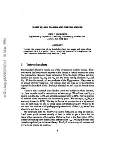
Fig. 4. ∆α/α and 1 σ errors from the many-multiplet method for three Keck/HIRES samples: Churchill (hollow circles), Prochaska & Wolfe (triangles), Sargent (squares). Upper panel: unbinned individual values. Middle panel: binned results for each sample. Lower panel: binned over the whole sample. To calculate the fractional look-back time we use H0 = 70 km s−1 Mpc−1 , Ωm = 0.3, ΩΛ = 0.7, implying an age of 13.47 Gyr. Table 1. Statistics for different samples. χ2ν is χ2 /(Nsys − 1) about the weighted mean Sample

Nsys

hzabs i

∆α/α (10−5 )

Churchill Prochaska & Wolfe Sargent Low-z (z < 1.8) High-z (z > 1.8) Raw total Fiduciala

27 38 78 77 66 143 143

1.00 2.27 1.76 1.07 2.55 1.75 1.75

−0.531 ± 0.223 −0.664 ± 0.219 −0.620 ± 0.129 −0.537 ± 0.124 −0.744 ± 0.167 −0.611 ± 0.100 −0.573 ± 0.113

a

χ2ν 1.109 2.024 1.182 1.064 1.739 1.373 1.023

Low-z sample + low-contrast sample + high-contrast sample with increased errors.

and the effect of removing individual transitions or entire ionic species from our fits. These are described in detail in [13,17]. Extra Scatter at High z Note that the scatter in the total low-z sample is consistent with that expected from the size of the error bars (i.e. χ2ν ≈ 1). However, at high-z, Fig. 4 shows

Constraining Variations in α, mq and ΛQCD

9

significant extra scatter. This is reflected in the high χ2ν values in Table 1. The weighted mean therefore exaggerates the true significance of ∆α/α at high-z. We have identified the major source of this extra scatter at high z. Consider fitting two transitions with very different line-strengths (e.g. Al ii λ1670 and Ni ii λ1709 in Fig. 3). Weak components near the high optical depth edges of the strong transition’s profile are not necessary to obtain a good fit to the data. Even though the vpfit χ2 minimization ensures that constraints on ∆α/α derive primarily from the optically thin velocity components, these weak components missing from the fit will cause small line shifts. The resulting shift in ∆α/α is random from component to component and from system to system: the effect of missing components will be to increase the random scatter in the individual ∆α/α values. This effect will be far larger in the high-z sample since only there do we fit transitions of such different line-strengths. We form a ‘high-contrast’ sample from the high-z (i.e. zabs > 1.8) sample by selecting systems in which we fit both strong and weak lines, i.e. any of the Al ii, Si ii or Fe ii transitions and any of the Cr ii, Ni ii or Zn ii ones. To obtain a more robust estimate of the significance of ∆α/α in this high-contrast sample, we have increased the individual 1 σ errors until χ2ν = 1 about the weighted mean. We achieve this by adding 1.75 × 10−5 in quadrature to the error bars of the 27 relevant systems. Other procedures for estimating the significance at high-z are discussed in [17]. Fig. 5 identifies the high-contrast sample and presents the binned results with increased error bars. Table 1 presents the relevant statistics. The above procedure results in our most robust estimate from the 143 absorption systems over the redshift range 0.2 < zabs < 4.2: ∆α/α = (−0.57 ± 0.11) × 10−5 . 2.4

Recent Criticisms of the MM Method

Bekenstein [25] has pointed out that the form of the Dirac Hamiltonian for the hydrogen atom changes in a theory where α is considered a dynamical field. He warns that the resulting shifts in energy levels could be important for the MM method. Reference [26] have extended Bekenstein’s model to many-electron atoms. They find that the energy shift within the Bekenstein model is proportional to ∆α/α defined in (2), up to corrections of order 1%. Thus, modifications to the energy shifts discussed by [25] for the hydrogen atom are not important for the MM method applied to many-electron metal ions. Bahcall et al. [27] criticized the MM method on many points, summarized in their table 3. Though none of these are real candidate explanations of our results, we address each criticism below to avoid future confusion: • Theory: Since one must calculate the q coefficients using sophisticated many-body techniques, [27] argue that the MM method is less reliable than, say, the AD method. The likely sources of error are discussed in detail by [20] and we give a flavour of them in Sect. 2.2. The q coefficients are known to high enough accuracy given our sample precision (discussed below). We again stress that if ∆α/α is really zero, one cannot manufacture a non-zero value through errors in the q coefficients (2) if systematic errors in the quasar spectra are not important.

10

M. T. Murphy, V. V. Flambaum et al.

Fig. 5. The fiducial sample. Low-z sample (triangles), low-contrast sample (squares) and high-contrast sample with increased error bars (circles). The weighted mean, ∆α/α = (−0.57 ± 0.11) × 10−5 , is our most robust estimate for the HIRES spectra

• Absolute or relative wavelengths?: Reference [27] argued that the MM method requires the measurement of absolute wavelengths in the quasar spectra1 . This is incorrect. Since we simultaneously determine the redshifts of the absorption components and ∆α/α (these are not degenerate parameters; Fig. 2) for each system, any velocity shift may be applied to the spectra and ∆α/α will be unaffected. A velocity-space shift is a systematic error for the absorption redshifts, not for ∆α/α. • Sample precision: It is trivial to estimate the expected precision available from our observational sample. We explained this calculation in [13] and repeat it here. The Keck/HIRES pixels cover ∼ 3 km s−1 and so one reasonably expects to centroid barely resolved features (with SN ∼ 30–50) to 0.3 km s−1 . One expects ∼ 4 features per absorption system to be well-centroided in this way, providing a velocity precision of ∆v ≈ 0.15 km s−1 or ∆ω ≈ 0.02 cm−1 for an ω0 ≈ 40000 cm−1 transition. The typical difference in q coefficient between the Mg i/ii and Fe ii lines is ∼ 1000 cm−1 and so, for a single Mg/Fe ii absorption system, (2) implies a precision of |∆α/α| ∼ 1 × 10−5 . With ∼ 50 such systems, one expects a precision |∆α/α| ∼ 0.14 × 10−5 (cf. Table 1). 1

This suggestion is present only in preprint versions 1 & 2 of [27] (astro-ph/0301507). It is removed from later versions. Despite this, we address this point here to avoid further confusion in the literature.

Constraining Variations in α, mq and ΛQCD

11

As shown in Fig. 2 (and figs. A.2 & A.3 in [24]), simulations also provide a simple “reality-check” on the sample precision. • Line misidentification and blending: Reference [27] argue we may have misidentified many absorption features. In high resolution (R ∼ 50000) spectra we largely resolve the velocity structure of absorption systems. Misidentifying transitions is highly improbable since, even by eye, the profiles of different species follow each other to within |∆v| < 1 km s−1 . Confirming this, we obtain good fits to the absorption profiles with the number of free parameters restricted by physical considerations (Sect. 2.3). Detecting blends from absorption at other redshifts is also greatly facilitated by high resolution. See [13,17] for thorough discussions of blending and Fig. 1 for an example. Even if we misidentified a small number of transitions in our sample and they miraculously mimicked the velocity structure of other detected transitions (thereby allowing a good fit), this would have a random, not systematic, effect on ∆α/α. Indeed, compared with the AD method, the MM method is distinctly robust against misidentifications and blends: many transitions constrain the velocity structure so identifying blends and misidentifications is all the more trivial. Also, any blends that are not identified have a smaller effect on ∆α/α since many other transitions contribute to the constraints. • Velocity structure: The MM method assumes that corresponding velocity components in different ions have the same redshift. Most transitions used are from ionic species with very similar ionization potentials and so absorption from these species arise should arise co-spatially. Consider a Mg ii velocity component blueshifted with respect to the corresponding Fe ii component by some kinematic effect in the absorption cloud. Clearly, this mimics ∆α/α < 0 for that component. However, kinematic effects would equally well redshift the Mg ii components. Thus, the effect on ∆α/α is random from component to component and absorption system to system. This argument is misunderstood in [27]: they feel it is unlikely that such random effects “average out to an accuracy of 0.2 km s−1 over a velocity range of more than 102 km s−1 ”, the latter quantity referring to the total velocity extent of a typical absorption system. Inspecting Fig. 4, it is clear that any extra scatter in ∆α/α from kinematic effects derives only from the gas properties on velocity scales less than typical b parameters, i.e. < 5 km s−1 . That we obtain excellent agreement between the velocity component redshifts in different species to a precision |∆v| ∼ 0.3 km s−1 illustrates this. If kinematic effects were important, they would be most prominent in the low-z values of ∆α/α from the Mg/Fe ii systems, appearing as an extra scatter beyond that expected from the 1 σ errors. This is not observed. We discuss kinematic effects in more detail in [28] and [17].

2.5

Isotopic Abundance Variations

As we discussed in [29,30] and emphasised in [17,31], the main possible systematic error for the low-z results is that relative isotopic abundances may differ

12

M. T. Murphy, V. V. Flambaum et al.

Fig. 6. (Left) Isotopic structures for relevant Mg/Si transitions from measurements [33,34,15] or calculations [32]. Zero velocity corresponds to the structure’s centre of gravity. (Right) Sensitivity of ∆α/α to isotopic abundance variations. We alter the heavy isotope abundances proportionately: the heavy element fraction for Mg is 25,26 ΓMg = const. × (0.10 + 0.11) where the numbers in parentheses are the terrestrial isotopic fractions of 25 Mg and 26 Mg. Much higher relative 25,26 Mg abundances in the absorbers can explain the low-z results but the high-z results (containing the Si ii systems shown) are insensitive to 29,30 Si abundances

between the absorption clouds and terrestrial environment/laboratory, as summarized in Fig. 6. The isotopic structures used for Mg transitions are discussed in [17] whereas those for Si are from calculations similar to [32]. To our knowledge, isotopic structures for the transitions of Fe ii are not known. However, these should be far more ‘compact’ than those of, say, Mg since the normal mass shift will be > 5 times smaller. The results in Figs. 4 & 5 were obtained by fitting the quasar spectra with terrestrial isotopic abundance ratios. For those systems where Mg lines and no Si lines are fitted, these results correspond to the large square on Fig. 6, vice versa for the large triangle. The Mg ii and Si ii systems approximately correspond to the low- and high-z samples respectively. If we change the heavy isotope abundances we note the marked change in ∆α/α for the Mg systems and the comparative insensitivity for the Si systems. This is expected given the distribution of q coefficients in Fig. 2 and the diversity of transitions fitted at high-z (see [17] for further discussion). In previous works we argued that the heavy isotope fraction for Mg in our absorbers is likely to be significantly less than the terrestrial value. This is based on observations of low metallicity2 , Z, stellar environments in our Galaxy [35,36] and theoretical models of Galactic chemical evolution [37,38] where significantly sub-solar heavy isotope fractions are observed/expected at the low Zs of our 2

Metallicity is the relative metal abundance with respect to that in the Solar System environment. For LSSs and DLAs, log10 Z typically ranges from −2.5 to −0.5.

Constraining Variations in α, mq and ΛQCD

13

absorption clouds. However, some stars in [35,36] and those in some globular clusters [39,40] are found to have super-solar values. At low Z, the heavy Mg isotopes are thought to be primarily produced by intermediate mass (IM; ∼ 2−8 M⊙ ) stars in their asymptotic giant branch (AGB) phase [41–43]. Reference [38] included a contribution from IM AGB stars in their chemical evolution model, finding sub-solar heavy Mg isotope abundances at low Z, consistent with the above observations. Recently, [44] noted that enhanced heavy Mg isotope abundances might be produced at low Z if one assumes an IM-enhanced stellar initial mass function (IMF) at high z. However, such an IMF seems incompatible with current constraints. See [45] for general discussion of the observational constraints on the IMF. More recently, [46] find Ar, S and O abundances consistent with a normal IMF in a high-z DLA. See also [47]. For example, an IM-enhanced IMF could produce vast amounts of Fe via type Ia supernovae [48], in disagreement with Galactic and DLA abundance studies. Moreover, AGB enrichment levels are constrained by the relative element abundances in the absorption clouds. For example, AGB stars produce large amounts of N relative to other enrichment processes (e.g. supernovae types Ia & II; e.g. [49]). However, the abundance of N relative to H is very low in DLAs, i.e. 10−3.8 –10−1.5 solar [50,51]. Overall, these points are a barrier to ad-hoc IMF changes such as those suggested by [44]. Though enhanced heavy Mg isotope fractions are a possible explanation of the low-z varying-α results, we again conclude that they are an unlikely one.

3 3.1

Varying α and mq /ΛQCD from Atomic Clocks Introduction

The hypothetical unification of all interactions implies that variation of the electromagnetic interaction constant α should be accompanied by variation of masses and the strong interaction constant. Specific predictions require a model. For example, the grand unification model discussed in [52] (see also [53,54]) predicts that the quantum chromodynamic (QCD) scale, ΛQCD , is modified as δα δΛQCD ≈ 34 . ΛQCD α

(3)

The variation of quark and electron masses in this model is given by δα δm ∼ 70 , m α

(4)

resulting in an estimate for the variation of the dimensionless ratio δα δ(m/ΛQCD ) ∼ 35 . (m/ΛQCD ) α

(5)

The large coefficients in these expressions are generic for grand unification models, in which modifications come from high energy scales: they appear because

14

M. T. Murphy, V. V. Flambaum et al.

the running strong coupling constant and Higgs constants (related to mass) run faster than α. This means that if these models are correct the variation of masses and strong interaction may be easier to detect than the variation of α. For the strong interaction there is generally no direct relation between the coupling constants and observable quantities, unlike the case for the electroweak forces. Since one can only measure variations in dimensionless quantities, we must extract from the measurements constraints on variation of mq /ΛQCD , a dimensionless ratio, where mq is the quark mass (with dependence on the normalization point removed). A number of limits on variation of mq /ΛQCD have been obtained recently from consideration of Big Bang Nucleosynthesis, quasar absorption spectra and the Oklo natural nuclear reactor which was active about 1.8 billion years ago [9,55–64]. Below we consider the limits which follow from laboratory atomic clock comparisons. Laboratory limits with a time base of several years are especially sensitive to oscillatory variation of fundamental constants. A number of relevant measurements have been performed already and many more have been started or planned. The increase in precision is very fast. 3.2

Nuclear Magnetic Moments, α and mq /ΛQCD

As pointed out by [65], measurements of the ratio of hyperfine structure intervals in different atoms are sensitive to variation of nuclear magnetic moments. The first rough estimates of the dependence of nuclear magnetic moments on mq /ΛQCD and limits on time variation of this ratio were obtained in [55]. Using H, Cs and Hg+ measurements [66], [55] limited the variation of mq /ΛQCD to about 5 × 10−13 yr−1 . Below we calculate the dependence of nuclear magnetic moments on mq /ΛQCD and obtain the limits from recent atomic clock experiments with hyperfine transitions in H, Rb, Cs, Hg+ and optical transitions in Hg+ . It is convenient to assume that the strong interaction scale ΛQCD does not vary, so we will speak about variation of masses. The hyperfine structure constant can be presented in the following form,      me me e 4  2 α Frel (Zα) µ . (6) A = const. × Mp ¯h2 The factor in the first bracket is an atomic unit of energy. The second, ‘electromagnetic’, bracket determines the dependence on α. An approximate expression for the relativistic correction factor (Casimir factor) for the s-wave electron is Frel =

3 , γ(4γ 2 − 1)

(7)

p where γ = 1 − (Zα)2 and Z is the nuclear charge. Variation of α leads to the following variation of Frel [66]: δα δFrel =K , Frel α

(8)

Constraining Variations in α, mq and ΛQCD

K=

(Zα)2 (12γ 2 − 1) . γ 2 (4γ 2 − 1)

15

(9)

More accurate numerical many-body calculations [18] of the dependence of the hyperfine structure on α have shown that the coefficient K is slightly larger than that given by this formula. For Cs (Z=55) K=0.83 (instead of 0.74), for Rb K=0.34 (instead of 0.29) and for Hg+ K=2.28 (instead of 2.18). The last bracket in (6) contains the dimensionless nuclear magnetic moment, µ, in nuclear magnetons (the nuclear magnetic moment M = µ × e¯h/2Mp c) and the electron–proton mass ratio, me /Mp . We may also include a small correction due to the finite nuclear size. However, its contribution is insignificant. Recent experiments measured time dependence of the ratios of hyperfine structure intervals of 199 Hg+ and H [66], 133 Cs and 87 Rb [67], and the ratio of the optical frequency in Hg+ and the 133 Cs hyperfine frequency [68]. In the ratio of two hyperfine structure constants for different atoms, time dependence may appear from the ratio of the factors Frel (depending on α) and the ratio of nuclear magnetic moments (depending on mq /ΛQCD ). Magnetic moments in a single-particle approximation (one unpaired nucleon) are: µ = [gs + (2j − 1)gl ] /2 for j = l + 1/2 and µ=

j [−gs + (2j + 3)gl ] 2(j + 1)

(10)

(11)

for j = l − 1/2. Here, the orbital g-factors are gl = 1 for valence protons and gl = 0 for valence neutrons. Present values of the spin g-factors, gs , are gp = 5.586 and gn = −3.826 for the proton and neutron. These depend on mq /ΛQCD . The light quark masses are only about 1% of the nucleon mass [mq = (mu + md )/2 ≈ 5 MeV]. The nucleon magnetic moment remains finite in the chiral limit of mu = md = 0. Therefore, one may think that the corrections to gs due to the finite quark masses are very small. However, there is a mechanism which enhances the quark mass contribution: π-meson loop corrections to the nucleon magnetic moments which are proportional to the π-meson mass mπ ∼ p mq ΛQCD . mπ =140 MeV is not so small. According to [69], the dependence of the nucleon g-factors on the π-meson mass can be approximated as g(mπ ) =

g(0) , 1 + amπ + bm2π

(12)

where a = 1.37 GeV−1 , b = 0.452 GeV−2 for the proton and a = 1.85 GeV−1 , b = 0.271 GeV−2 for the neutron. This leads to the following estimate: δgp δmπ δmq = −0.174 = −0.087 , gp mπ mq

(13)

δmπ δmq δgn = −0.213 = −0.107 . gn mπ mq

(14)

16

M. T. Murphy, V. V. Flambaum et al.

Equations (10,11,13,14) give variation of nuclear magnetic moments. For the hydrogen nucleus (proton) , δmq δgp δµ = −0.087 . = µ gp mq For

199

Hg we have the valence neutron (no orbital contribution), and so δmq δgn δµ = −0.107 . = µ gn mq

For

133

87

(16)

Cs we have the valence proton with j=7/2 and l=4, giving δµ δmq δmπ = 0.11 . = 0.22 µ mπ mq

For

(15)

(17)

Rb we have the valence proton with j=3/2 and l=1, resulting in δmq δmπ δµ = −0.064 . = −0.128 µ mπ mq

(18)

Deviation of the single-particle nuclear magnetic moment values from the measured values is about 30% and so we have attempted to refine them. If we neglect the spin-orbit interaction, the total spin of nucleons is conserved. The magnetic moment of the nucleus changes due to the spin-spin interaction because the valence proton transfers part of its spin, hsz i, to core neutrons (transfer of spin from the valence proton to core protons does not change the magnetic moment). In this approximation, gs = (1 − b)gp + bgn for the valence proton (or gs = (1 − b)gn + bgp for the valence neutron). We can use the coefficient b as a fitting parameter to reproduce nuclear magnetic moments exactly. The signs of gp and gn are opposite, therefore a small mixing, b ∼ 0.1, is enough to eliminate the deviation of the theoretical value from the experimental one. Note also that it follows from (13,14) that δgp /gp ≈ δgn /gn . This produces an additional suppression of the mixing’s effect, indicating that the actual accuracy of the single-particle approximation for the effect of the spin g-factor variation may be as good as 10%. Note, however, that we neglected variation of the mixing parameter b. This is difficult to estimate. 3.3

Results

We can now estimate the sensitivity of the ratio of the hyperfine transition frequencies to variations in mq /ΛQCD . For 199 Hg and hydrogen we have δα δ[mq /ΛQCD ] δ[A(Hg)/A(H)] = 2.3 − 0.02 . [A(Hg)/A(H)] α [mq /ΛQCD ]

(19)

Therefore, the measurement of the ratio of Hg and hydrogen hyperfine frequencies is practically insensitive to the variation of light quark masses and

Constraining Variations in α, mq and ΛQCD

17

the strong interaction. Measurements [66] constrain variations in the parameter α ˜ = α[mq /ΛQCD ]−0.01 : 1 d˜ α < 3.6 × 10−14 yr−1 . (20) α ˜ dt

Other ratios of hyperfine frequencies are more sensitive to mq /ΛQCD . For and 87 Rb we have δα δ[mq /ΛQCD ] δ[A(Cs)/A(Rb)] = 0.49 + 0.17 . [A(Cs)/A(Rb)] α [mq /ΛQCD ]

133

Cs

(21)

Therefore, measurements [67] constrain variations in the parameter X = α0.49 [mq /ΛQCD ]0.17 : 1 dX = (0.2 ± 7) × 10−16 yr−1 . (22) X dt Note that if the relation (5) is correct, variation of X would be dominated by variation of mq /ΛQCD : (5) would give X ∝ α7 . For 133 Cs and H we have δα δ[mq /ΛQCD ] δ[A(Cs)/A(H)] = 0.83 + 0.2 . [A(Cs)/A(H)] α [mq /ΛQCD ]

(23)

Therefore, measurements [70,71] constrain variations of the parameter XH = α0.83 [mq /ΛQCD ]0.2 : 1 dXH −14 yr−1 . (24) XH dt < 5.5 × 10 If we assume the relation (5), we would have XH ∝ α8 . The optical clock transition energy, E(Hg), at λ = 282 nm in the Hg+ ion, can be presented as   me e 4 Frel (Zα) . (25) E(Hg) = const. × ¯h2

Note that the atomic unit of energy (first bracket) is cancelled out and so we do not consider its variation. Numerical calculation of the relative variation of E(Hg) has given [18] δE(Hg) δα = −3.2 . (26) E(Hg) α Variation of the ratio of the Cs hyperfine splitting A(Cs) to this optical transition energy is equal to δα δ[me /ΛQCD ] δ[mq /ΛQCD ] δ[A(Cs)/E(Hg)] = 6.0 + + 0.11 . [A(Cs)/E(Hg)] α [me /ΛQCD ] [mq /ΛQCD ]

(27)

Here we have taken into account that the proton mass Mp ∝ ΛQCD . The factor 6.0 before δα appeared from α2 Frel in the Cs hyperfine constant (i.e. 2+0.83)

18

M. T. Murphy, V. V. Flambaum et al.

and α-dependence of E(Hg) (i.e. 3.2). Therefore, the results of [68] give the limit on variation of the parameter U = α6 [me /ΛQCD ][mq /ΛQCD ]0.1 : 1 dU −15 yr−1 . (28) U dt < 7 × 10

If we assume the relation (5), we would have U ∝ α45 . Note that we present such limits on |(dα/dt)/α| as illustrations only since they are strongly modeldependent.

4

Conclusions

We have presented evidence for a varying α based on many-multiplet measurements in 143 Keck/HIRES quasar absorption systems covering the redshift range 0.2 < zabs < 4.2: ∆α/α = (−0.57 ± 0.11) × 10−5 . Three independent observational samples give consistent results. Moreover, the low- and high-z samples are also consistent, which cannot be explained by simple systematic errors (Fig. 2). Our results therefore seem internally robust. The possibility that the isotopic abundances are very different in the absorption clouds and the laboratory is a potentially important systematic effect. A high heavy isotope fraction for Mg 25,26 25,26 (ΓMg ≈ 0.5) compared with the terrestrial value (ΓMg ≈ 0.21) may explain the low-z results (Fig. 6). However, observations of low-metallicity stars and 25,26 Galactic chemical evolution (GCE) models suggest sub-solar values of ΓMg in the quasar absorption systems. GCE models with a stellar initial mass function greatly enhanced at intermediate masses may produce large quantities of heavy Mg isotopes via asymptotic giant branch stars. However, such models disagree with the observed element abundances in quasar absorption systems. The highz results are insensitive to the isotopic fraction of 29,30 Si. However, we stress the need for theoretical calculations and laboratory measurements of isotopic structures for other elements/transitions observed in quasar absorption systems. Aside from a varying α, no explanation of our results currently exists which is consistent with the available observational evidence. The results can best be refuted with detailed many-multiplet analyses of quasar absorption spectra from different telescopes/instruments now available (e.g. VLT/UVES, Subaru/HDS). We have calculated the dependence of nuclear magnetic moments on quark masses. This leads to limits on possible variations in mq /ΛQCD from recent laboratory atomic clock experiments involving hyperfine transitions in H, Rb, Cs, Hg+ and an optical transition in Hg+ . These limits can be compared with limits on α-variation within the context of grand unification theories. Unfortunately, this comparison is strongly model-dependent. See, for example, [72].

References 1. J. Uzan: Rev. Mod. Phys. 75, 403 (2003) 2. C.J.A.P. Martins, ed.: Proc. JENAM2002: The cosmology of extra dimensions and varying fundamental constants (Kluwer, Netherlands, 2003)

Constraining Variations in α, mq and ΛQCD

19

3. S.S. Vogt et al.: ‘HIRES: The high-resolution echelle spectrometer on the Keck 10-m telescope’. In: Instrumentation in Astronomy VIII, ed. by D.L. Crawford, E.R. Craine (SPIE 2198, 1994) p. 362 4. P.J. Outram, F.H. Chaffee, R.F. Carswell: Mon. Not. Roy. Soc. 310, 289 (1999) 5. M.P. Savedoff: Nature 178, 689 (1956) 6. J.N. Bahcall, E.E. Salpeter: Astrophys. J. 142, 1677 (1965) 7. J.N. Bahcall: Astrophys. J. 149, L7 (1967) 8. A.M. Wolfe, R.L. Brown, M.S. Roberts: Phys. Rev. Lett. 37, 179 (1976) 9. L.L. Cowie, A. Songaila: Astrophys. J. 453, 596 (1995) 10. D.A. Varshalovich, V.E. Panchuk, A.V. Ivanchik: Astron. Lett. 22, 6 (1996) 11. V.A. Dzuba, V.V. Flambaum, J.K. Webb: Phys. Rev. Lett. 82, 888 (1999) 12. J.K. Webb, V.V. Flambaum, C.W. Churchill, M.J. Drinkwater, J.D. Barrow: Phys. Rev. Lett. 82, 884 (1999) 13. M.T. Murphy et al.: Mon. Not. Roy. Soc. 327, 1208 (2001) 14. U. Griesmann, R. Kling: Astrophys. J. 536, L113 (2000) 15. J.C. Pickering, A.P. Thorne, J.K. Webb: Mon. Not. Roy. Soc. 300, 131 (1998) 16. J.C. Pickering et al.: Mon. Not. Roy. Soc. 319, 163 (2000) 17. M.T. Murphy, J.K. Webb, V.V. Flambaum: Mon. Not. Roy. Soc. 345, 609 (2003) 18. V.A. Dzuba, V.V. Flambaum, J.K. Webb: Phys. Rev. A 59, 230 (1999) 19. V.A. Dzuba, V.V. Flambaum, M.T. Murphy, J.K. Webb: Phys. Rev. A 63, 42509 (2001) 20. V.A. Dzuba, V.V. Flambaum, M.G. Kozlov, M. Marchenko: Phys. Rev. A 66, 022501 (2002) 21. C.W. Churchill et al.: Astrophys. J. Supp. 130, 91 (2000) 22. J.X. Prochaska, A.M. Wolfe: Astrophys. J. Supp. 121, 369 (1999) 23. J.X. Prochaska et al.: Astrophys. J. Supp. 137, 21 (2001) 24. M.T. Murphy: Probing variations in the fundamental constants with quasar absorption lines. PhD thesis, University of New South Wales (2002). Available at http://www.ast.cam.ac.uk/∼mim 25. J.D. Bekenstein: Phys. Rev. Lett., submitted, preprint (astro-ph/0301566) (2003) 26. E.J. Angstmann, V.V. Flambaum, S.G. Karshenboim: in preparation 27. J.N. Bahcall, C.L. Steinhardt, D. Schlegel: Astrophys. J., accepted, preprint (astroph/0301507) (2003) 28. J.K. Webb, M.T. Murphy, V.V. Flambaum, S.J. Curran: Astrophys. Space Sci. 283, 565 (2003) 29. M.T. Murphy, J.K. Webb, V.V. Flambaum, C.W. Churchill, J.X. Prochaska: Mon. Not. Roy. Soc. 327, 1223 (2001) 30. J.K. Webb et al.: Phys. Rev. Lett. 87, 091301 (2001) 31. M.T. Murphy, J.K. Webb, V.V. Flambaum, S.J. Curran: Astrophys. Space Sci. 283, 577 (2003) 32. J.C. Berengut, V.A. Dzuba, V.V. Flambaum: Phys. Rev. A 68, 022502 (2003) 33. L. Hallstadius: Z. Phys. A 291, 203 (1979) 34. R.E. Drullinger, D.J. Wineland, J.C. Bergquist: Appl. Phys. 22, 365 (1980) 35. P.L. Gay, D.L. Lambert: Astrophys. J. 533, 260 (2000) 36. D. Yong, D.L. Lambert, I.I. Ivans: Astrophys. J., accepted, preprint (astroph/0309079) (2003) 37. F.X. Timmes, S.E. Woosley, T.A. Weaver: Astrophys. J. Supp. 98, 617 (1995) 38. Y. Fenner et al.: Publ. Astron. Soc. Australia 20, 340 (2003) 39. M.D. Shetrone: Astron. J. 112, 2639 (1996) 40. D. Yong, F. Grundahl, D.L. Lambert, P.E. Nissen, M.D. Shetrone: Astron. Astrophys. 402, 985 (2003)

20 41. 42. 43. 44. 45.

46. 47. 48. 49. 50. 51. 52. 53. 54. 55. 56. 57. 58. 59. 60. 61. 62. 63. 64. 65. 66. 67. 68. 69. 70.

71.

72.

M. T. Murphy, V. V. Flambaum et al. M. Forestini, C. Charbonnel: Astron. Astrophys. Supp. 123, 241 (1997) L. Siess, M. Livio, J. Lattanzio: Astrophys. J. 570, 329 (2002) A.I. Karakas, J.C. Lattanzio: Publ. Astron. Soc. Australia 20, 279 (2003) T. Ashenfelter, G.J. Mathews, K.A. Olive: Phys. Rev. Lett., submitted, preprint (astro-ph/0309197) (2003) R.C. Kennicutt Jr.: ‘Overview: The Initial Mass Function in Galaxies’. In: The Stellar Initial Mass Function (38th Herstmonceux Conference), ed. by G. Gilmore, D. Howell (Astron. Soc. Pac., San Francisco, CA, U.S.A, 1998) p. 1 P. Molaro, S.A. Levshakov, S. D’Odorico, P. Bonifacio, M. Centuri´ on: Astrophys. J. 549, 90 (2001) M. Pettini, C.C. Steidel, K.L. Adelberger, M. Dickinson, M. Giavalisco: Astrophys. J. 528, 96 (2000) K. Nomoto et al.: Nucl. Phys. A 621, 467 (1997) L.M. Dray, C.A. Tout, A.I. Karakas, J.C. Lattanzio: Mon. Not. Roy. Soc. 338, 973 (2003) M. Pettini, S.L. Ellison, J. Bergeron, P. Petitjean: Astron. Astrophys. 391, 21 (2002) M. Centuri´ on, P. Molaro, G. Vladilo, C. P´eroux, S.A. Levshakov, V. D’Odorico: Astron. Astrophys. 403, 55 (2003) P. Langacker, G. Segr`e, M.J. Strassler: Phys. Lett. B 528, 121 (2002) W.J. Marciano: Phys. Rev. Lett. 52, 489 (1984) X. Calmet, H. Fritzsch: Euro. Phys. J. C 24, 639 (2002) V.V. Flambaum, E.V. Shuryak: Phys. Rev. D 65, 103503 (2002) K.A. Olive, M. Pospelov: Phys. Rev. D 65, 085044 (2002) V.F. Dmitriev, V.V. Flambaum: Phys. Rev. D 67, 063513 (2003) V.V. Flambaum, E.V. Shuryak: Phys. Rev. D 67, 083507 (2003) M.T. Murphy, J.K. Webb, V.V. Flambaum, M.J. Drinkwater, F. Combes, T. Wiklind: Mon. Not. Roy. Soc. 327, 1244 (2001) A.I. Shlyakhter: Nature 264, 340 (1976) T. Damour, F. Dyson: Nucl. Phys. B 480, 37 (1996) Y. Fujii et al.: Nucl. Phys. B 573, 377 (2000) H. Oberhummer, A. Cs´ ot´ o, M. Fairbairn, H. Schlattl, M.M. Sharma: Nucl. Phys. A 719, 283 (2003) S.R. Beane, M.J. Savage: Nucl. Phys. A 713, 148 (2003) S.G. Karshenboim: Canadian J. Phys. 318, 680 (1997) J.D. Prestage, R.L. Tjoelker, L. Maleki: Phys. Rev. Lett. 74, 3511 (1995) H. Marion et al.: Phys. Rev. Lett. 90, 150801 (2003) S. Bize et al.: Phys. Rev. Lett. 90, 150802 (2003) D.B. Leinweber, D.H. Lu, A.W. Thomas: Phys. Rev. D 60, 034014 (1999) N.A. Demidov, E.M. Ezhov, B.A. Sakharov, B.A. Uljanov, A. Bauch, B. Fisher: ‘Investigations of the frequency instability of CH1-75 hydrogen masers’. In: Proc. of the 6th European Frequency and Time Forum, Noordwijk, Netherlands 1992. (European Space Agency, Noordwijk, 1993), p. 409 L.A. Breakiron: ‘A Comparative Study of Clock Rate and Drift Estimation’. In: Proc. of the 25th Annual Precise Time Interval Applications and Planning Meeting. (U.S. Naval Observatory Time Service Department, Washington DC, 1993) p. 401 T. Dent: Nucl. Phys. B, accepted, preprint (hep-ph/0305026) (2003)