Feb 13, 2015 - the bias we perform a Fisher matrix analysis and we adopt two different ..... In our analysis all three parameters b0, Q and A are free to vary in each redshift bin. ...... [34] D. J. Eisenstein, H.-J. Seo, and M. White, Astrophys.
Constraints on a scale-dependent bias from galaxy clustering L. Amendola1 , E. Menegoni2 , C. Di Porto3,6 , M. Corsi3 , E. Branchini3,4,5 1
arXiv:1502.03994v1 [astro-ph.CO] 13 Feb 2015
3
Institut F¨ ur Theoretische Physik, Ruprecht-Karls-Universit¨ at Heidelberg, Philosophenweg 16, 69120 Heidelberg, Germany 2 CNRS, Laboratoire Univers et Theories (LUTh), UMR 8102 CNRS, Observatoire de Paris, Universite’ Paris Diderot; 5 Place Jules Janssen, 92190 Meudon, France Dipartimento di Fisica "E. Amaldi", Universita’ degli Studi "Roma Tre", via della Vasca Navale 84, 00146, Roma, Italy 4 INFN, Sezione di Roma Tre, via della Vasca Navale 84, I-00146 Roma, Italy 5 INAF Osservatorio Astronomico di Roma, INAF, Osservatorio Astronomico di Roma, Monte Porzio Catone, Italy. and 6 INAF Osservatorio Astronomico di Bologna, via Ranzani 1, I-40127 Bologna, Italy We forecast the future constraints on scale-dependent parametrizations of galaxy bias and their impact on the estimate of cosmological parameters from the power spectrum of galaxies measured in a spectroscopic redshift survey. For the latter we assume a wide survey at relatively large redshifts, similar to the planned Euclid survey, as baseline for future experiments. To assess the impact of the bias we perform a Fisher matrix analysis and we adopt two different parametrizations of scaledependent bias. The fiducial models for galaxy bias are calibrated using a mock catalogs of Hα emitting galaxies mimicking the expected properties of the objects that will be targeted by the Euclid survey. In our analysis we have obtained two main results. First of all, allowing for a scale-dependent bias does not significantly increase the errors on the other cosmological parameters apart from the rms amplitude of density fluctuations, σ8 , and the growth index γ, whose uncertainties increase by a factor up to two, depending on the bias model adopted. Second, we find that the accuracy in the linear bias parameter b0 can be estimated to within 1-2% at various redshifts regardless of the fiducial model. The non-linear bias parameters have significantly large errors that depend on the model adopted. Despite of this, in the more realistic scenarios departures from the simple linear bias prescription can be detected with a ∼ 2 σ significance at each redshift explored.
I.
INTRODUCTION
In the next future large experiments like DESI [1] and Euclid [2] will use galaxy clustering to obtain simultaneous informations on the geometry of the Universe and the growth rate of density fluctuations by measuring the galaxy power spectrum or the two-point correlation function at different cosmic epochs. These studies will be based on large surveys of extragalactic objects and will allow to accurately estimate cosmological parameters, among which the contribution of the Dark Energy to the cosmic density, the nature of this elusive component and, finally, to test non-standard theories of gravity. Since one typically observes the spatial fluctuation in the galaxy distribution, not in the mass, some independent phenomenological or theoretical insight of the mapping from one to the other is mandatory. This mapping, which is commonly referred to as galaxy bias, parametrises our ignorance on the physics of galaxy formation and evolution and represents perhaps the most serious source of uncertainties in the study of the large scale structure of the Universe. Galaxy bias should not regarded as a simple “nuisance” parameter. Its estimate is not just necessary to obtain unbiased cosmological information. However, it also allows to discriminate among competing models of galaxy formation and the physical processes that regulate the evolution of stars and galaxies. Current limitations in the theoretical models of galaxy evolution do not allow to predict galaxy bias with an accuracy sufficient to constrain dark energy or modified gravity models [3]. The alternative approach is phenomenological: i.e. to estimate galaxy bias directly from the data. Ref. [4], among others, has shown that future galaxy redshift surveys contain enough informations to break the degeneracy between the galaxy bias, clustering amplitude and the growth factor, effectively allowing to estimate galaxy bias from the data itself. This come at the price of making some assumption on the biasing relation. In this work we assume then that the bias relation between the galaxy density field and the mass field is local, deterministic but not necessarily scale-independent. The hypotheses of a local and deterministic bias break down on galactic scales where stellar feedback processes and, more in general, baryon physics become important. These scales are small compared to the typical size of current and future galaxy surveys and can be effectively smoothed out by focusing on large scale clustering analyses. A scale-dependent and redshift-dependent bias is a well established observational fact. Its evidence has emerged from different type of clustering analyses ranging from 2-point statistics [5–15] higher order statistics[16–20], galaxy counts [21–23] and gravitational lensing [24–27]. In our analysis we therefore assume that galaxy bias is scale and redshift dependent. In doing so we shall adopt a parametric approach in which one assumes a priori a theoretically
2 justified analytic model for the scale dependent bias. In this approach we ignore a possible scale dependent bias deriving from primordial non-Gaussianity [28–30] whose signature, perhaps also detectable in next generation surveys [31], is however supposed to be seen on scales much larger than those relevant for galaxy bias. In this work we forecast the errors on cosmological and galaxy bias parameters and assess the robustness of our predictions against the choice of the bias and the fiducial model. More specifically, we consider two different parametrizations for the scale-dependent bias: a simple power-law model and the polynomial model proposed by [32]. Both provide a reasonable good fit to mock galaxies similar to those that will be targeted by Euclid. We also adopt two different fiducial bias models: a simple but rather unrealistic unbiased model, in which galaxies trace mass, and a more realistic model in which the bias parameters allow to match the 2-point clustering properties of the mock galaxies. Finally, we restrict the analysis to large scales to avoid strong non-linear effects, which allow us to consider linear prescriptions complemented by some additional term to account for mildly non-linearities. As dataset we assume a wide spectroscopic galaxy redshift survey spanning a large redshift range and consider, as a reference case, the upcoming Euclid survey [2]. The layout of the paper is as follows. In section II we provide the theoretical framework of our Fisher matrix analysis and discuss the bias models used. In section III we present the result of the analysis when galaxies are assumed to trace the underlying mass density field at all redshifts. In section IV we adopt a more realistic fiducial model for galaxy bias, calibrated using mock galaxy catalogs and repeat the analysis of the previous sections. The main results are summarised and briefly discussed in the last section. II.
THEORETICAL SETUP
Following [33] we model the observed galaxy power spectrum, Pobs at the generic redshift z as: � �2 2 DAf (z)H(z) f (z) 2 2 2 Pobs (z, k) = G (z)b (k, z) 1 + µ 2 (z)H (z) P0f (k) b(z, k) DA f +Pshot (z)
(1)
where DA is the angular-diameter distance, H(z) is the so called expansion history, i.e. the Hubble constant at redshift z, G(z) is the linear growth function normalized to unity at z = 0, f (z) = d log G/d log a is the growth rate, b(z, k) is the scale-dependent bias, P0 (k) is the matter power spectrum at the present epoch, µ is the cosine angle between the wavenumber vector ~k and the line of sight direction, Pshot is the Poisson shot noise contribution to the power spectrum and the subscript f identifies the fiducial model. We parametrize the growth rate as f = Ωγm with a constant growth index γ. We perform the forecast using the Fisher matrix information method, i.e. by approximating the likelihood as a Gaussian in the parameters around a particular fiducial model, i.e. a value of the parameters that is assumed to approximate the 2-point clustering properties of galaxies in the real Universe. Since we are mostly interested in constraining galaxy bias, we rounded off the values of the cosmological parameters of the fiducial model, rather than using latest experimental figures. We set h0 = 0.7, Ωm0 = 0.25; Ωb0 = 0.0445; Ωk0 = 0; primordial slope ns = 1; and the dark energy equation of state w0 = −0.95. Finally, we set γ = 0.545 and rms density fluctuation at 8 h−1 Mpc σ8 = 0.8. Errors in the measured spectrometric redshift, δz ≈ 0.001(1 + z), propagate into errors in the estimated distances, δz σr = H(z) . Under the hypothesis that they are independent on the local galaxy density we can model their effect on the estimated power spectrum as P (z, k) = Pobs (z, k) e−k
2
µ2 σr2
.
(2)
This term removes power on small scales and effectively damp nonlinear effects on wavenumber larger than σr−1 . In order to account for mildly nonlinear effects we follow [34, 35] and multiply the power spectrum by the damping factor ( " #) 2 2 2 2 µ Σ (1 − µ )Σ k ⊥ + . (3) exp −k 2 2 2 This elliptical Gaussian function models the displacement field in Lagrangian space on scales & 10 h−1 Mpc, where we focus our analysis. In this expression Σ⊥ and Σk represent the displacement across and along the line of sight, respectively. They are related to the growth factor G and to the growth rate f through Σ⊥ = Σ0 G and Σk = Σ0 G(1 + f ). The value of Σ0 is proportional to σ8 . For our fiducial cosmology where σ8 = 0.8 , we have Σ0 = 11 h−1 Mpc. This implies that power is removed below this scale.
3 Assuming that the fluctuation Fourier modes are Gaussian variates, the Fisher matrix at each redshift shell is [36, 37] ˆ kmax ∂ log P (kn ) ∂ log P (kn ) k2 Fij = 2π (4) · Vef f · 3 · dk ∂θi ∂θj 8π kmin where the derivatives are evaluated at the parameter values of the fiducial model. Here, the maximum frequency kmax (z) is set by the scale at which fluctuations grow nonlinearly while kmin (z) by the largest scale that can be observed in the given redshift shell. We set a hard small-scale cut-off kmax = 0.5 h−1 Mpc at all redshifts which, together with the damping terms (2) and (3) account for non linearities. On large scale we set kmin = 0.001 h−1 Mpc. However, its precise value is not very relevant since the contribution of low k modes to the Fisher matrix is negligible. Veff indicates the effective volume of the survey defined as: �2 � �2 ˆ � n (~r) P (k, µ) nP (k, µ) Veff ≡ d~r = Vsurvey (5) n (~r) P (k, µ) + 1 nP (k, µ) + 1 where n = n(z) is the galaxy density at redshift z. The second equality in Equation (5) holds if the co-moving number density is constant within the volume considered. This assumption, which we adopt in our analysis, is approximately true in a sufficiently narrow range of redshifts. For this reason, we perform the Fisher matrix analysis in different, non-overlapping redshift bins listed in Table I, together with their mean galaxy number density. The redshift range, the size of the bin and the number density of objects roughly match the analogous quantities that are expected in the Euclid spectroscopic survey. To improve the correspondency, we multiply the galaxy number densities in Table I by an "efficiency" factor 0.5 and assumes a survey area of 15,000 deg2 . For additional robustness of our results, we marginalize over the Alcock-Paczinsky parameters. That is, we convert the wavenumber norm k and direction cosine µ from the fiducial to the any other cosmology using a free Hubble function and angular diameter distance parameters and marginalize over them, instead of projecting over the background parameters Ωm0 , h0 . TABLE I: Redshift bins used in our analysis and their mean galaxy number density. Col. 1: central redshift of each redshift shell with width ∆z = 0.2. Col 2: Mean number density of objects in h3 Mpc−3 . These numbers match those expected for a Euclid-like survey according to [2]. z 0.6 0.8 1.0 1.2 1.4 1.6 1.8 2.0
A.
ndens 3.56 × 10⁻³ 2.42 × 10⁻³ 1.81 × 10⁻³ 1.44 × 10⁻³ 0.99 × 10⁻³ 0.55 × 10⁻³ 0.29 × 10⁻³ 0.15 × 10⁻³
Analytic models for scale-dependent bias
The final ingredient in Eq. (1) and the focus of this paper is the scale-dependent galaxy bias b(z, k). Several authors have proposed different models, both phenomenological and theoretical [32, 38–42]. In this work we are not too concerned on the accuracy of bias models. Our goal is to assess the impact of a scale-dependent galaxy bias in the analysis of future galaxy surveys. For this purpose we have decided to adopt two rather simple models, the Power Law and the Q-Model, that nonetheless provide a good match to the galaxy bias measured in numerical experiments, as we shall see. The reason for choosing these models is twofold. First, they have been already used in the literature, making it possible to compare our results with existing ones and use previous results to set the range in which the model parameters can vary. Second, their simple form allows us to compute the power spectrum derivatives in the Fisher matrix analytically. The Power Law bias model has the form [43]: � �n k b(z, k) = b0 (z) + b1 (z) , (6) k1
4 TABLE II: Bias parameters for Type 1 fiducial models. FM1-PL FM1-Q n=0 n=1 n=2 z all
b0 1
b0 b1 b0 b1 b0 Q A 1 0 1 0 1 0 0
where the pivot scale k1 is introduced only to deal with dimensionless parameters. Its value does not impact on our analysis and, without lack of generality, we set k1 = 1 h Mpc−1 . The slope n is not treated as a free parameter but is kept fixed. However, to check the sensitivity of our results on the power law index we have considered three different values: n = 1 , 1.28, 2. As we shall see the value n = 1.28 corresponds to the one that provides the best fit to the bias of mock galaxies measured in simulated catalogs. n = 1 also provides an acceptable fit to the mock galaxy bias. The case n = 2 should be regarded as an extreme case since it provides a poor fit to the simulated data both at large and at small scales. We note that the Power Law model is similar to the one proposed by [39] in those k−ranges in which the power spectrum can be approximated by a power law. The Q-Model is also phenomenological. It has been proposed by [32] from the analysis of mock halo and galaxy catalogs extracted from the Hubble volume simulation. Its form is � b(z, k) = b0 (z)
1 + Q(z)(k/k1 )2 1 + A(z)(k/k1 )
�1/2 ,
(7)
In our analysis all three parameters b0 , Q and A are free to vary in each redshift bin. Therefore, the Q-Model has additional degrees of freedom with respect to the Power Law model. Finally, we need to specify the parameters of the fiducial model. In this work we consider two different fiducial models, Type 1 and Type 2, corresponding to two different choices of parameters for each bias model, totalling to four fiducial models. Type 1 models (denoted as FM1-PL for the power law bias and FM1-Q for the Q-model) represent the simple but rather unphysical case of galaxy tracing mass at all redshifts. Let us stress that assuming a scale-independent fiducial model does not imply that we are assuming a scale-independent bias since we differentiate the power spectrum in the Fisher matrix with respect to the scale-dependent bias coefficients: b1 , Q, A. Instead, assuming a scale-independent fiducial model only implies that in Type 1 models the derivative is evaluated at the fiducial values b1 , Q and A = 0. The parameters that identify the fiducial models are listed in Table II. Note that we also consider for comparison the case of scale-independent bias (first row). This case is identical to choosing n = 0 in the power law model, i.e. to b(z) = b0 (z) + b1 (z), so we will refer to this case as n = 0 fiducial. Type 2 models (denoted as FM2-PL and FM2-Q) are more realistic. The fiducial parameters of the Power Law and Q-Models were determined by matching the bias of mock Hα emitting galaxies in the simulations described in Section IV A. Table III lists the parameters of the fiducial models. Note that for the power law cases the values of the parameters depend on the choice of the power law index n so that, since we explore the cases n = 1 , 1.28, 2, we end up by having several Power Law fiducial models. TABLE III: Bias parameters for Type 2 fiducial models.
z 0.8 1.0 1.2 1.4 1.6 1.8
n=1 b0 b 1 1.04 1.13 1.22 1.36 1.49 1.61
0.67 0.74 0.99 1.09 1.22 1.40
FM2-PL n = 1.28 b0 b1 1.09 1.19 1.30 1.44 1.58 1.72
0.66 0.75 0.97 1.06 1.19 1.40
FM2-Q n=2 b0 b1 1.17 1.28 1.41 1.55 1.71 1.88
0.68 0.79 1.02 1.12 1.25 1.44
b0
A
Q
1.26 1.36 1.49 1.63 1.75 1.92
1.7 1.7 1.7 1.7 1.7 1.7
4.54 4.92 5.50 5.70 6.62 6.99
The complete set of parameters that are free to vary is then h, Ωb0 , Ωm0 , Ωk0 , ns , γ, σ8 plus, for each redshift shell, the shot noise Pnoise and b0 , b1 or alternatively b0 , A, Q. This amounts to a total of 39 independent parameters when we adopt 8 redshift bins. All the other parameters (the bias power law index n, the damping model, the survey parameters like galaxy density, volume, redshift error as well as the dark energy parameters w0 and w1 are kept fixed).
5 B.
Derivatives in the Fisher Matrix analysis
In order to evaluate the Fisher matrix we compute the derivatives of the power spectrum in Eq.p (1) with respect to the parameters on the fiducial model. The 1σ error for each parameter of the model, pi , is σpi = (F −1 )ii , where F −1 is the inverse Fisher matrix. Focusing on the free parameters of the biasing function we have for the Power Law bias model: d ln P 2 2f µ2 |f = f − f f db0 b0 b0 (b0 + f µ2 ) 2f µ2 (k/k1 )n d ln P 2 |f = f (k/k1 )n − f f db1 b0 b0 (b0 + f µ2 )
(8) (9)
For the Q-model we have instead : 2f µ2 d ln P 2 � |f = f − � � �1/2 db0 1+Q (k/k )2 b0 + f µ2 bf0 bf0 1+Aff (k/k11 )
(10)
and d ln P f µ2 (k/k1 )2 (k/k1 )2 − |f = dQ 1 + Qf (k/k1 )2 1 + Qf (k/k1 )2 d ln P k/k1 |f = − + dA 1 + Af (k/k1 )
III.
1 f µ2 + bf0
h
1+Qf (k/k1 )2 1+Af (k/k1 )
i1/2
f µ2 (k/k1 )bf0 � i1/2 � h f 1+Qf (k/k1 )2 2 [1 + Af (k/k1 )] f µ + b0 1+Af (k/k1 )
(11)
(12)
TYPE 1 FIDUCIAL MODELS. RESULTS
In this Section we show the results of the Fisher Matrix analysis performed using Type 1 models FM1-PL and FM1-Q. They represent the case of a survey of objects that trace the underlying mass density field in an unbiased way.
A.
Power law case
For the power law model we have explored two cases corresponding to different choices of the power law index: n = 1 and n = 2. The more realistic case n = 1.28 will be considered in the next Section. In addition, we consider the case n = 0 that represents the scale-independent hypothesis often assumed in many Fisher matrix forecast papers. For this particular case we do not compute derivatives with respect to b1 . The parameters of the fiducial models are reported in Table II. The goal of our analysis is twofold: to assess the impact of a scale-dependent bias on the measurement of the cosmological parameters and to estimate the accuracy with which we can measure the parameters that characterise the bias. Let us first focus on the first task. The 1σ errors on the cosmological parameters are listed in Table IV. Unless otherwise specified, the quoted errors are always obtained after marginalising over all the other parameters. For all parameters except the mass variance σ8 and the growth index γ the errors are largely independent from n. In fact in most cases they slightly decrease when the scale dependence is stronger. The values of σ8 and γ show the opposite trend, although the effect is quite small (below 10 %). We conclude that allowing for a scale dependent bias has little effect on the precision in which we can measure most cosmological parameters. It is interesting to note that the accuracy of the growth rate γ is 4-5% when marginalising over all parameters, including the scale and redshift-dependent bias. Figure 1 gives a visual impression of this fact. It shows the 1-σ likelihood contours for σ8 and γ for most of the fiducial models explored in this paper. The likelihood ellipse obtained in the FM1-PL case when n = 1 (red, dotted curve) is only slightly larger than that corresponding to a scale-independent bias (continuous, black line). The likelihood contours obtained for n = 2, not plotted to avoid overcrowding, are also similar. We further notice that there is little correlation between σ8 and γ.
6
0.810
Σ8
0.805 0.800 0.795 0.790 0.50
0.55 Γ
0.60
FIG. 1: 68 % probability contours for σ8 and γ. Black, continuous: standard scale-independent case, i.e. n = 0. Red, Dotted: FM1-PL with n = 1. Cyan, continuous: FM1-Q. Blue, Dot-Dashed: FM2-PL with n = 1. Green, dashed: FM2-Q.
TABLE IV: 1σ errors on cosmological parameters for Type 1 fiducial models. Error σh σΩm σΩb σns σγ σσ8
n=0 0.036 0.015 0.0034 0.036 0.024 0.0036
FM1-PL n=1 n=2 0.038 0.037 0.016 0.015 0.0036 0.0034 0.042 0.036 0.025 0.028 0.0044 0.0045
FM1-Q 0.039 0.016 0.0036 0.044 0.029 0.0047
The expected 1σ errors for the bias parameters b0 and b1 are listed in Table V for the cases n = 0, 1 and 2. Errors on b1 are larger than those on b0 and their size increase with n. When n = 2 they are ten times larger than with n = 1. On the contrary, errors on b0 weakly depend on n. This is not surprising since b1 is constrained by the power spectrum behaviour at high k, the larger the value of n the larger the values of k, where our analysis is less sensitive due to the damping terms and the hard kmax cut. A second trend is with the redshifts: errors on the bias parameters increase with the redshift, irrespective of the n value. Again, this is not surprising since it merely reflects the fact that the effective volume of the survey monotonically decreases when moving to high redshifts due to the smaller galaxy densities. When compared to the results of Ref. [44], in which bias was assumed to be scale-independent, we notice that our constraints on b0 are twice weaker than their "optimistic, internal bias" case at z = 1.8 and z = 2.0. This quantifies the effect of allowing for an additional degree of freedom, the scale dependent bias, represented by the new parameter b1 . In Figure 2 we show the 68 % probability contours in the b0 -b1 plane for n = 1 and n = 2, respectively. Larger ellipses refer to higher redshift bins. For the case n = 1 there is a strong anti-correlation between b0 and b1 which stems from the fact that an increase in the linear bias term b0 can be partially compensated by reducing the amplitude of the scale-dependent term b1 . Increasing the scale dependency, i.e. setting n = 2 reduces the correlation between b0 and b1 . This is due to the fact that a strong scale dependent bias has little impact on large (k � k1 ) scales and therefore cannot effectively compensate a variation of the linear bias on the scales that are relevant for our analysis.
7 TABLE V: Errors on bias parameters for Type 1 fiducial models. FM1-PL n=0 n=1 n=2 z σb0 σb0 σb1 σb0 σb1 0.6 0.8 1.0 1.2 1.4 1.6 1.8 2.0
0.007 0.008 0.009 0.010 0.011 0.012 0.014 0.018
0.013 0.013 0.013 0.014 0.014 0.016 0.019 0.026
0.14 0.13 0.12 0.12 0.13 0.16 0.22 0.34
0.0081 0.0093 0.011 0.012 0.013 0.014 0.016 0.019
1.2 0.97 0.86 0.82 0.91 1.2 1.9 3.3
FM1-Q σb0
σQ
σA
0.017 0.017 0.017 0.018 0.019 0.023 0.027 0.037
3.04 2.5 2.2 2.2 2.5 3.4 5.4 9.4
0.35 0.32 0.31 0.31 0.34 0.42 0.59 0.97
4
b1
2
0
-2
-4
0.96
0.98
1.00 b0
1.02
1.04
FIG. 2: 68% probability contours for the parameters b0 and b1 of the FM1-PL model. The dotted red line is the case with n = 1 while the dashed line in blue shows the case n = 2. The redshift bins are z = 0.6, 1.8, 2.0, from inside out.
B.
Q-model
This version of Type 1 fiducial model is characterised by three parameters, b0 , A and Q, rather than two. We have repeated the same analysis performed as in the FM1-PL case and summarised the results in Tables IV and V. The errors on the cosmological parameters are very similar to those obtained in the FM1-PL case, confirming that the accuracy in the estimate of the cosmological parameters is little affected by the adoption of a scale-dependent bias model, even when we introduce an additional degree of freedom. For this reason the 68% error contours for σ8 and γ (cyan thick curve in Figure 1) are quite close to that of the FM1-PL n = 1 case (red, dotted curve). Errors on the linear bias parameters b0 (Table V) are small, with a magnitude similar to that of the FM1-PL case with n = 1. On the contrary, the errors on A and Q are quite large, although we cannot directly compare their size to the errors on b1 . This is not entirely surprising: it is the effect of having one more parameter to marginalize over. To further investigate the possible degeneracy among the bias parameters we plot the 68 % uncertainty contours in the A-Q plane in Fig. 3. The size of the errors, and consequently the area of the corresponding ellipse increases with the redshift. They are positively correlated and the strength of the correlation also increases with the redshift.
8 1.5
1.0
A
0.5
0.0
-0.5
-1.0
-1.5 -15
-10
-5
0 Q
5
10
15
FIG. 3: Contours plots for 68 % probability contours for the parameters A and Q of the FM1-Q model. We decided to plot only the bins z = 0.6, 0.8, 1.6, 1.8, 2.0, from inside out, to improve clarity.
IV.
TYPE 2 FIDUCIAL MODELS. RESULTS
In this Section we repeat the Fisher matrix analysis performed in the previous Section using the same models for the power spectrum but assuming a Type 2 fiducial model for the bias. The parameters of the fiducial models have been provided by the best fit to the bias of the simulated Hα galaxies that will be targeted by the Euclid spectroscopic redshift survey. According to Ref. [2] Euclid will produce a redshift catalog of Hα-line emitting galaxies with line flux above Hαmin = 3 · 10−16 erg cm−2 s−1 with high completeness and purity. Ideally, one would fix the parameters of the fiducial model by matching observations. Unfortunately, the samples currently available are too small to reliably estimate the bias of high redshift, Hα galaxies. For this reason we consider instead a catalog of simulated Hα galaxies designed to mimic the predicted properties of the objects that will be observed by Euclid and measure their bias from the clustering properties. The detailed procedure is described in the next Section. Another important difference with Section IV is that we now consider a smaller redshift range (z = [0.8, 1.8]). This is a conservative choice mainly driven by the goal of matching as close as possible the range that will be best exploited for scientific analyses in the Euclid survey.
A.
Galaxy bias from mock catalogs
We consider the so-called "100 deg2 light-cone" mock galaxy catalog [49] obtained by applying the semi-analytic galaxy formation model GALFORM [45] to the outputs of the Millennium N -body simulation [46]. The simulated volume consists of a light-cone with a sky coverage of 100.206 deg2 spanning the redshift range [0.0, 2.0]. Mock galaxies are characterised by angular position, redshift, co-moving distances and a number of observational properties among which the luminosity of the Hα line. From these mocks we selected a subsample of objects in the range z = [0.6, 2.0] and with Hα line flux larger than Hαmin . To estimate galaxy bias we have compared the power spectrum of the Hα galaxies to that of the linear mass power spectrum obtained from CAMB [47] in six redshift bin of width ∆z = 0.2. The galaxy bias and its dependence on k is obtained from the ratio of these two quantities. This bias estimate is quite noisy due to the limited number density of mock galaxies. To regularise its behaviour we fit the Power Law and Q-model and determine the parameters of the fiducial by minimising the χ2 difference between model and estimated bias. Dealing with analytic expression for the bias also facilitates its implementation in the Fisher matrix analysis. The detailed procedure to determine the realistic model the galaxy bias is as follows: • We extract six, partially overlapping cubic boxes from the simulated light cone. These boxes are fully contained in the light cone, aligned along the line of sight and centred at the redshifts indicated in Table III. Their size increases with the redshift.
9 • We select galaxies brighter than Hαmin in each box and compute a statistical weight to account for the selection implied by the flux cut. • We use a Fast Fourier Transform based estimator, similar to [48], to measure the power spectrum of the mock galaxies within each cube. We ignore the effect of peculiar velocities and limit our analysis between kmax = 1h Mpc−1 and kmin . The value of kmax is chosen to minimise the impact of shot noise and aliasing. The value of kmin depends on the redshift and is determined by the size of each box. • We estimate the scale dependent galaxy bias from the ratio between the mock galaxy power spectrum and the CAMB power spectrum of the mass obtained using the same cosmological parameters as the Millennium simulation. • We fit the power law model and the Q-model to the estimated mock galaxy bias, b(k, z), by minimising the χ2 of the residuals. In the procedure we assume that the errors on the estimated power spectrum are the same as of the power spectrum estimator computed in [48]. In the χ2 minimisation procedure we fixed some of the bias parameters. For the Power Law model we set n = 1, 1.28 and 2. For the Q-model we set A = 1.7 according to Ref. [32]. The minimisation is first carried out over a conservative range of wave numbers, [kmin , kmax ] = [0.03, 0.3], that is gradually increased in both direction and stop when χ2 /d.o.f. ∼ 1. Note that the value n = 1.28 is the one that provides the best fit to the measured bias when n is also free to vary. The parameters of the fiducial models obtained from the χ2 fit are listed in Tab. III. We reiterate that for the Power Law model the best fit to the data is obtained with n = 1.28. The quality of the fit is still acceptable for n = 1 whereas n = 2 provides a poor fit both at small and large k-values. For this reason the case n = 2 should be regarded as an extreme and somewhat unrealistic case.
B.
Power Law case
Table VI shows the 1σ errors on the cosmological parameters when one assumes FM2-PL as a fiducial model for galaxy bias. Errors are similar to those of the Type 1 model for all parameters except for σ8 and γ They show little or no dependence on the power law index n. Errors on σ8 and γ are significantly larger since these parameters are partially degenerate with the bias. Indeed, the amplitude of the power spectrum is sensitive to the combination σ8 b(k, z) and the strength of the redshift distortion to f /b(k, z). In addition σ8 and γ are significantly anti-correlated (solid ellipse in Fig. 1). This anti-correlation reflects the fact that an increase in amplitude of the mass power spectrum (i.e. an increase in σ8 ) can be compensated by a decrease in the growth rate Ωγm . The reason why this anti-correlation was not seen in the Type 1 model case is that in this new fiducial model the bias is significantly larger than unity. As a consequence a much larger increase in the growth rate is now required to compensate a variation in σ8 . TABLE VI: 1σ errors on cosmological parameters for Type 2 fiducial models. FM2-PL FM2-Q Error n = 1 n = 1.28 n = 2 σh σΩm σΩb σns σγ σσ8
0.035 0.035 0.029 0.031 0.015 0.014 0.012 0.013 0.0033 0.032 0.0028 0.0027 0.0402 0.038 0.029 0.034 0.036 0.035 0.036 0.052 0.0049 0.0048 0.0046 0.0073
The errors on the bias parameters b0 and b1 are listed in Table VII for the three power law indices considered. The trend with n is the same as in the Type 1 case. Errors on b0 do not significantly depend on n. They do increase with the redshift (although the relative error σb0 /b0 does not). Errors on b1 significantly increase with n. Fig. 4 illustrates the covariance between b0 and b1 . The different ellipses are centred at the best fit values b0 and b1 listed in Table III. As their magnitude steadily increases with the redshift the center of the corresponding ellipses shifts accordingly. Errors on b0 are small and show a weak dependence on the redshift and on n. Errors on b1 are comparatively larger, show a weak dependence on the redshift and a strong dependence on n. One consequence of this is that the possibility to detect a scale dependent bias depend on the bias model itself. For n = 1 the scale dependency, i.e. the
10 TABLE VII: Errors on bias parameters for Type 2 fiducial models.
z 0.8 1.0 1.2 1.4 1.6 1.8
FM2-PL n = 1.28 σb0 σb1
n=1 σb0 σb1 0.014 0.016 0.018 0.021 0.024 0.028
0.12 0.12 0.12 0.13 0.16 0.21
0.012 0.014 0.016 0.019 0.022 0.026
0.19 0.18 0.18 0.19 0.24 0.32
FM2-Q n=2 σb0 σb1 0.011 0.013 0.016 0.019 0.023 0.027
0.91 0.76 0.66 0.69 0.89 1.3
σb0 0.029 0.033 0.039 0.045 0.049 0.056
σQ σA 2.6 1.9 1.6 1.6 1.8 2.1
0.46 0.39 0.36 0.34 0.37 0.40
fact that b1 6= 0, is detected with a significance of more than 4σ in each redshift bin and to more that 3σ for n = 1.28, i.e. with the most realistic fiducial model. Instead, for the extreme case n = 2 the size of the errors hides the scale dependency of the bias.
C.
Q-model
For the FM2-Q case the errors on the cosmological parameters, listed in Table VI, are remarkably similar to those of the FM2-PL case except for σ8 and γ whose uncertainties are significantly larger. This is clearly illustrated by the 68% error ellipse in Fig. 1 (green, dashed curve) that also confirms the anti-correlation between the two parameters noticed in the Type 1 analysis. In addition, as in the Type 1 case, the increase in the error size reflects the fact that the number of free parameters in the Q-model is larger than in the Power Law model. The errors on b0 , A and Q are listed in the last three columns of Table VII. Relative errors on b0 are similar to those of the FM1-Q case and larger that those of the FM2-PL case, again reflecting the increase in the number of free parameter in the bias model. Absolute errors on A and Q are smaller than in the FM1-Q case and appear to be correlated, as shown in Figure 5, which is expected since the bias in the Q-model depends on their ratio (7). The errors on A, Q weakly depend on the redshift whereas the value of Q significantly increases both at small and at large redshift (the value of A is set equal to 1.7). What is most remarkable is the fact that in this realistic fiducial model the bias parameter Q is significantly (∼ 3σ) different from zero, meaning that the scale dependence in galaxy bias can be detected even adopting a 3-parameter model. For the parameter A this significance is smaller and depends on the redshift: it increases from ∼ 1σ at z = 0.8 to ∼ 2σ at z = 1.8.
V.
CONCLUSIONS
In this paper we have investigated the impact of a scale-dependent galaxy bias on the results of the clustering analysis performed in next generation surveys. We focused on the galaxy power spectrum and, as a case study, we have considered a spectroscopic redshift survey with characteristics similar to those expected for the Euclid survey. In particular we focused on two issues: i) the impact of a scale dependent bias on the estimate of the cosmological parameters and ii) the accuracy with which it will be possible to detect such scale dependence. For this purpose we have considered two different models for the scale-dependent galaxy bias and obtained a Fisher matrix forecast assuming two sets of fiducial models. Both scale dependent bias models are characterised by a linear bias parameter b0 and additional parameters that quantify scale dependence. However, in the Power Law model one of them, the power law index, is fixed, whereas in the Q model both parameters, A and Q, are free too vary. All bias parameters change with redshift, so they should really be regarded as functions specified at different redshifts. For as concerns the fiducial models, we have considered two scenarios. The first one is the simple but unrealistic case of a population of unbiased mass tracers. The second one is that of a more realistic galaxy bias relation calibrated on simulated catalogs of Hα-line emitting objects mimicking the expected characteristics of the Euclid survey. Our main results can be summarised as follows: • Allowing for a scale dependent bias does not increase significantly the errors on cosmological parameters, except for the growth index γ and the rms density fluctuation σ8 . More specifically, in our analysis we find that errors on h0 , Ωm0 , Ωb0 , Ωk0 , and ns are insensitive to a scale dependency in galaxy bias, to the specific form of scale-dependent bias and to the choice of the fiducial model.
11
3
2
2
b1
b1
3
1
1
0
0
-1
-1 1.0
1.2
1.4
1.6
1.8
2.0
1.0
1.2
1.4
1.6
1.8
2.0
b0
b0
3
b1
2
1
0
-1
1.0
1.2
1.4
1.6
1.8
2.0
b0 FIG. 4: 68 % probability contours for the parameters b0 and b1 of the FM2-PL model for different values of n. They are centred at the b0 and b1 values indicated in Tab. III. Ellipses of increasing redshifts are centred at increasing values of b0 . In the left upper panel we show the case n = 1. In the right panel we show the n = 1.28 case. In the low left panel we show the n = 2 case. Only the redshifts z = 0.8, 1.2, 1.6, 1.8 are shown to avoid overcrowding.
In fact these errors are only slightly larger than those expected when one assumes that bias is scale independent. On the contrary errors on γ and σ8 are rather sensitive to the bias model and to the fiducial. In the ideal scenario of a population of unbiased mass tracers the expected relative error on γ is smaller than 5 %. However, when a more realistic bias model and survey setup are adopted, the relative error increases to ∼ 6 % for a 2-parameter bias model and to ∼ 9 % for a 3-parameter model. Clearly, an accurate estimate of the growth index would benefit from a reliable model for galaxy bias that can be captured by few free parameters. In addition, γ and σ8 are correlated. This correlation is expected since the clustering analysis constrains the amplitude of the power spectrum, proportional to the product b(k, z)σ8 (z) and its redshift distortions, which are proportional to f (z)/b(k, z). The degree of degeneracy, however, depends on the fiducial, being larger when more realistic bias models are adopted. • The linear bias parameter b0 can be determined within a few %. The relative error is rather insensitive to the
12
2.0
1.5
A
1.0
0.5
0.0
-0.5
0
5 Q
10
15
FIG. 5: 68 % probability contours for the parameters A and Q of the FM2-Q model. We plot only the redshifts z = 0.8, 1.2, 1.6, 1.8, left to right, to avoid overlaps.
choice of the fiducial and slightly increases with the redshift. As expected, the errors increase with the number of free parameters in the model and therefore is larger in the Q Model than in the Power Law one. Yet, even in the worst case (the realistic case of a Type 2 Q-Model bias at z = 1.8) the relative error is of the order of 2 %. This is of the same order as the uncertainty in the estimate of b0 obtained when one assumes no scale dependency, i.e. when one does not consider derivatives with respect to bias parameters other than b0 in the Fisher matrix analysis (see e.g.[4]). • The accuracy with which one can estimate the bias parameters that describe the scale dependency depends on the bias model and on the fiducial. The case in which the scale dependence is stronger, i.e. the Power Law model with n = 2, provides the worst results. This is not surprising since in this case the scale dependence is pushed at small scales where our Fisher matrix analysis, optimised to probe linear to mildly nonlinear scales, is less sensitive. However, we should stress that this n = 2 case is hardly realistic. In fact this model provides a poor fit to the bias of Hα galaxies in the simulated Euclid catalog. On the contrary, the Q-model, the Power Law model with n = 1.28 and, to a lesser extent, the Power Law model with n = 1 match the bias estimated from the mocks. When we restrict our analysis to the more realistic cases we find that scale dependency can be clearly detected at all redshifts. The significance of the detection, quantified by the departures of the parameters b1 , A and Q from zero, depends on both the bias and the fiducial. For the Power Law model with n = 1 is larger than 4σ at each redshift, decreasing to ∼ 3σ for n = 1.28. For the Q-model scale dependence is best detected through the parameter Q (∼ 3σ) whereas the significance of a non zero A-value is expected to be smaller and redshift dependent. All in all we conclude that a significant detection of a scale dependent bias is within reach of next generation redshift surveys and that contemplating such scale dependence does not significantly decrease the accuracy in the estimate of most cosmological parameters. We note that a scale dependent bias can also be induced by primordial nonGaussianity. Its signature is expected on much larger scales than those affected by galaxy bias and there should be ample possibility to disentangle the two effects. Yet, the need to allow for additional free parameters to account for non-Gaussian features may have an impact on the precision of the analysis. We shall explore this issue in a future paper.
VI.
ACKNOWLEDGEMENTS
The research leading to these results has received funding from the European Research Council under the European Community’ s Seventh Framework Programme (F P 7/2007 − 2013 Grant Agreement no. 279954), therefore
13 EM acknowledges the financial support provided by the European Research Council. EB acknowledges the financial support provided by NFN-PD51 INDARK, MIUR PRIN 2011 ’The dark Universe and the cosmic evolution of baryons: from current surveys to Euclid’ and Agenzia Spaziale Italiana for financial support from the agreement ASI/INAF/I/023/12/0. LA acknowledges financial support provided by DFG TRR33 “The Dark Universe”. LA acknowledges useful discussions within the Euclid Theory Working Group. We wish to thank Alex Merson for providing the 100 deg2 Euclid light cone mock catalogs.
[1] D. Schlegel, F. Abdalla, T. Abraham, C. Ahn, C. Allende Prieto, J. Annis, E. Aubourg, and M. Azzaro, ArXiv e-prints (2011), 1106.1706. [2] R. Laureijs, J. Amiaux, S. Arduini, J. . Auguères, J. Brinchmann, R. Cole, M. Cropper, C. Dabin, L. Duvet, A. Ealet, et al., ArXiv e-prints (2011), 1110.3193. [3] S. Contreras, C. Baugh, P. Norberg, and N. Padilla, ArXiv e-prints (2013), 1301.3497. [4] C. Di Porto, L. Amendola, and E. Branchini, MNRAS 423, L97 (2012), 1201.2455. [5] P. Norberg, C. M. Baugh, E. Hawkins, S. Maddox, J. A. Peacock, S. Cole, C. S. Frenk, and J. Bland-Hawthorn, MNRAS 328, 64 (2001), arXiv:astro-ph/0105500. [6] P. Norberg, C. M. Baugh, E. Hawkins, S. Maddox, D. Madgwick, O. Lahav, S. Cole, C. S. Frenk, I. Baldry, J. BlandHawthorn, et al., MNRAS 332, 827 (2002), arXiv:astro-ph/0112043. [7] I. Zehavi, Z. Zheng, D. H. Weinberg, J. A. Frieman, A. A. Berlind, M. R. Blanton, R. Scoccimarro, R. K. Sheth, M. A. Strauss, I. Kayo, et al., Astrophys. J. 630, 1 (2005), arXiv:astro-ph/0408569. [8] A. L. Coil, J. A. Newman, M. C. Cooper, M. Davis, S. M. Faber, D. C. Koo, and C. N. A. Willmer, Astrophys. J. 644, 671 (2006), astro-ph/0512233. [9] S. Basilakos, M. Plionis, K. Kovač, and N. Voglis, MNRAS 378, 301 (2007), arXiv:astro-ph/0703713. [10] S. E. Nuza, A. G. Sanchez, F. Prada, A. Klypin, D. J. Schlegel, S. Gottloeber, A. D. Montero-Dorta, and M. Manera, ArXiv e-prints (2012), 1202.6057. [11] P. Arnalte-Mur, V. J. Martínez, P. Norberg, A. Fernández-Soto, B. Ascaso, A. I. Merson, J. A. L. Aguerri, F. J. Castander, L. Hurtado-Gil, C. López-Sanjuan, et al., ArXiv e-prints (2013), 1311.3280. [12] R. A. Skibba, M. S. M. Smith, A. L. Coil, J. Moustakas, J. Aird, M. R. Blanton, A. D. Bray, R. J. Cool, D. J. Eisenstein, A. J. Mendez, et al., ArXiv e-prints (2013), 1310.1093. [13] F. Marulli, M. Bolzonella, E. Branchini, I. Davidzon, S. de la Torre, B. R. Granett, L. Guzzo, and A. Iovino, ArXiv e-prints (2013), 1303.2633. [14] M. Tegmark and B. C. Bromley, ApJL 518, L69 (1999), astro-ph/9809324. [15] C. Di Porto, E. Branchini, J. Bel, F. Marulli, M. Bolzonella, O. Cucciati, S. de la Torre, B. R. Granett, L. Guzzo, C. Marinoni, et al., ArXiv e-prints (2014), 1406.6692. [16] L. Verde, A. F. Heavens, W. J. Percival, S. Matarrese, C. M. Baugh, J. Bland-Hawthorn, and T. Bridges, MNRAS 335, 432 (2002), arXiv:astro-ph/0112161. [17] E. Gaztañaga, P. Norberg, C. M. Baugh, and D. J. Croton, MNRAS 364, 620 (2005), arXiv:astro-ph/0506249. [18] I. Kayo, Y. Suto, R. C. Nichol, J. Pan, I. Szapudi, A. J. Connolly, J. Gardner, B. Jain, G. Kulkarni, T. Matsubara, et al., PASJ 56, 415 (2004), arXiv:astro-ph/0403638. [19] T. Nishimichi, I. Kayo, C. Hikage, K. Yahata, A. Taruya, Y. P. Jing, R. K. Sheth, and Y. Suto, PASJ 59, 93 (2007), arXiv:astro-ph/0609740. [20] M. E. C. Swanson, M. Tegmark, M. Blanton, and I. Zehavi, MNRAS 385, 1635 (2008), arXiv:astro-ph/0702584. [21] E. Branchini, ArXiv Astrophysics e-prints (2001), arXiv:astro-ph/0110611. [22] C. Marinoni, O. Le Fèvre, B. Meneux, A. Iovino, A. Pollo, O. Ilbert, G. Zamorani, L. Guzzo, and A. Mazure, A&A 442, 801 (2005), arXiv:astro-ph/0506561. [23] K. Kovač, C. Porciani, S. J. Lilly, C. Marinoni, L. Guzzo, O. Cucciati, G. Zamorani, A. Iovino, P. Oesch, M. Bolzonella, et al., Astrophys. J. 731, 102 (2011), 0910.0004. [24] H. Hoekstra, L. van Waerbeke, M. D. Gladders, Y. Mellier, and H. K. C. Yee, Astrophys. J. 577, 604 (2002), astroph/0206103. [25] P. Simon, M. Hetterscheidt, M. Schirmer, T. Erben, P. Schneider, C. Wolf, and K. Meisenheimer, A&A 461, 861 (2007), astro-ph/0606622. [26] E. Jullo, J. Rhodes, A. Kiessling, J. E. Taylor, R. Massey, J. Berge, C. Schimd, J.-P. Kneib, and N. Scoville, Astrophys. J. 750, 37 (2012), 1202.6491. [27] J. Comparat, E. Jullo, J.-P. Kneib, C. Schimd, H. Shan, T. Erben, O. Ilbert, J. Brownstein, A. Ealet, S. Escoffier, et al., MNRAS 433, 1146 (2013), 1302.5655. [28] N. Dalal, O. Doré, D. Huterer, and A. Shirokov, Phys. Rev. D 77, 123514 (2008), 0710.4560. [29] M. Grossi, L. Verde, C. Carbone, K. Dolag, E. Branchini, F. Iannuzzi, S. Matarrese, and L. Moscardini, MNRAS 398, 321 (2009), 0902.2013. [30] L. Amendola, S. Appleby, D. Bacon, T. Baker, M. Baldi, N. Bartolo, A. Blanchard, C. Bonvin, S. Borgani, E. Branchini, et al., Living Reviews in Relativity 16, 6 (2013), 1206.1225. [31] T. Giannantonio, C. Porciani, J. Carron, A. Amara, and A. Pillepich, MNRAS 422, 2854 (2012), 1109.0958.
14 [32] S. Cole, W. J. Percival, J. A. Peacock, P. Norberg, C. M. Baugh, C. S. Frenk, I. Baldry, J. Bland-Hawthorn, T. Bridges, R. Cannon, et al., MNRAS 362, 505 (2005), astro-ph/0501174. [33] H.-J. Seo and D. J. Eisenstein, Astrophys. J. 598, 720 (2003), astro-ph/0307460. [34] D. J. Eisenstein, H.-J. Seo, and M. White, Astrophys. J. 664, 660 (2007), astro-ph/0604361. [35] H.-J. Seo and D. J. Eisenstein, Astrophys. J. 665, 14 (2007), astro-ph/0701079. [36] D. J. Eisenstein, W. Hu, and M. Tegmark, ApJL 504, L57 (1998), astro-ph/9805239. [37] M. Tegmark, Physical Review Letters 79, 3806 (1997), astro-ph/9706198. [38] U. Seljak, MNRAS 325, 1359 (2001), astro-ph/0009016. [39] H.-J. Seo and D. J. Eisenstein, Astrophys. J. 633, 575 (2005), astro-ph/0507338. [40] A. E. Schulz and M. White, Astroparticle Physics 25, 172 (2006), astro-ph/0510100. [41] E. Huff, A. E. Schulz, M. White, D. J. Schlegel, and M. S. Warren, Astroparticle Physics 26, 351 (2007), astro-ph/0607061. [42] R. E. Smith, R. Scoccimarro, and R. K. Sheth, Phys. Rev. D 75, 063512 (2007), astro-ph/0609547. [43] J. N. Fry and E. Gaztanaga, Ap. J. 413, 447 (1993), astro-ph/9302009. [44] C. di Porto, L. Amendola, and E. Branchini, MNRAS 419, 985 (2012), 1101.2453. [45] R. G. Bower, A. J. Benson, R. Malbon, J. C. Helly, C. S. Frenk, C. M. Baugh, S. Cole, and C. G. Lacey, MNRAS 370, 645 (2006), astro-ph/0511338. [46] V. Springel, S. D. M. White, A. Jenkins, C. S. Frenk, N. Yoshida, L. Gao, J. Navarro, R. Thacker, D. Croton, J. Helly, et al., Nature (London) 435, 629 (2005), astro-ph/0504097. [47] A. Lewis, A. Challinor, and A. Lasenby, Astrophys. J. 538, 473 (2000), astro-ph/9911177. [48] H. A. Feldman, N. Kaiser, and J. A. Peacock, Astrophys. J. 426, 23 (1994), astro-ph/9304022. [49] The catalogs are publicly available at http://astro.dur.ac.uk/∼d40qra/lightcones/EUCLID/