Journal of Geophysical Research: Atmospheres RESEARCH ARTICLE 10.1002/2014JD022419 Key Points: • Water vapor maps from InSAR • Absolute water vapor maps by combining InSAR and GNSS • Geostatistical interpolation
Correspondence to: F. Alshawaf,
[email protected]
Citation: Alshawaf, F., S. Hinz, M. Mayer, and F. J. Meyer (2015), Constructing accurate maps of atmospheric water vapor by combining interferometric synthetic aperture radar and GNSS observations, J. Geophys. Res. Atmos., 120, 1391–1403, doi:10.1002/2014JD022419.
Received 8 AUG 2014 Accepted 8 JAN 2015 Accepted article online 10 JAN 2015 Published online 27 FEB 2015
Constructing accurate maps of atmospheric water vapor by combining interferometric synthetic aperture radar and GNSS observations Fadwa Alshawaf1,2 , Stefan Hinz1 , Michael Mayer2 , and Franz J. Meyer3 1 Institute of Photogrammetry and Remote Sensing, Karlsruhe Institute of Technology, Karlsruhe, Germany, 2 Geodetic
Institute, Karlsruhe Institute of Technology, Karlsruhe, Germany, 3 Geophysical Institute, University of Alaska Fairbanks, Fairbanks, Alaska, USA
Abstract Over the past 20 years, repeat-pass spaceborne interferometric synthetic aperture radar (InSAR) has been widely used as a geodetic technique to generate maps of the Earth’s topography and to measure the Earth’s surface deformation. In this paper, we present a new approach to exploit microwave data from InSAR, particularly Persistent Scatterer InSAR (PSI), and Global Navigation Satellite Systems (GNSS) to derive maps of the absolute water vapor content in the Earth’s atmosphere. Atmospheric water vapor results in a phase shift in the InSAR interferogram, which if successfully separated from other phase components provides valuable information about its distribution. PSI produces precipitable water vapor (PWV) difference maps of a high spatial density, which can be inverted using the least squares method to retrieve PWV maps at each SAR acquisition time. These maps do not contain the absolute (total) PWV along the signal path but only a part of it. The components eliminated by forming interferograms or phase filtering during PSI data processing are reconstructed using GNSS phase observations. The approach is applied to build maps of absolute PWV by combining data from InSAR and GNSS over the region of Upper Rhine Graben in Germany and France. For validation, we compared the derived PWV maps with PWV maps measured by the optical sensor MEdium-Resolution Imaging Spectrometer. The results show strong spatial correlation with values of uncertainty of less than 1.5 mm. Continuous grids of PWV are then produced by applying the kriging geostatistical interpolation technique that exploits the spatial correlations between the PWV observations.
1. Introduction Microwave signals propagating through the Earth’s atmosphere are affected by a time delay that increases or decreases according to the ionospheric and neutrospheric activities. For L-band signals, the ionosphere is a dispersive medium where a linear combination of multiple carrier frequencies can sufficiently reduce the ionospheric delay. In addition, for carrier frequencies in the C- or X-band ranges, the ionospheric effects are marginal [Gray et al., 2000; Meyer et al., 2006; Meyer, 2011]. The neutrosphere is, however, a nondispersive medium for frequencies below 30 GHz; therefore, the neutrospheric delay in satellite signals has to be determined and eliminated. The neutrospheric delay can be caused by dry gases, called dry delay, or by water vapor, called wet delay. Although the wet delay does not exceed 10% of the total neutrospheric delay, it is considered a significant source of variance in refractivity. This is because, in contrast to the dry delay, the wet delay has high temporal and spatial variations, and its value is not easily predictable. The time delay caused by water vapor has to be adequately reduced in the geodetic and remote sensing applications of the Global Navigation Satellite Systems (GNSS) and interferometric synthetic aperture radar (InSAR). For example, different approaches have been presented to reduce the neutrospheric effects in InSAR observations to provide maps of the surface deformation at a millimeter accuracy. These approaches are based on either temporal averaging [Hooper et al., 2007; González et al., 2010; Kampes, 2005] or calibration using external data [Li et al., 2006a; Onn and Zebker, 2006; Doin et al., 2009]. Numerical atmospheric models provide precipitable water vapor (PWV) maps that have also been exploited for correcting the neutrospheric phase distortions [Foster et al., 2006; Gong et al., 2010]. On the other hand, GNSS observations have been considered since the 1990s as an efficient tool for atmospheric sounding [Bevis et al., 1992; Rocken et al., 1995]. Since then, numerous methods used GNSS ALSHAFWAF ET AL.
©2015. American Geophysical Union. All Rights Reserved.
1391
Journal of Geophysical Research: Atmospheres
10.1002/2014JD022419
observations to produce estimates of the atmospheric water vapor, which are exploited to build water vapor maps [Luo et al., 2008; Jade and Vijayan, 2008; Karabati´c et al., 2011]. InSAR and GNSS signals are affected in a similar way by the atmosphere [Onn and Zebker, 2006]. Therefore, if the neutrospheric effect in the InSAR interferogram is successfully separated from other phase components, it can be investigated as a valuable source of information to determine the atmospheric water vapor content. Using InSAR observations as a meteorological tool is a relatively new research field. The focus of previous research was put on comparing the neutrospheric phase maps in InSAR with data from numerical atmospheric models, GNSS, and MEdium-Resolution Imaging Spectrometer (MERIS) to Figure 1. A SAR satellite acquires a region on the Earth, while signals anticipate the ability of these data to from the visible GNSS satellites (within the cone) are received by a GNSS mitigate phase distortions in InSAR antenna located within that region. images. Wadge et al. [2002] compared the PWV from InSAR, GNSS, and numerical atmospheric models. They observed a similarity in the model and satellite data, which can be useful for correcting the large horizontal gradients of water vapor in InSAR ground motion signals on mountains. Pichelli et al. [2010] have compared PWV difference maps from InSAR with corresponding maps from the mesoscale model (MM5). The results presented by the authors show good agreement between the InSAR and MM5 data. Therefore, they suggested an assimilation of the water vapor fields derived from InSAR with the model to improve the resolution and the structure of atmospheric patterns. Mateus et al. [2010] compared the PWV content estimated from GNSS observations with the PWV difference maps extracted from InSAR interferograms. The PWV estimates (temporal differences) from GNSS observations show similar values and similar spatial variations to those derived from InSAR. Also, the results presented by Meyer et al. [2008] show a good agreement between the PWV maps derived based on persistent scatterer InSAR (PSI) and corresponding maps from MERIS. GNSS data were used in previous studies [e.g., Onn and Zebker, 2006; Li et al., 2006b] to reduce the neutrospheric noise, particularly that caused by water vapor, from the InSAR interferograms. We, however, use GNSS together with InSAR to produce maps of the neutrospheric water vapor. There are intrinsic differences between the wet delay measurements from InSAR and GNSS. The SAR and GNSS satellites have different viewing geometries, as shown in Figure 1. While the right-looking SAR acquires an image at a swath width of about 100 km (for Envisat), a GNSS antenna receives the signals from all visible satellites up to a minimum elevation angle. The two systems also differ in the temporal and spatial density of the measurements. As shown in previous research and will be shown in this paper, PSI can produce wet delay maps at a high spatial resolution, whereas GNSS provide measurements at often widely separated individual sites. In contrast, the temporal resolution of the GNSS wet delay estimates, which can be 30 min or less, is significantly higher than that for PSI, which produces an image at a repeat cycle of several days. In addition, PSI produces maps of the wet delay difference between two acquisition times, while the method of precise point positioning is applied to estimate the total wet delay from the GNSS observations [Hobiger et al., 2008]. The wet delay maps of PSI are point observations; however, the wet delay measured at a GNSS antenna represents a spatial average corresponding to a conical section of the neutrosphere with a vertex at that antenna, as shown in Figure 1. ALSHAFWAF ET AL.
©2015. American Geophysical Union. All Rights Reserved.
1392
Journal of Geophysical Research: Atmospheres
10.1002/2014JD022419
Figure 2. (a) Study region in the Upper Rhine Graben in Germany and France. The red squares indicate the locations of the GNSS sites, while the black box defines the frame of the SAR image. (b) The temporal and perpendicular baselines of the 17 analyzed SAR images. (c) An interferogram corrected for the flat Earth and the topographic phase.
In this paper, we present a new method to combine the wet delay measurements, of complementary properties, from GNSS and PSI to build maps of the absolute PWV at the spatial density of the persistent scatterer (PS) points. Based on the temporal and spatial properties of atmospheric water vapor, we have to detect which water vapor components are derived from the PSI data and which might be eliminated by building the interferograms. Also, certain neutrospheric signals cannot be distinguished from other phase components (e.g., topography and orbital ramps) and might therefore be eliminated during InSAR data processing. We use GNSS PWV estimates to determine the missing PWV components at each PS point. This paper is organized as follows. The next section describes the study area and the data sets. Section 3 presents the strategy followed to derive wet delay maps from the InSAR interferograms. We also compare the results with the PWV maps measured by the sensor MERIS. In section 4, we present a new approach to combine the PWV data from GNSS and PSI to build absolute maps of water vapor at a high spatial density. Then, the ordinary kriging method is applied to produce regular grids of PWV. The last section presents a conclusion and discusses possible future improvements.
2. Study Area and Data Sets This study is carried out using data collected in the Upper Rhine Graben (URG) region in Germany and France as shown in Figure 2a. The InSAR interferograms are built from a stack of 17 coregistered Envisat SAR scenes. A SAR scene covers an area of 100 km × 100 km centered on 49◦ 09′ 38′′ N, 8◦ 04′ 45′′ E as shown by the black box in Figure 2a. The images are acquired in the time period of 2003 to 2008 during descending passes at time intervals of multiples of 35 days. The temporal and spatial baselines of the processed scenes are shown in Figure 2b. An interferogram formed from the images acquired on 29 November 2004 and 23 May 2005 is shown in Figure 2c. The URG region is well covered by permanent GNSS sites that provide data since 2002. We processed the observations from 10 GNSS sites located within or close to the SAR frame to estimate the absolute zenith wet delay (ZWD). In Figure 2a, the names are added to the GNSS sites that were operational within the period of SAR acquisitions. In addition, the URG region is geophysically very stable, showing little to no ALSHAFWAF ET AL.
©2015. American Geophysical Union. All Rights Reserved.
1393
Journal of Geophysical Research: Atmospheres
10.1002/2014JD022419
surface deformation at time scales of days to months [Fuhrmann et al., 2013]. This is relevant as it eases the process of neutrospheric phase extraction from the InSAR time series. The GNSS-based ZWD is estimated by processing observations from all visible GNSS satellites with elevations higher than the cutoff elevation angle (here 7◦ ). The estimated ZWD represents an average value over a conical section of the neutrosphere with a radius depending on the cutoff elevation angle; see Figure 1. Moreover, the estimated ZWD represents a temporal mean since we estimate one ZWD value using GNSS observations over a time window of an hour. This means that the spatial and temporal short-scale neutrospheric signals are not observed in the GNSS ZWD estimates. However, this is not limiting our approach, because the GNSS ZWD estimates are only used to model the elevation-dependent and long-scale wet delay signals, which have smooth and slow variations in space and time. Short-scale ZWD variations will be extracted from InSAR instead. The PWV maps derived by GNSS and PSI data combination are validated using PWV maps measured by MERIS. These maps are measured simultaneously with the SAR data, and they have a spatial resolution of 260 m × 290 m (full mode). MERIS data significantly underestimate the true values under cloudy weather conditions, since it measures the water vapor content only to the cloud top. Hence, only five cloud-free MERIS PWV maps are available for this study.
3. Wet Delay in InSAR Observations The interferometric phase for each pixel in the interferogram is a superposition of different contributions, i.e., 𝜙int = 𝜙topo + 𝜙disp + 𝜙neu + 𝜙iono + 𝜙orbit + 𝜙flat + 𝜙noise
(1)
where 𝜙topo is the topographic phase component; 𝜙disp is the phase component due to the Earth’s surface displacement between the two SAR acquisitions; 𝜙neu is defined as differential phase shift caused by the propagation of the signal through the neutrosphere; 𝜙iono is the differential phase shift due to the signal propagation through the ionosphere, which is negligible for C-band data; the phase component due to the inaccuracy of the satellite orbit is denoted by 𝜙orbit ; 𝜙flat corresponds to uncertainties in the Earth’s ellipsoidal reference surface; and 𝜙noise is the component due to the system thermal noise and the loss of coherence between the two acquisitions. The interesting term for this study is 𝜙neu , so all other terms have to be properly reduced. The interferograms are built with respect to a single reference image called the master, acquired on 29 November 2004 at 09:51 (UTC). A laser digital elevation model with a spatial resolution of 10 m × 10 m and 20 cm height accuracy is used to reduce the Earth’s reference and topographic phases from the interferograms. Then, PSI data processing was applied to the corrected interferograms to identify the stable point candidates. This is performed based on the Stanford Method for Persistent Scatterer [Hooper et al., 2007]. The PS candidates are selected in the first iteration such that the amplitude dispersion index is below a threshold value of 0.4. Then the phase measurements of these candidates are analyzed to reject partially stable (stable in some interferograms) or unstable points. The total number of PS points identified within the area of interest is 169,688, where the point density is high in urban regions and it is significantly lower in vegetated terrain, with an average density of 17 points/km2 . This density is, however, sufficient for atmospheric studies where we benefit from the spatial correlation of the atmospheric signal, as described in section 4. After the PS points are identified, a series of temporal and spatial filters are applied to extract the neutrospheric phase as described in Hooper et al. [2007]. Within the study area, only small long-term tectonic motions were observed [Fuhrmann et al., 2013]; therefore, we can assume the component 𝜙disp in (1) to be negligible. The neutrospheric path delay is related to the neutrospheric phase as follows: Δ𝜌psi =− s
𝜆 (𝜙 − 𝜙neu,m ) 4𝜋 neu,i
(2)
where 𝜙neu,m and 𝜙neu,i are the neutrospheric phase shifts at the master m and the ith (slave) acquisition times, respectively. The neutrospheric signal Δ𝜌psi s is the difference in the slant wet delay (SWD) plus some potential large-scale differences in the dry delay. The dry delay shows small variations over time for small temperature variations, and the remaining signal after interferogram formation has linear, long-wavelength ALSHAFWAF ET AL.
©2015. American Geophysical Union. All Rights Reserved.
1394
Journal of Geophysical Research: Atmospheres
10.1002/2014JD022419
spatial variations. Therefore, this component is eliminated when modeling and removing the orbital ramps [Zebker et al., 1997]. Hence, the delay extracted from the InSAR interferograms is the wet delay caused by water vapor. Since InSAR measures the difference between the neutrospheric path delay at two acquisition times, we need to reconstruct the path delay corresponding to each SAR acquisition time. There exist N − 1 neutrospheric delay-difference observations and N unknown neutrospheric delay values for each PS point, rendering the equation system underdetermined. To overcome this problem, it is necessary either to rely on external data or to define a constraint. It is challenging to have external data at the high resolution of the InSAR; hence, we chose a solution that is based on a least squares inversion (LSQ) concept that includes a conditioning constraint. To constrain the system, we assume that the mean of all SWD (here 17 samples) for each PS point approaches zero. This assumption intrinsically assumes that the differential neutrospheric delay can be considered a zero mean Gaussian process. Under these considerations, the linear model used to relate N − 1 observations (interferograms) to N unknowns (images) is ⎡ −1 0 … +1 0 … 0 ⎤ ⎡ psi ⎤ ⎡ ⎤ Δ𝜌psi ⎢ ⎥ ⎢ 𝛿𝜌s,1 ⎥ ⎢ s,1m ⎥ 0 −1 … +1 0 … 0 psi ⎢ ⎥ ⎢ 𝛿𝜌psi ⎥ ⎢ Δ𝜌s,2m ⎥ s,2 ⎢ ⋮ ⋮ ⋱ +1 ⋮ ⋱ ⋮ ⎥ ⎢ ⎥ ⋮ ⎢ 0 0 … +1 … −1 0 ⎥ ⎢ ⋮ ⎥⎥ = ⎢⎢ ⎥ ⎢ ⎥ ⎢ 𝛿𝜌psi ⎥ ⎢ Δ𝜌psi ⎥ s,(N−1)m ⎢ 0 0 … +1 0 … −1 ⎥ ⎢ s,N−1 ∑ psi N 1 psi ⎢ 1 1 … 1 … 1 1 ⎥ ⎣ 𝛿𝜌s,N ⎥⎦ ⎢⎣ i=1 N 𝛿𝜌s,i = 0 ⎥⎦ ⎣ ⎦ ⏟⏞⏞⏞⏞⏞⏞⏞⏞⏞⏞⏞⏞⏞⏞⏞⏞⏞⏞⏞⏞⏟⏞⏞⏞⏞⏞⏞⏞⏞⏞⏞⏞⏞⏞⏞⏞⏞⏞⏞⏞⏞⏟ ⏟⏞⏞⏟⏞⏞⏟ ⏟⏞⏞⏞⏞⏞⏞⏞⏞⏞⏞⏞⏟⏞⏞⏞⏞⏞⏞⏞⏞⏞⏞⏞⏟ B C A
(3)
A: Design matrix; size: N × N; N: number of SAR scenes. ); size: N × K ; K : is the number of PS points. B: Unknown partial neutrospheric delay values (𝛿𝜌psi s,i C: Contains N − 1 neutrospheric-difference observations (referred to the master m) for K PS points and the constraint (last row). The last entry of the matrix C defines the constraint that is added to overcome the rank deficiency of the system. The solution for (3) is found by applying the LSQ inversion, B = (A′ A)−1 A′ C
(4)
Each row of B contains the wet delay values for all PS points at a certain acquisition time. Since the temporally correlated neutrospheric signals are eliminated by forming the interferograms or when reducing certain phase components, the maps of the neutrospheric delay retrieved by the LSQ inversion contain only a part of the neutrospheric delay, which we call partial wet delay or partial PWV. In order to validate the partial wet delay maps derived from PSI, we have to find out which delay components may be extracted from the interferogram and which might be missing. Therefore, we analyzed maps of the absolute PWV measured by MERIS. We decomposed the PWV into a stratified (elevation-dependent) component, a turbulently mixed short-scale component, and a long-wavelength component. Figure 3 shows the three spatial PWV components, long wavelength, short wavelength, and elevation-dependent, for a MERIS PWV map. Depending on this decomposition, we should be able to define which components are present in the PSI data and which are missing. The elevation-dependent component is temporally correlated. Hence, it may be partially or totally eliminated by building interferograms or when reducing the topographic phase. This depends on the surface topography in the study area. In areas of strongly variable topography, it is very likely that an elevation-dependent wet delay signal will be observed in the interferogram [Onn and Zebker, 2006; Li et al., 2006b]. Our study region has a relatively flat topography; therefore, the elevation-dependent wet delay is eliminated in many interferograms. The long-wavelength PWV is not distinguished from the orbital ramps and hence is eliminated from the interferograms. The short wavelength wet delay component is temporally uncorrelated; therefore, it can be extracted from the interferograms. ALSHAFWAF ET AL.
©2015. American Geophysical Union. All Rights Reserved.
1395
Journal of Geophysical Research: Atmospheres
10.1002/2014JD022419
Figure 3. (a) Partial SWD maps derived from PSI and (b) the corresponding map from MERIS. Each pixel has the size of 300 m × 300 m.
We validate the wet delay maps derived from PSI using MERIS PWV maps. The PWV content in the vertical direction is related to the ZWD, 𝛿𝜌psi zw , with PWV = Π ⋅ 𝛿𝜌psi zw
(5)
where the constant of proportionality Π has an empirical value within the range 0.15–0.17 [Bevis et al., 1994]. In this work, we calculate Π using measurements of the air temperature collected at meteorological sites in the URG as described in Alshawaf [2013]. The SWD, 𝛿𝜌psi sw , can be mapped from the radar line of sight into the vertical direction using 𝛿𝜌psi = cos 𝜃inc ⋅ 𝛿𝜌psi zw sw
(6)
The simple mapping function cos 𝜃inc is sufficient for the SAR viewing geometry, where the angle 𝜃inc denotes the incidence angle of the radar. The value of 𝜃inc varies over the acquisition from near range to far range between 16.6◦ and 23.1◦ . We found that the accuracy of the wet delay is improved if the location and, hence, local look angle of every PS within the SAR satellite swath is considered when calculating the mapping function. Figure 4 shows maps of the partial wet delay from PSI and MERIS. The MERIS PWV is converted into ZWD using (5), and the SWD extracted from PSI is transformed to the zenith direction using (6). In order to perform a proper comparison, certain components have to be subtracted from the MERIS data. The first is the topography-dependent wet delay component, which is modeled by a linear regression with the known topographic height in the study area. The second component is a 2D linear trend estimated from the remaining signal, which represents the long-wavelength wet delay. For comparing the two data sets, PSI observations located within each MERIS cell are averaged. In regions where less than five PS points were observed, the MERIS cells are masked out. Finally, the partial wet delay maps from PSI and MERIS are compared. The maps in Figure 4 show a spatial correlation of 86% and an RMS value of 5.3 mm (0.85 mm PWV). On the basis of this analysis, we now reverse the process to reconstruct the components lost in the PSI observations using wet delay data from GNSS as presented in the next section. ALSHAFWAF ET AL.
©2015. American Geophysical Union. All Rights Reserved.
1396
Journal of Geophysical Research: Atmospheres
10.1002/2014JD022419
Figure 4. Components extracted from a MERIS PWV map.
4. Combining PSI and GNSS Wet Delay Observations According to the results presented in the previous section, the partial PWV maps derived from the PSI data often contain short-scale variations, while elevation-dependent and long-wavelength signals are missing. Accordingly, we use the GNSS-based PWV estimates to determine the elevation-dependent and the long-wavelength PWV components. We call the sum of both components the nonturbulent PWV. The strategy for estimating the PWV content from the GNSS observations was described in Alshawaf [2013], while in this section we present the method to extract the nonturbulent PWV based on the GNSS observations. This includes the elevation-dependent (vertically stratified) PWV and the long-wavelength signal of the PWV. It is worth mentioning that the missing PWV components need to be determined at each PS point, and estimating one set of parameters for the entire image is not sufficient. 4.1. Extracting Nonturbulent PWV From GNSS There are different models that relate the PWV to the Earth’s surface elevation. Davis et al. [1993] and Elosegui et al. [1998] described the dependence of the wet refractivity and hence the wet delay on the surface elevation by an exponential law, i.e., ZWDst = ZWD0 e−z∕H
(7)
where ZWDst is the vertically stratified wet delay, ZWD0 is the ZWD measured at the sea level, and H is the neutrospheric height where most water vapor resides (normally, 1–2 km). Onn and Zebker [2006] suggested a more general model, (8)
ZWDst (z) = C exp(−𝛼z) + z𝛼C exp(−𝛼z) + ΔLmin
where C , 𝛼 , and ΔLmin are the model parameters. By fitting the models in (7), (8), and linear regression to MERIS data, the model in (8) showed better fit to the PWV measurements at low altitudes where smooth and slow vertical variations are expected, according to relative humidity vertical profiles. After estimating the model parameters C , 𝛼 , and ΔLmin , the goodness of fit between the model and the observations is determined by calculating the reduced chi-squared statistic from the following formula [Onn and Zebker, 2006]: 2 𝜒gnss =
gnss 2 1 ∑ (ZWD (zi ) − ZWDst (zi )) 2 𝜈 i 𝜎gnss,wet
(9)
𝜈 is the degree of freedom, such that if there are 10 GNSS-based ZWD values and the model requires the estimation of three parameters, then we have seven degrees of freedom. The 𝜎gnss,wet is the GNSS-based ZWD estimation error of 5.048 mm, which is computed using MERIS observations as a reference due to the lack of a more accurate source of ground truth data. The goodness of fit might vary according to the sparseness of the GNSS sites and the neutrospheric state, as explained later. Also, when the ZWD is dominated by turbulence in the neutrosphere, the fitting might not converge, which requires removal of some measurements iteratively until convergence.
ALSHAFWAF ET AL.
©2015. American Geophysical Union. All Rights Reserved.
1397
Journal of Geophysical Research: Atmospheres
10.1002/2014JD022419
Figure 5. PWV from GNSS and the elevation-dependent model on (a) 5 September 2005 and (d) 23 April 2007 and the corresponding (b, e) elevation-dependent and (c, f ) long-wavelength PWV at the PS locations. For 23 April 2007: (g) PWV estimates at certain sites are removed; the corresponding (h) elevation-dependent and (i) long-wavelength components.
The GNSS sites are separated by distances greater than 20 km; therefore, local neutrospheric effects that are uncorrelated with the topography might be observed in some ZWDgnss estimates rather than the others. If the norm of the residuals after the fitting increases, it is then most likely that the differences contain a long-wavelength trend independent of the surface elevation. Therefore, we calculate the difference between the ZWDgnss estimates and the elevation-dependent model. Using the difference, we perform a linear regression by fitting the following model ΔZWD(x, y) = a𝜆 + b𝜙 + c
(10)
where 𝜆 and 𝜙 are respectively the longitude and latitude of the GNSS site, while a, b, and c are the linear model parameters. To retrieve the nonturbulent wet delay eliminated from the PSI data, we applied the above method using the wet delay estimates (converted into PWV) at 10 GNSS sites distributed within and close to the SAR frame (see Figure 2a). Since the GNSS data are used to model the PWV components with smooth spatial variations, it is not required to have a dense GNSS network, but the sites should be well distributed within the entire ALSHAFWAF ET AL.
©2015. American Geophysical Union. All Rights Reserved.
1398
Journal of Geophysical Research: Atmospheres
10.1002/2014JD022419
Table 1. Parameter Estimates and Goodness of Fit (𝜒 2 ) for the Elevation-Dependent ZWD From GNSS Observations at SAR Acquisition Timea Day 5 September 2005 23 April 2007 (1) 23 April 2007 (2)
C [mm]
𝛼 [km−1 ]
ΔLmin [mm]
𝜒2
3.37 3.34 3.25
6.78 0.0027 11.44
12.43 9.86 12.71
0.53 1.09 0.36
a (1) refers to the estimates using 10 GNSS sites, and (2) refers to the estimates using only four GNSS sites.
region covered by the SAR. First, we use the GNSS-based PWV values to estimate the parameters for the elevation-dependent model in (8). Figure 5a shows the elevation-dependent model estimated from GNSS observations on 5 September 2005 at the SAR overpass time. The estimated parameters C, 𝛼 , and ΔLmin are used to calculate the elevation-dependent PWV at each PS point, as shown in Figure 5b. Table 1 summarizes the estimated parameters and the goodness of fit. The norm of the residuals, and hence the goodness of fit, may increase or decrease depending on the activity of the neutrosphere at the SAR acquisition time and the sparseness of the GNSS sites. If the wet delay is dominated by the stratified wet delay, the goodness of fit will improve. However, if significant spatial variations due to the turbulent neutrosphere are observed, the fitting of the model in (8) will converge with a large value for 𝜒 2 . To estimate the long-wavelength component, the difference between the PWV values and the fitting in Figure 5a is calculated and the parameters of the model in (10) are estimated. These parameters are used to calculate the map in Figure 5c. The GNSS-based PWV observations on 5 September 2005 show significant spatial variations; therefore, fitting the model in (8) is achieved with a large 𝜒 2 value. In this case, the norm of the residuals is large and the magnitude of the long-wavelength signal is significant. This also holds for the other example on 23 April 2007; however, the fitting converged in this case to a nearly horizontal line (Figure 5d) with a significantly large 𝜒 2 value. Under certain weather conditions, the wet delay is dominated by the atmospheric turbulence or local advection effects; therefore, the model in (8) hardly converges, and the value of 𝜒 2 is significantly large. This is the case for 23 April 2007: the PWV map from MERIS demonstrates high spatial variations. It is observed that the PWV is high in the southern and northeastern parts of the area acquired by the SAR reflecting large local moisture advection compared to the other parts of the map (Figure 4b). The GNSS-based ZWD estimates also show higher PWV in the southern sites. Fitting the model (8) to the 10 GNSS observations results in a nearly horizontal line (Figure 5d), which means that the wet delay value remains unchanged for all points on the surface as shown in Figure 5e. The long-wavelength signal determined using the residuals is shown in Figure 5f. To improve the quality of the fitting, we iteratively removed Figure 6. The method used to derive the absolute PWV maps from GNSS GNSS-based PWV estimates that are dominated by local moisture advection and PSI data. ALSHAFWAF ET AL.
©2015. American Geophysical Union. All Rights Reserved.
1399
Journal of Geophysical Research: Atmospheres
10.1002/2014JD022419
Figure 7. Maps of the absolute PWV derived by combining GNSS and PSI observations on (a) 23 April 2007 and (c) 5 September 2005. The corresponding PWV maps from MERIS (b, d) .
until the 𝜒 2 value is minimized for the estimates in Figure 5g. The corresponding elevation-dependent and long-wavelength PWV are shown in Figures 5h and 5i, respectively. In Table 1, the second row (labeled (1)) presents the estimated parameters when using the PWV from the 10 GNSS sites. The third row (labeled (2)) contains the parameters estimated after removing the ZWD estimates below the red line in Figure 5d. The goodness of fit improved from 1.09 to 0.36, although the degree of freedom reduced to 1. 4.2. Absolute PWV Maps In order to build maps of the absolute water vapor, we combine the partial SWD maps derived from the interferograms with the nonturbulent (elevation-dependent and long-wavelength) SWD maps calculated based on ZWDgnss estimates. The steps required to build absolute PWV maps by combining GNSS and PSI data are summarized in the flowchart of Figure 6. We compared the maps of the absolute SWD with the PWV maps measured by MERIS. First, the SWD values were converted into the corresponding PWV using (5), and the results are then mapped into the zenith direction using (6). The results in Figure 7 show strong agreement between the PWV maps from MERIS and the GNSS and InSAR combination. Figure 7a shows the PWV map from MERIS on 23 April 2007 and the map derived by combining PSI and GNSS data (from the four sites in Figure 5g) against the corresponding maps from MERIS (Figure 7b). The maps show strong spatial correlation of 95% and an RMS value of 0.68 mm. If we use the GNSS data from the 10 sites in Figure 5d, the spatial correlation with MERIS is 94.1% and the RMS value is 0.84 mm. The PWV maps on 5 September 2005 in Figures 7c and 7d show spatial correlation of 87% and an RMS value of 0.88 mm. In this case, the MERIS PWV map shows higher values in the southwestern quadrant of the area. The lower values of PWV provided by the combination of PSI and GNSS might be due to the lack of GNSS sites in that quadrant, which ALSHAFWAF ET AL.
©2015. American Geophysical Union. All Rights Reserved.
1400
Journal of Geophysical Research: Atmospheres
10.1002/2014JD022419
Table 2. Spatial Correlation Coefficients (CC) Between PWV Maps From GNSS/InSAR Combination and MERIS at Five SAR Overpass Timesa Day
CC (%)
RMS (mm)
Mean (mm)
SD (mm)
75 87 80 79 95
1.00 0.88 0.76 1.50 0.68
0.07 0.15 -0.03 0.81 -0.43
1.00 0.86 0.75 1.34 0.65
27 June 2005 5 September 2005 17 July 2006 30 October 2006 23 April 2007 a The
RMS, mean, and the SD values of the difference maps are also given.
affects the estimation of the model parameters and increases the value of uncertainty. Table 2 summarizes the results for PWV maps at five different SAR acquisition times (where cloud-free MERIS data are available). The combination of PSI and GNSS provides PWV maps at the PS density. As observed from Figure 4, persistent scatterers are not detected in the regions of low coherence (e.g., forests and vegetation areas). In order to build regular grids of PWV, we apply the ordinary kriging approach that relies on the spatial correlation between the observations [Deutsch and Journel, 1998]. The PWV signal can be split into a long-wavelength signal modeled by a linear trend and another component that has short-scale variations. In order to apply the kriging method, first, the deterministic linear trend is estimated and subtracted from the observations, i.e., Z̃ = Z − T ⋅ 𝜷̂ , where Z is the vector of PWV observations and Z̃ contains the centered data (with zero mean). T is the design matrix for the input data such that each row of T has the entries longitude, latitude, and 1, and 𝜷̂ contains the estimated regression parameters. The signal Z̃ is used to estimate an experimental semivariogram 𝛾(h) as follows: 𝛾(h) =
|N(h)| ∑ 1 ̃ ui ) − Z( ̃ ui + h)]2 [Z( 2|N(h)| i=1
(11)
̃ ui ) is the observation (PWV here) at the location ui , and N(h) is the number of observation pairs separated Z( ̂ uo ) at the location uo is determined from by a displacement vector h. The kriging estimator Y( ̂ uo ) = To (uo ) ⋅ 𝜷̂ + k′ ⋅ Z̃ Y(
(12)
To is the design matrix for the output locations, and k contains the kriging weights [Cressie, 1993]. The ordinary kriging method was applied to the PWV maps derived from the combination of GNSS and PSI data on 23 April 2007. The experimental semivariogram and the semivariogram models, shown in Figure 8a, are determined assuming that the neutrospheric signal is spatially isotropic. The prediction map is shown in Figure 8b. The output map has a resolution of 1 km × 1 km, which requires block kriging [Cressie, 1990], as applied in Alshawaf [2013]. The RMSE values corresponding to the predictions are below 1.5 mm in most cases as shown in Figure 8c. The RMSE increases in areas of sparse observations (see Figures 7a and 8c).
Figure 8. (a) Experimental semivariogram and a spherical semivariogram model using the PWV map on 23 April 2007. The sill equals 139.76 mm2 , and the range is 44.1 km. (b) The PWV map at 1 km × 1 km derived by applying the ordinary kriging algorithm and (c) the RMSE values corresponding to the predictions.
ALSHAFWAF ET AL.
©2015. American Geophysical Union. All Rights Reserved.
1401
Journal of Geophysical Research: Atmospheres
10.1002/2014JD022419
5. Conclusions and Discussion We present a method for combining the wet delay derived from the PSI difference maps and GNSS sparse absolute estimates to build high-resolution maps of the total water vapor content in the neutrosphere. The neutrospheric wet delay map extracted from the interferograms has short-scale variations, while the long-scale and the elevation-dependent signals are reduced during PSI data processing. This is of course dependent on the surface elevation in the test site and the neutrospheric effects in the in the slave and master images. The test area of Upper Rhine in Germany has a smooth topography, and by a proper selection of the master image that has spatially smooth atmospheric variations, the extracted partial wet delay maps do not contain the elevation-dependent and long-wavelength wet delay components. These components are modeled using GNSS-based wet delay estimates and added to the partial wet delay maps extracted from the interferograms to derive absolute maps of the precipitable water vapor. By comparing the maps of the PWV measured by MERIS with those generated by applying our method, the results show strong spatial correlation with RMS values below 1.5 mm. We found that the quality of the derived PWV maps is improved by, first, calculating the value of the empirical constant Π in (5) using measurements of the surface temperature at the SAR acquisition time. Second, when mapping the PWV from the slant geometry of the radar to the zenith direction, it is required to consider the slight variations in the incidence angle over the whole image. Retrieving N partial wet delay maps from N − 1 wet delay-difference maps is not possible since the system is underdetermined. Therefore, to solve this system we add a constraint that restricts the temporal mean of PWV at each PS point to zero. This condition is fulfilled for a large image stack; however, the acquisitions available for this study are limited to 17. In this case, the LSQ solution is highly dependent of the master image. If the atmospheric signal in the master image has high spatial variations, the slave PWV maps will be affected by a random noise that differs for different master images. We found that this noise effect can be reduced, and the solution is stabilized if the selected master image has a spatially smooth wet delay signal. On the other hand, the LSQ solution is more reasonable for those slave images that have specific neutrospheric patterns with high spatial variations. An optimal selection of the master image is necessary, which requires information about the neutrospheric state from external sources. We compared the path delay observed in InSAR and GNSS not only in the zenith direction but also in the SAR line of sight. This provides accurate information about the neutrospheric signal observed in GNSS and InSAR data. In this study, elevation-dependent wet delay signals were not observed in the maps extracted from the interferograms. It may occur that the elevation-dependent wet delay component is only partially reduced, particularly in regions with steep surface topography. In this case, only the missing signal has to be reconstructed based on the GNSS data. It is important to mention that the challenge to separate the neutrospheric phase will increase in regions where surface deformations are observed. We described how ordinary kriging can be used to construct regular grids of PWV, filling areas of poor coherence. To overcome the drawback of high computational burden, we suggest replacing the ordinary kriging algorithm with the fixed-rank kriging method presented by Cressie and Johannesson [2008]. In addition, to improve the quality of PWV, especially in the regions of low coherence where the PSI data are missing, PWV data from other sources, for example numerical atmospheric prediction models, should be used. The approach for fusing multiple data sources should produce continuous grids of PWV with an improved quality at a low computational complexity. Acknowledgments The authors would like to thank the GNSS data providers: RENAG, RGP, Teria, and Orpheon (France), SAPOS®-Baden-Württemberg and Rheinland-Pfalz (Germany), European Permanent Network, and IGS. We thank the ESA for the SAR and MERIS data. We also thank the Landesanstalt für Umwelt, Messungen und Naturschutz Baden-Württemberg for providing the meteorological observations.
ALSHAFWAF ET AL.
References Alshawaf, F. (2013), Constructing water vapor maps by fusing InSAR, GNSS, and WRF data, PhD thesis, Karlsruhe Institute of Technology, Karlsruhe, Germany. Bevis, M., S. Businger, T. A. Herring, C. Rocken, R. A. Anthes, and R. H. Ware (1992), GPS meteorology: Remote sensing of atmospheric water vapor using the global positioning system, J. Geophys. Res., 97(D14), 15,787–15,801. Bevis, M., S. Businger, S. Chiswell, T. A. Herring, R. A. Anthes, C. Rocken, and R. H. Ware (1994), GPS meteorology: Mapping zenith wet delays onto precipitable water, J. Appl. Meteorol., 33(3), 379–386. Cressie, N. (1990), The origins of kriging, Math. Geol., 22(3), 239–252. Cressie, N. (1993), Statistics for Spatial Data, Wiley, New York. Cressie, N., and G. Johannesson (2008), Fixed rank kriging for very large spatial data sets, J. R. Stat. Soc., 70(1), 209–226. Davis, J. L., G. Elgered, A. E. Niell, and C. E. Kuehn (1993), Ground-based measurement of gradients in the “wet” radio refractivity of air, Radio Sci., 28(6), 1003–1018. Deutsch, C., and A. Journel (1998), GSLIB Geostatistical Software Library and User’s Guide.
©2015. American Geophysical Union. All Rights Reserved.
1402
Journal of Geophysical Research: Atmospheres
10.1002/2014JD022419
Doin, M.-P., C. Lasserre, G. Peltzer, O. Cavalié, and C. Doubre (2009), Corrections of stratified tropospheric delays in SAR interferometry: Validation with global atmospheric models, J. Appl. Geophys., 69(1), 35–50. Elosegui, P., A. Ruis, J. Davis, G. Ruffini, S. Keihm, B. Bürki, and L. Kruse (1998), An experiment for estimation of the spatial and temporal variations of water vapor using GPS data, Phys. Chem. Earth, 23(1), 125–130. Foster, J., B. Brooks, T. Cherubini, C. Shacat, S. Businger, and C. L. Werner (2006), Mitigating atmospheric noise for InSAR using a high resolution weather model, Geophys. Res. Lett., 33, L16304, doi:10.1029/2006GL026781. Fuhrmann, T., B. Heck, A. Knöpfler, F. Masson, M. Mayer, P. Ulrich, M. Westerhaus, and K. Zippelt (2013), Recent surface displacements in the Upper Rhine Graben—Preliminary results from geodetic networks, Tectonophysics, 602, 300–315. Gong, W., F. Meyer, P. Webley, D. Morton, and S. Liu (2010), Performance analysis of atmospheric correction in InSAR data based on the Weather Research and Forecasting Model (WRF), in IEEE International in Geoscience and Remote Sensing Symposium (IGARSS), pp. 2900–2903, IEEE, Honolulu, Hawaii. González, P. J., K. F. Tiampo, A. G. Camacho, and J. Fernández (2010), Shallow flank deformation at Cumbre Vieja volcano (Canary Islands): Implications on the stability of steep-sided volcano flanks at oceanic islands, Earth Planet. Sci. Lett., 297(3), 545–557. Gray, A. L., K. E. Mattar, and G. Sofko (2000), Influence of ionospheric electron density fluctuations on satellite radar interferometry, Geophys. Res. Lett., 27(10), 1451–1454. Hobiger, T., R. Ichikawa, T. Takasu, Y. Koyama, and T. Kondo (2008), Ray-traced troposphere slant delays for precise point positioning, Earth Planets Space, 60(5), e1–e4. Hooper, A., P. Segall, and H. Zebker (2007), Persistent scatterer interferometric synthetic aperture radar for crustal deformation analysis, with application to Volcán Alcedo, Galápagos, J. Geophys. Res., 112, B07407, doi:10.1029/2006JB004763. Jade, S., and M. Vijayan (2008), GPS-based atmospheric precipitable water vapor estimation using meteorological parameters interpolated from NCEP global reanalysis data, J. Geophys. Res., 113, D03106, doi:10.1029/2007JD008758. Kampes, B. M. (2005), Displacement parameter estimation using permanent scatterer interferometry, PhD thesis, Delft Univ. of Technol., Delft, Netherlands. Karabati´c, A., R. Weber, and T. Haiden (2011), Near real-time estimation of tropospheric water vapour content from ground based GNSS data and its potential contribution to weather now-casting in Austria, Adv. Space Res., 47(10), 1691–1703. Li, Z., J.-P. Muller, P. Cross, P. Albert, J. Fischer, and R. Bennartz (2006a), Assessment of the potential of MERIS near-infrared water vapour products to correct ASAR interferometric measurements, Int. J. Remote Sens., 27(2), 349–365. Li, Z., E. J. Fielding, P. Cross, and J.-P. Muller (2006b), Interferometric synthetic aperture radar atmospheric correction: GPS topography-dependent turbulence model, J. Geophys. Res., 111, B02404, doi:10.1029/2005JB003711. Luo, X., M. Mayer, and B. Heck (2008), Extended neutrospheric modelling for the GNSS-based determination of high-resolution atmospheric water vapor fields, Boletim de Ciencias Geodesicas, 14(2), 149–170. Mateus, P., G. Nico, R. Tomé, J. Catalão, and P. Miranda (2010), Comparison of precipitable water vapor (PWV) maps derived by GPS, SAR interferometry, and numerical forecasting models, Proc. of SPIE, 7827, 782814-1–782714-7, doi:10.1117/12.864733. Meyer, F. (2011), Performance requirements for ionospheric correction of low-frequency SAR data, IEEE Trans. Geosci. Remote Sens., 49(10), 3694–3702. Meyer, F., R. Bamler, N. Jakowski, and T. Fritz (2006), The potential of low-frequency sar systems for mapping ionospheric TEC distributions, IEEE Trans. Geosci. Remote Sens., 3(4), 560–564. Meyer, F., R. Bamler, R. Leinweber, and J. Fischer (2008), A comparative analysis of tropospheric water vapor measurements from MERIS and SAR, in IEEE International Geoscience and Remote Sensing Symposium (IGARSS), pp. IV-228–IV-231, IEEE, Boston, Mass. Onn, F., and H. A. Zebker (2006), Correction for interferometric synthetic aperture radar atmospheric phase artifacts using time series of zenith wet delay observations from a GPS network, J. Geophys. Res., 111, B09102, doi:10.1029/2005JB004012. Pichelli, E., R. Ferretti, D. Cimini, D. Perissin, M. Montopoli, F. S. Marzano, and N. Pierdicca (2010), Water vapor distribution at urban scale using high-resolution numerical weather model and spaceborne SAR interferometric data, Nat. Hazards Earth Syst. Sci., 10(1), 121–132. Rocken, C., T. V. Hove, J. Johnson, F. Solheim, R. Ware, M. Bevis, S. Chiswell, and S. Businger (1995), GPS/STORM-GPS sensing of atmospheric water vapor for meteorology, J. Atmos. Oceanic Technol., 12(3), 468–478. Wadge, G., et al. (2002), Atmospheric models, GPS and InSAR measurements of the tropospheric water vapour field over Mount Etna, Geophys. Res. Lett., 29(19), 1905, doi:10.1029/2002GL015159. Zebker, H. A., P. A. Rosen, and S. Hensley (1997), Atmospheric effects in interferometric synthetic aperture radar surface deformation and topographic maps, J. Geophys. Res., 102(B4), 7547–7563.
ALSHAFWAF ET AL.
©2015. American Geophysical Union. All Rights Reserved.
1403