Constructing Liberation Codes Using Latin Squares - CiteSeerX

Constructing Liberation Codes Using Latin Squares* Wang Gang, Liu Xiaoguang, Lin Sheng, Xie Guangjun, Liu Jing Department of Computer, College of Information Technology Science, Nankai University [email protected] Abstract1 In recent years, multi-erasure correcting coding systems have become more pervasive. RAID6 is an important 2-erasure correcting code specification. But there is no consensus on the best concrete RAID6 coding scheme. Plank developed a brand new class of RAID6 codes called the Liberation codes that achieves good encoding, updating and decoding performance. In this paper, we present a chained decoding algorithm for the Liberation codes. Its performance is comparable with the bit matrix scheduling algorithm developed by Plank, but is more intuitive and reveals the essence better. In the process, we present a new class of Liberation codes called the Latin Liberation codes. These codes are based on column-hamiltonian Latin squares, hence the name. They are superior to the Liberation codes in parameter flexibility and structure flexibility. Finally, we analyze the performance of several XOR-based RAID6 codes and give some suggestion on their application.

1. Introduction In recent years, as hard disks have grown greatly in size and storage systems have grown in size and complexity, it is more frequent that a failure of one disk occurs in tandem with unrecovered failures of other disks or latent failures of blocks on other disks. On a system using single-erasure correcting code such as RAID5, this combination of failures leads to a permanent data loss [1]. Hence, applications of multierasure correcting codes have become more pervasive. RAID6 is a 2-erasure correcting code specification [2]. Several concrete RAID6 schemes have been developed, and some are applied successfully. This paper presents *

This paper is supported partly by the National High Technology Research and Development Program of China (2008AA01Z401), NSFC of China (90612001), RFDP of China (20070055054), and Science and Technology Development Plan of Tianjin (08JCYBJC13000)

a chained decoding algorithm for the Liberation codes - an important RAID6 scheme. Constructing Liberation codes by Latin squares is also discussed in this paper. The outline of this paper is as follows. In Section 2 we discuss the known RAID6 codes. Section 3 is devoted to introducing some related combinatorics knowledge. In Section 4 we present the chained decoding algorithm, and the Latin Liberation codes are presented in Section 5. A theoretical analysis is discussed in Section 6. Conclusions and future works are presented in Section 7. stripe0 stripe1 stripe2 stripe3 stripe4 …

disk0 D D Q D P

disk1 D P D D Q

disk2 D Q D P D …

disk3 P D D Q D

disk4 Q D P D D

Figure 1. A typical RAID6 system.

2. Current RAID6 codes An erasure code for storage systems is a scheme that encodes the content on n data disks into m check disks so that the system is resilient to any t device failures [3]. Unfortunately, there is no consensus on the best coding technique for n, m, t > 1. RAID6 is a specification for m=t=2. A typical RAID6 system appears as depicted in Fig 1. Each disk is divided into fixed-size blocks (stripe units). All blocks with the same in-disk offset are organized into a stripe. Each stripe contains n data units and 2 check units P and Q. The identity of the data and check disks is rotated every stripe for small write load balance. A stripe is a self-contained 2-erasure correcting entity and the whole layout is just the cyclic repetition of a stripe, so we can focus only on single stripe when design a RAID6 code. Generally a RAID6 code should be a MDS code. The best known RAID6 codes are Reed-Solomon codes [4]. They are based on Galois Field, thus the computational complexity is a serious problem though

Figure 2. Current RAID6 codes and CHLS. optimized algorithms have been developed [5][6]. Fig 2.c shows the 6-disk RDP code. The standard Another category is so-called array codes that p+1-disk RDP code can be described by a (p-1)*(p+1) design a stripe as an array of data and parity symbols. code array. The disk P stores horizontal parity symbols In this paper, we focus on the horizontal codes, such as and the disk Q stores skew diagonal parity symbols, EVENODD [7], RDP [1] and Liberation [8]. too. RDP codes also can be constructed by clipped 2d“Horizontal” means that some disks contain nothing parity codes. Its strategy for the deleted Q parity but data symbols and the others contain only parity symbol is “parity dependent” - some P symbols have symbols. “Vertical” means that the data and parity the second role as a data member of some Q. symbols are stored together. Horizontal codes fit Fig 2.d shows the 7-disk Liberation code. It is also RAID6 specification well, but vertical codes don’t. So based on the 2d-parity code shown in Fig 2.a. A some important vertical codes, such as X-Code [9], Bstandard Liberation code can be described by a p*(p+2) Code [10], are not within the scope of this paper. code array. Unlike EVENODD and RDP, it adopts STAR Code [11] is a 3-erasure horizontal code, it boils “addition” instead of “deletion”. The original 2d-parity down to EVENODD when applied to RAID6 scenarios; code is well-preserved and some data symbols (Dijk) are arranged to participate in one extra Q group (Qk). Pyramid Code [12] is not MDS; WEAVER Codes [13] Plank’s construction method lets the ith symbol in the and HoVer Codes [14] are not MDS too and are not horizontal. So they are all out of our sight. jth disk participate in Pi and Q( i − j ) mod p . When j is odd, Fig 2.b shows the 7-disk EVENODD code. The p+ j the ( − 1)th data symbol is the “3-group” symbol standard EVENODD code with p+2 disks consists of a 2 (p-1)*p data array and a (p-1)*2 parity array. Note that p − j th the whole array instead of each row corresponds to a and its 2nd Q group is the ( ) Q group. When j is 2 stripe in Fig 1, and each column instead of each j symbol corresponds to a stripe unit. The “disk P” even (>0), the 3-group symbol is in row − 1 and it stores horizontal parity symbols and the “disk Q” 2 stores skew diagonal parity symbols. Dij denotes the j joins the ( p − )th Q group. data symbol that participates in Pi and Qj. Di* 2 participates in Pi and all Qs. Note that the parameter p must be a prime for Array codes can be regarded as layouts of binary EVENODD, RDP and Liberation. This leads to bad linear codes. For example, the symbols in the 7-disk parameter flexibility and implementation problems. EVENODD code are just the symbols (except P4, Q4 We have tried to generalize EVENODD and RDP and D40~D44) of the 35-disk 2d-parity code [15] shown using Latin squares [18][19]. In this paper, we apply in Fig 2.a (Di*=Di4). P4 and D40~D44 are deleted for 2this technique to the Liberation codes. erasure correcting. Q4 is deleted and the sum (over GF[2], namely XOR operation, the same hereinafter) S 3. Related combinatorics knowledge of its sons is added to every Q for MDS. Therefore, the computational performance is not optimal and each 3.1. Graph representation of 2-erasure codes column instead of each symbol must be implemented as a stripe unit to achieve optimal update penalty. Some literature refers to simple graph These properties are the inherent limitations of the representation of parity independent 2-erasure linear MDS horizontal codes [16][17].

Figure 3. Simple graph representation.

Figure 4. A P1F of K5,5.

codes in which each data symbol participates in exactly two parity groups [10][15][20]: let each vertex denote a parity symbol (group) and each edge denote a data symbol - the two endpoints of an edge are just the two parity symbols of the data symbol. So an array code can be described by a graph partition if the underlying linear code can be described by a simple graph. We have proven the following theorem [20]: Theorem 1. If an array code can be described by a partition of a simple graph, it is 2-erasure correcting iff the union of any pair of sub-graphs of the partition doesn’t contain the following two types of structures: 1. A path and its two endpoints. We call this kind of unrecoverable erasure Closed Parity Symbols Subset, CPSS for short. 2. A cycle. We call it CDSS - Closed Data Symbols Subset. Fig 3.a shows the graph that corresponds to a 15disk 2d-parity code. Fig 3.b shows an array code based on it. Fig 3.c gives a CPSS that corresponds to the unrecoverable 2-erasure (disk0, disk1), and Fig 3.d shows a CDSS that corresponds to the unrecoverable 2-erasure (disk2, disk3).

3.2. Perfect one-factorizations A one-factor of a graph G is a set of edges in which every vertex appears exactly once. A one-factorization of G is a partition of the edge-set of G into one-factors. A perfect one-factorization (P1F) is a one-factorization in which every pair of distinct one-factors forms a Hamiltonian cycle. There is a widely believed conjecture in graph theory: every complete graph with an even number of vertices has a P1F [21]. Fig 4 shows a P1F of K5,5.

3.3. Latin squares An n*n Latin square L is an n*n matrix of entries

chosen from some set of symbols of cardinality n, so that no symbol is duplicated within any row or any column. We select Ζn={0, 1, …, n-1} as the symbol set, it is also can be used as the row and column number set. The symbol in row r, column c of L is denoted by Lrc. A Latin square of order n can be described by a set of n2 triples of the form (row, column, symbol). Each row r of a Latin square L is the image of some permutation σr of Ζn, namely Lri=σr(i). Each pair of rows (r; s) defines a permutation by σr,s=σrσs-1. If σr,s consists of a single cycle for each pair of rows (r, s) in a Latin square L, we say L is row-hamiltonian. Similar concepts can be defined in terms of the column and symbol. In this paper, we are concerned with columnhamiltonian Latin squares, CHLS for short. Fig 2.e shows a CHLS of order 5, and σ1,4 of it. It is just the Cayley table C5 of the cyclic group of order 5. In fact, Cp is a CHLS when p is a prime number. There is a CHLS L of order n iff Kn.n=(V,W,E) has a P1F F={F0, …, Fn-1} [21]. To show this, we create three one-to-one correspondence: between the row set and V, between the symbol set and W, and between the column set and F. Namely, (i, j, k ) ( ∈ L) corresponds to the edge (vi, wk) in Fj. Obviously, the cycle pattern in σr,s in L corresponds to that in Fr ∪Fs. The P1F shown in Fig 4 corresponds to C5. There is another conclusion [21]: if Kn+1 has a P1F, then so does Kn,n. Thus we have a conjecture: Kn,n has a P1F (CHLS of order n exists) for n=2 and all odd positive integers n. Graph theorists have proven that all even(odd) numbers less than 54(53) are “Kn P1F numbers” (CHLS/Kn,n P1F numbers) and have found many larger Kn P1F numbers (CHLS/Kn,n P1F numbers).

4. The chained decoding algorithm An 2-erasure array code can be described by a partition, a P1F is just a partition, and there is a bijection between CHLS and P1F of Kn,n. Thus a

natural idea is constructing 2-erasure array codes by CHLS. In [18] and [19], we have tried this idea. Two algorithms are developed to construct EVENODD-like codes and RDP-like codes respectively by CHLS. We call the first kind of codes PIHLatin codes (Parity Independent Horizontal Latin codes), and the second kind PDHLatin codes (Parity Dependent Horizontal Latin codes). The key ideas of the two algorithms are similar: each column of the CHLS is used to construct a disk; one row is deleted to break the Hamiltonian cycles induced by disk pairs - CDSS are avoided; finally, parity symbols are arranged properly to avoid CPSS. Therefore, 2-erasure correcting is guaranteed. PIHLatin and PDHLatin are superior to EVENODD and RDP in parameter flexibility because the distribution of P1F numbers is far denser than that of prime numbers. Although horizontal shortening (deleting some data disks - assuming they contain nothing but zeros) can alleviate EVENODD and RDP’s problem, we have shown that it is harmful to encoding/decoding/updating performance [18][19]. The PIHLatin and PDHLatin codes constructed by C5 are respectively the 7-disk EVENODD code and the 6disk RDP code shown in Fig 2. In fact, PIHLatin and PDHLatin are the supersets of EVENODD and RDP respectively. We have shown that the relationship is proper superset [18][19]. Liberation codes can be described by Latin squares, too. Writing down the (first) Q index of every data symbol, we get a CHLS. For example, the 7-disk Liberation code shown in Fig 2.d corresponds to the CHLS shown in Fig 2.f. This CHLS is an isotopy of C5 (constructed by performing column swapping on C5). Examining Plank’s construction method [8], we can see that all “Liberation CHLS” are of this kind. The Q index matrix of a Liberation code is a complete CHLS. This means that any pair of disks induces a Hamiltonian cycle (CDSS). So how do Liberation codes tolerant all 2-erasures? The answer is the 3-group data symbols. Plank has proven that the Liberation codes are 2-erasure correcting by matrix description. He also presented a decoding algorithm named bit matrix scheduling algorithm [8]. But it’s hard to understand the interior mechanism through matrix description. There is a simple and intuitive decoding algorithm for PIHLatin and PDHLatin codes. Suppose that a 2-erasure (disk1, disk2) occurs in a 6disk RDP coding system. All horizontal parity groups and the 2nd and 3th skew diagonal parity groups lose exactly two symbols, we can’t recover them directly. But Q0 and Q1 lose only one symbol, we can start decoding from them. D01 can be reconstructed by summing all surviving symbols in Q1 first, then D02 is reconstructed using the horizontal parity group P0, then

D12 is reconstructed through Q2, and then D13 is recovered by P1, and so on, until D2 is recovered by P2. Similarly, D30 and D3 are reconstructed along another chain. Graph representation describes this algorithm visually. A reconstruction chain corresponds to an open path (the opposite of CPSS and CDSS) in the union of the failed disks (sub-graphs), and its starting point (D01, D30) corresponds to the end edge of the open path. Now we present a chained decoding algorithm for Liberation codes. We illustrate its correctness by several examples instead of a strict formal proof. The reconstruction of single-erasures is trivial, so we focus on four kinds of 2-erasures. The Two Parity Disks Fail In this case, decoding equals to encoding. The Disk Q and a Data Disk Fail Decodes the data disk using horizontal parity groups, and then encodes the Disk Q. The Disk P and a Data Disk Fail We can decode the data disk using Q parity groups. There is at most one 3-group data symbol in a data disk. Thus if the failed data disk contains a Dijk, we recover it through Qj first, and then recover Di’k through Qk (all other symbols in Qk including Dijk are prepared now). And then we can encode the disk P.

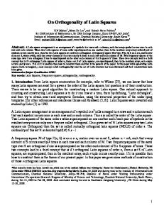
Figure 5. Chained decoding algorithm.

The First Data Disk and another Data Disk Fail The union of the two failed disks composes a cycle with a chord induced by the 3-group symbol. For example, Fig 5.a shows the sub-graph that corresponds to the 2-erasure (disk0, disk2) in a 7-disk Liberation coding system. The chord increases the degrees of v0 and w4 to 3. But v0 touches only 2 edges because the two dashed lines both denote D034. w4 touches really 3 edges. We call the former fake 3-vertex and the latter real 3-vertex. Examining the right sub-cycle, every involved parity groups (vertices) loses (touches) exactly 2 symbols (edges) except Q4 (w4) that loses 3 symbols: D14, D44 and D034. So, we can reconstruct the “tail” D14 by summing all surviving symbols in these

groups. This process can be described formally as i i is defined as the sum of the surviving follow. P i as the sum of the surviving symbols in Pi and Q i i ) also equals to the sum of the ii ( Q symbols in Qi. P i

lost symbols in the group. Huang et al gave them the name syndromes [11]. So we have: i = D ⊕D i0 = D ⊕ D Q i2 = D ⊕ D P P 034

00

0

00

20

i = D ⊕D i4 = D ⊕ D Q P 2 22 42 42 44 i = D ⊕D ⊕D Q 4 44 14 034 i i ⊕P i i i2 ⊕Q i4 ⊕Q ⇒ D = P0 ⊕ Q ⊕ P 14

0

2

20

22

(1)

Otherwise, the two tails point to each other inevitably. Thus the decoding process from any real 3-vertex must quit halfway at another real 3-vertex. We will show that Plank’s method guarantees this structure. i = D ⊕D i2 = D ⊕ D Q i0 = D ⊕ D P P 4 212 24 24 04 04 02 (2) i i i i i Q = D ⊕ D ⊕ D ⇒ D = P2 ⊕ Q ⊕ P0 ⊕ Q 2

02

212

We call this process cycle resolving and the traversal path resolving path. The dashed oval in Fig 5.a shows the resolving path described by formula 1. After the resolving process, we can recover all lost symbols clockwise from D14. A feasible resolving path should be a “Q shape” - a cycle with a tail edge. Moreover, it must pass one and only one real 3-vertex that is just the connection point between the cycle and the tail. This structure guarantees that all edges are touched precisely twice except the tail only once. Therefore summing all the syndromes decodes the tail symbol. In addition, chained decoding should be performed along the tail direction after cycle resolving. The decoding path must pass a fake 3-verrtex before pass its corresponding real 3-vertex. Otherwise, the decoding process will have to stop at the real 3-vertex. Thus, the left sub-cycle in Fig 5.a is also a feasible resolving path, but the decoding direction is anticlockwise. We can see that a resolving path always exists in this case, and chained decoding always complete. The syndromes seem to be calculated twice, one during cycle resolving and another during chained decoding. Therefore the decoding cost is far away from the optimal cost. But in fact, we can store the syndromes in the memory for the lost symbols once they are calculated during cycle resolving. Then they can be fetched and put into calculation immediately during chained decoding. Therefore, near-optimal performance is still guaranteed. Two Data Disks (Excluding the First Disk) Fail Fig 5.b shows the sub-graph that corresponds to the 2-erasure (disk1, disk3) in a 7-disk Liberation coding system. The dashed chord denotes the 3-group symbol D212 and the wavy chord denotes D145. The decoding process is similar to the last case. Formula 2 shows a resolving path that decodes D32. Another path decodes D212 as Formula 3 shows. Fig 5.b is the only recoverable structure. The real and fake 3-vertices must be interleaved on the cycle.

4

32

2

i = D ⊕D P i = D ⊕D i1 = D ⊕ D Q Q 0 3 301 10 10 13 13 43 i i P 4 = D43 ⊕ D41 Q1 = D41 ⊕ D301 ⊕ D212 i ⊕P i ⊕P i i1 ⊕ Q i4 ⊕Q ⇒ D =Q 212

4

32

0

3

(3)

1

Let a 2-erasure be described by an index pair (i, j ) (0 < i < j < p ) . All erasures can be divided into four classes by the parity of i and j. Because the code structure is symmetric, we can focus only on the erasures involving disk1 or/and disk2. Now we show that a 2-erasure (1, j) (j>1 is an odd number) leads to the recoverable structure. All operations are mod p arithmetic. An erasure (1, j) induces a Hamiltonian cycle v0-w-1-vd-wd-1-v2d-w2d-1-...w(p-1)d-1-vpd(v0) (d=j-1). The two fake 3-vertices are v p −1 and v p + j . The two real 3-vertices are w p −1 and 2

2

−1

2

2 p − j . We replace the two real 3-vertices with their 2

neighbors v p +1 and v p − j . This substitution doesn’t 2

2

+1

affect the relative order of the two kinds of vertices. We translate the original proposition into an equivalent problem: p is a prime; d is an even number between 2 and p-2; 0, d, …, (p-1)d is a permutation of p −1 p + d +1 {0, 1, …, p-1}; mark − 1 as red, and 2 2 p +1 p − d −1 and + 1 as black; then the red and and 2 2 black numbers are interleaved in the permutation. d d We shift the four numbers to 0, , 1 and 1 − . 2 2 This transformation doesn’t change the relative order of the vertices too. Suppose the indices of the four numbers in the permutation are x, y, u and v. Namely, d d x = 0, yd = mod p, ud = 1mod p, vd = (1 − ) mod p. 2 2 Thus 2 yd = d mod p . Since y and d are relative prime, p +1 . Note that we get 2 y = 1mod p . So we have y = 2 ( y + v − u )d = 0 mod p , thus y + v = u mod p . Thus p +1 y + v = u or y + v = u + p . Thus 0 < v < y ( = )