Constructing Transit Origin-Destination Matrices using Spatial Clustering
Ding Luo (corresponding author) Tel: +31 (0) 15 278 2762 Fax: +31 (0) 15 278 3179 E-mail:
[email protected] Oded Cats E-mail:
[email protected] Hans van Lint E-mail:
[email protected] Department of Transport & Planning Faculty of Civil Engineering and Geoscience Delft University of Technology Stevinweg 1, P.O. Box 5048, 2600 GA Delft, The Netherlands
Word count: 6273 words text + 6 figures x 250 words (each) = 7773 words
Resubmitted for possible publication in the Journal of Transportation Research Record.
Submission date: November, 2016
Luo, Cats & van Lint
2
ABSTRACT 1 2 3 4 5 6 7 8 9 10 11 12 13 14 15
So-called tap-in-tap-off smart card data have become increasingly available and popular as a result of the wide deployment of automatic fare collection systems for transit in many cities and areas worldwide. A new opportunity to obtain much more accurate transit demand than before has thus been opened to both researchers and practitioners. However, given that travelers in some cases are capable of choosing different origin and destination stations as well as different transit lines depending on their personal acceptable walking distance, aggregating the demand of spatially close stations becomes essential when constructing transit demand matrices. With an aim of investigating such problem using data-driven approaches, this paper proposes a k-means-based station aggregation method which can quantitatively determine the partitioning by considering both flow and spatial distance information. The method is applied to a case study of Haaglanden, The Netherlands, with a specified objective of maximizing the ratio of average intra-cluster flow to average inter-cluster flow while maintaining the spatial compactness of all clusters. With a range of clustering of different K performed first using the distance feature, a distance-based metric and a flow-based metric are then computed and ultimately combined together to determine the optimal number of clusters. The transit demand matrices constructed by implementing this method lay a foundation for further studies on shortterm transit demand prediction and demand assignment.
Luo, Cats & van Lint
1 2 3 4 5 6 7 8 9 10 11 12 13 14 15 16 17 18 19 20 21 22 23 24 25 26 27 28 29 30 31 32 33 34 35 36 37 38 39 40 41 42 43 44 45 46 47 48 49 50 51 52 53 54 55
1
3
INTRODUCTION
Transit demand studies and models form an essential part of any transit planning process. The purpose of such research is to estimate and evaluate passenger demand by using models and by collecting and analyzing data pertaining to current and future transit needs (1). Traditionally, the classical sequential four-step process has been extensively used in both academia and practice to estimate the aggregated travel demand for a number of traffic analysis zones (TAZ) which are predetermined based on geographical and socio-economic factors. Following this process, the share of transit demand is then computed at the step of modal split or mode choice using discrete choice models. This four-step method provides researchers and practitioners with a straightforward way to obtain transit demand when such demand could hardly be observed directly, though the results cannot always be desirably accurate. However, with the smart card automated fare collection (AFC) system being adopted by more and more transit agencies, a new type of data source is rapidly becoming available. AFC systems record individual travelers’ boarding and/or alighting information, greatly facilitating the research on passenger travel patterns that can support transit network planning, behavioral analysis and transit demand estimation and forecasting (2). A large amount of research efforts has been directed to transit origin-destination (O-D) estimation, especially for cases where only entry information or exit information is available, or even neither of them is available. Different methodologies have been proposed to infer O-D matrices for transit journeys with limited boarding or alighting information (3–10), and these methods can be categorized based on their estimation assumptions, including walking distances (buffer zones), transfer times, and last destination assumptions (11). Along with the increase in the number of methods, the importance of evaluation and validation on the O-D estimation methods and results has also been highlighted in a series of studies (12–16). Recently, Alsger et al. (11) used a high-quality dataset containing accurate boarding and alighting information to validate a multi-leg journey inference method, where the alighting information is assumed to be unknown for validation sake. The aforementioned O-D estimation studies focused on attaining more accurate journey inference, whereas less effort has been directed toward stop or station aggregation while constructing the demand matrices. Stop or station aggregation, in this context, means that transit users’ activities of originating from or destining to an individual stop can be virtually associated with an area which covers a number of adjacent transit stops or stations (17). In this sense, the demand at a more aggregate level can be of more practical use for both transit researchers and practitioners. McCord et al. (18) pointed out that the size of stop-to-stop O-D matrices makes it difficult to synthesize important flow patterns and to estimate stop-to-stop O-D passenger flows accurately. By grouping transit stops, however, the estimation, analysis, and communication of passenger flows can be improved. Furthermore, understanding the transit demand at an aggregate level was also motivated by Lee et al. (17) who highlighted that the ability to define a specific land-use type and the temporal characteristics related to passengers’ activities can be enhanced through the stop aggregation. In addition, the aggregation of stops is also in line with the analysis and modeling of transit users’ stop choice behavior which has been explored by several recent studies (19, 20). The rationale is that in reality, travelers are very often capable of choosing from a set of origin and destination stations which are within their acceptable distance. As a result of such behavior, different choices in transit services (modes and lines) can be characterized in terms of travel demand from one area to another. A limited number of studies involving the stop aggregation can be identified in the current literature. For instance, Chu and Chapleau (21) used the term “anchor points” to define the places that a person repeatedly visits, which usually include residence, work, or study locations. They performed spatial aggregation by grouping stops within 50 m of each other to form a new node. A so-called “stop-aggregation model” was later proposed by Lee et al. (22) and applied to studying the metro transit of the Minneapolis–Saint Paul metropolitan area in Minnesota (22, 23). This model aims to define a generalized definition of a “stop” that more closely matches the nature of locations serving as passenger origins and destinations. An aggregated area around a transit stop or station can thus be defined by three parameters: (a) distance or proximity, measured by using Euclidean and network distances in geographic information systems; (b) text in the description of the stop, queried using database tools in SQL; (c) the catchment area which is defined as how a stop relates to the land uses surrounding it. Alsger et al. (12) simply aggregated the estimated O-D trips according to the 1,515 zones in the Brisbane Strategic Transport Model to provide an overview of the results. McCord et al. (18) proposed two computationally efficient heuristic algorithms to aggregate bus stops at the route level in order to reduce the size of the O-D matrix for improved estimation, analysis, and communication. More recently, Tamblay et al. (24) developed a methodology to estimate zonal O-D matrix for a transit system. Based on a stop-to-stop O-D matrix created by using smart card data from Santiago de Chile, a Logit model was constructed to compute the probability that an observed trip using transit stops k and l (as their boarding and alighting points, respectively), was
Luo, Cats & van Lint
4
1 2 3 4 5 6 7 8 9 10 11 12 13 14 15 16 17 18 19 20 21 22 23 24 25 26 27 28 29 30 31 32 33 34 35 36 37 38
originated in zone i and ended in zone j. It is notable that in their methodology a zonal system must be pre-defined and a survey is required to help identify the model parameters.
39
2
40
2.1 Data overview
41 42 43 44 45 46 47
The smart card data set used in this study comes from Haaglanden, the conurbation surrounding The Hague in the Netherlands. It contains data collected from both buses and trams which are operated by HTM, the local transit operating company. As Figure 1 depicts, the transit network organized by HTM in this area consists of 12 tram and 8 bus lines serving 931 stations. For a more detailed description of the Dutch Smart Card System, the OV-Chipkaart, readers are referred to the study conducted by Van Oort et al. (27). Overall, the original transaction data are from March 2015 and contain 8,177,434 records (i.e. tap-in tap-out pair), covering a period of 31 days.
Unsupervised learning techniques have recently been employed to investigate spatial travel pattern and demand given their natural advantages in solving clustering problems (6, 25, 26). One of the successful applications turns out to be the identification of individual transit riders’ spatial and temporal travel patterns using the density-based spatial clustering of applications with noise (DBSCAN) algorithm (6, 25, 26). This specific algorithm stands out in its flexibility as it does not require predetermining the number of clusters, and identifies arbitrarily shaped clusters while implementing it. Ma et al. (6) first applied this algorithm to examine the spatial travel pattern of transit users in Beijing after inferring individuals’ journey chains. Adopting the approach proposed by Ma et al., Kieu et al. (26) later performed a two-level approach based on the standard DBSCAN algorithm to reveal both spatial and temporal travel patterns in South East Queensland, Australia. They further improved the efficiency of this approach by utilizing the existing knowledge of individual travel pattern while clustering the studied journey, developing a socalled Weighted-Stop DBSCAN (WS-DBSCAN) algorithm (25). The abovementioned studies highlight the importance of stop or station aggregation in analyzing AFC data. In many cases where transit services are well provided in both urban and suburban areas in terms of number of stations and lines (e.g., Haaglanden, the conurbation surrounding The Hague in the Netherlands, see Figure 1), the information of traveler O-D flow from one area to another, both of which contain a group of bus or tram stations, would be much better usable in transit modeling, prediction and management than by examining them at individual stop level. This paper proposes a k-means-based station aggregation methodology which can in four steps quantitatively determine the clustering by considering both flow and spatial distance information. This method is applied to a case study of Haaglanden, The Netherlands, by specifying a criterion that the ratio of average intra-cluster flow to average intercluster flow should be maximized while maintaining the spatial compactness of all clusters. In the first step, we obtain a number of different clustering scenarios by implementing the standard k-means algorithm with the geodesic distance considered as the only feature. Then, two metrics based on spatial distance and passenger flow respectively are computed, and finally integrated to determine the optimal number of clusters. The proposed data-driven method allows us to obtain clusters that are on one hand sufficiently large to enable the consideration and modeling of travel alternatives between parts of the network, while on the other hand being compact enough to include only viable alternatives and support fine-grained demand estimation. Unlike the standard DBSCAN algorithm that can identify some points as “noise” which are then not included in any of the clusters, the proposed method assures that all travel information is retained in the O-D matrix attained. The remainder of this paper is organized as follows. Section 2 presents the data preparation for the proposed methodology from two aspects, including an introduction of the Dutch smart card data and the construction of valid multi-leg journeys. Section 3 details the proposed four-step k-means-based methodology. The results are then presented in section 4, with both spatial and temporal variability analyses included. Section 5 concludes with a discussion and future research.
DATA PREPARATION
Luo, Cats & van Lint
1 2 3
5
Figure 1 illustration of the tram and bus lines that are operated by HTM in Haaglanden, the conurbation surrounding The Hague in the Netherlands. Small dots along the lines represent stations.
4
2.2 Construction of multi-leg journeys
5 6 7 8
Multi-leg journeys based on this data set were constructed by Bagherian et al.(28). The procedure started with excluding data that contains missing values (e.g. missing tap-in or tap-out, no line identifier). Three types of transactions were subsequently removed, including those with identical location of tap-in and tap-out; those between 𝑙𝑒𝑔 𝑜 𝑐 𝑜 𝑐 stops i, j with 𝑡𝑛,𝑖 − 𝑡𝑛,𝑗 < 𝛾𝑚𝑖𝑛 , where 𝑡𝑛,𝑖 and 𝑡𝑛,𝑗 represent the tap-in and tap-out time of a card ID n at station i
9
𝑙𝑒𝑔
𝑜 𝑐 and j, respectively. 𝛾𝑚𝑖𝑛 denotes the minimum duration of a leg; those with abnormally long durations 𝑡𝑛,𝑖 − 𝑡𝑛,𝑗 > 𝑙𝑒𝑔
𝑙𝑒𝑔
10 11 12 13 14 15 16 17 18 19 20 21 22 23 24 25 26
𝛾𝑚𝑎𝑥 , where 𝛾𝑚𝑎𝑥 denotes the maximum duration. After this step, transactions were grouped using card ID for each day in the analysis period, and within each group the transactions were also sorted using check-in timestamp. 𝑜 Finally, an iterative procedure chained transactions forming a journey if 𝑡r𝑐n − 𝑡r−1 < 𝛾 𝑡𝑟𝑎𝑛𝑠𝑓𝑒𝑟 , where 𝑡r𝑐n and n 𝑜 𝑡r−1n , respectively, represent the tap-in time of transaction r and the tap-out time of transaction r-1. 𝛾 𝑡𝑟𝑎𝑛𝑠𝑓𝑒𝑟 𝑙𝑒𝑔 𝑙𝑒𝑔 denotes the time interval between two successive legs with same card ID. In this case study, 𝛾𝑚𝑖𝑛 , 𝛾𝑚𝑎𝑥, 𝛾 𝑡𝑟𝑎𝑛𝑠𝑓𝑒𝑟 were set to be 1, 60 and 35 min, respectively. Once a journey was formed, transfer times and the number of transfers were also computed, and the journey was added to the database. Consequently, 6,255,798 journeys in the analysis period were generated. The output of this procedure is a database of the identified journeys, including an ID, date, number of transfers, and a list of details (line id, tap-in time and location, tap-out time and location) for all legs.
27
3
28
3.1 A four-step k-means-based method
29 30 31 32 33 34 35 36
As one of the simplest and most popular clustering techniques, the k-means algorithm has been extensively leveraged in various fields since proposed in 1967 (29). Given a set of n observations (𝐱 𝟏 , 𝐱 𝟐 , … , 𝐱 𝐧 ), each of which is a d-dimensional real vector, this clustering algorithm aims to partition the n observations into 𝐾(≤ 𝑛) mutually exclusive and collectively exhaustive clusters 𝐂 = {𝐶1 , 𝐶2 , … , 𝐶𝐾 }. It iteratively determines the center 𝝁𝒊 for each cluster 𝐶𝑖 and assigns each observation to a cluster whose center is closest to the observation. This iterative clustering process terminates when the assignments no longer change, which can be described as to minimize the within-cluster sum of squares (sum of distance functions of each observation in the cluster 𝐶𝑖 to the center 𝝁𝒊 ):
An issue regarding the validity of journey identification was observed while scrutinizing through the dataset as some journeys are unreasonably long (i.e. several hours). These “noise” inferred multi-leg journeys are presumably caused by short activity chaining and were thus removed from the dataset by adopting a threshold of maximum 90 minutes. This value was determined based on the maximum time that a person needs to spend reaching his/her destination in Haaglanden. As a result of this cleaning process, 14794 journeys were removed, leaving 99.76% of the original records for further analysis.
K-MEANS-BASED STATION AGGREGATION METHOD
Luo, Cats & van Lint
6
Step 1: Obtain a range of clustering using k-means Apply k-means to the set of stations for a range of K. For each K, try a number of different initial centers and then select the clustering result with the minimum sum of the squared error (SSE). This clustering result will be always used for this K in the sequential analysis.
Step2: Compute distance-based metric
Step3: Compute flow-based metric
Derive the distance-based metric by considering both intra-cluster and inter-cluster geodesic distances between stations.
Derive the flow-based metric by considering both intra-cluster and intercluster passenger flows among clusters.
Step 4: Determine the number of clusters
1 2 3 4
Determine the optimal number of clusters by combining both distance-based and flow-based metrics. The ‘optimal’ depends on what characteristics of the constructed OD matrix are more pursued.
Figure 2 Implementation steps of the proposed k-means-based station aggregation methodological framework 𝐾
argmin ∑ ∑‖𝐱 − 𝝁𝒊 ‖2 𝐂
5 6 7 8 9 10 11 12 13 14 15 16 17
(1)
𝑖=1 𝐱𝜖𝐶𝑖
For details on the implementation of the k-means algorithm, readers are referred to Tou and Gonzalez (30). Its main disadvantage is that the number of clusters, K, must be supplied as a parameter. In this study, a four-step k-meansbased station aggregation method is proposed, in which a quantitative way to determine the optimal K is incorporated as described in Figure 2. The method starts with finding the best clustering based on a chosen measure for each K, and then continues with the computation of two metrics related to spatial distance and passenger flow respectively. In the final step, two metrics are integrated for the determination of the optimal number of clusters 𝐾 ∗ . Such a method is flexible as it can accommodate different formulations of both metrics and final integration function in order to cater different purposes pertaining to the construction of transit O-D matrix. The essential idea, however, is to maximize either the intra-cluster or the inter-cluster flow while maintaining the spatial compactness of all clusters simultaneously. More details are discussed in the following subsections.
18
3.2 k-means-based clustering
19 20 21 22 23 24 25 26 27
Given that the clusters of transit stations should be spatially compact, the geodesic distance between points, which can be calculated based on their coordinates, was used as the only feature in the k-means clustering. While implementing the k-means algorithm, a set of K points were input as the initial cluster centers so that the algorithm could proceed with iterations itself. Since the result of the k-means algorithm can vary given different initial centers, a common way to obtain better and reproducible results is to perform the algorithm a number of times with different initial centers and select the initial centers which produces the optimal clustering in terms of the adopted measure. In this study, a measure called sum of the squared error (SSE) was employed to help select the initial centers because it can reflect the quality of a clustering. The lower SSE is, the better the clustering. The SSE is defined as follow in the current case. 𝐾
𝑆𝑆𝐸(𝐾) = ∑ ∑ 𝑑𝜇2𝑖,𝑥 𝑖=1 𝑥∈𝐶𝑖
28 29
(2)
Luo, Cats & van Lint
7
1 2 3 4 5 6 7 8 9 10 11 12 13 14
where 𝑑𝜇𝑖,𝑥 denotes the geodesic distance between a station and the cluster center to which it belongs. The k-means algorithm was programmed in Python 2.7 and the implementation process is described as follow: A number of randomly generated sets of initial centers were tested for each K ranging from 2 to 30 in the current study, and the initial center scenario which resulted in the minimum SSE was eventually selected and fixed for this K in the sequential analysis. Given the particular spatial distribution of stations in the study area (i.e. most stations are in the core area of The Hague with other scattered in relatively isolated areas), six subareas, including Delft, Zoetermeer, northeast, northwest, southwest, southeast of The Hague were set up. When the number of cluster K was larger than 5, two initial center points were randomly generated from the Delft and Zoetermeer subareas and the rest would also be generated from The Hague subareas. By doing so, the efficiency of implementing the k-means algorithm for a great number of iterations was dramatically improved in this case study. However, it is still worth mentioning that it can be time-consuming to complete all clustering experiments for a large number of K (> 25). This issue can be further resolved by optimizing the k-means program. After obtaining all clustering results for different Ks, the subsequent analysis was performed with MATLAB (31).
15
3.3 Distance-based metric
16 17 18 19 20
The construction of the distance-based metric adopts the approach proposed in (32). It examines the spatial compactness of a clustering by taking into consideration both intra-cluster and inter-cluster distance measures. The former one computes the square of distance between a point and its cluster center, and then takes the average of all of them, denoted by 𝐷𝑖𝑛𝑡𝑟𝑎 : 𝐾
𝐷𝑖𝑛𝑡𝑟𝑎 =
1 ∑ ∑ 𝑑𝜇2𝑖,𝑥 𝑁
(3)
𝑖=1 𝑥𝜖𝐶𝑖
21 22 23 24 25 26
N is the number of stations in the study area. The inter-cluster distance measure, 𝐷𝑖𝑛𝑡𝑒𝑟 ,on the other hand, only takes the square of minimum distance between cluster centers because as long as the minimum of such distance is maximized, the others will by definition be larger than it. This measure is defined as follow: 𝐷 𝑖𝑛𝑡𝑒𝑟 = min𝑑𝜇2𝑖,𝜇𝑗 , ∀𝑗 ≠ 𝑖
27 28
(4)
The two measures are then combined by taking the ratio as follows: 𝜏=
𝐷𝑖𝑛𝑡𝑟𝑎 𝐷𝑖𝑛𝑡𝑒𝑟
(5)
29 30 31 32
where 𝜏 denotes the final distance-based metric. To obtain the optimal number of clusters in terms of spatial compactness, 𝜏 is minimized since the intra-cluster distance measure 𝐷 𝑖𝑛𝑡𝑟𝑎 in the numerator should be minimized while the inter-cluster distance measure 𝐷 𝑖𝑛𝑡𝑒𝑟 in the denominator should be maximized.
33
3.4 Flow-based metric
34 35 36 37 38 39 40 41 42 43 44
The passenger flow at a station level can be first derived from the original dataset and then be aggregated based on a specific clustering. The flow-based metric provides additional information that can be utilized to determine the optimal number of clusters. Intuitively, total intra-cluster flow decreases as the number of clusters grows given the constant total flow over the entire study period. More flow are naturally assigned to the inter-cluster one (see Figure 4b). When considering the flow information, we can either seek to maximize the total inter-cluster flow over total intracluster one or vice-versa depending on the application and the analysis objectives. An argument in favor of the former case is that it leads to more flow being assigned as inter-cluster (non-diagonal) elements in the O-D matrix. In contrast, by making the intra-cluster flow more significant, most self-contained and coherent clusters in terms of travel demand (diagonal elements) can be obtained, which is more desirable from a planning perspective. In the
Luo, Cats & van Lint
1 2
8
current case of Haaglanden, the Netherlands, the second option was eventually adopted and the following two flow measures are proposed: 𝐾
𝐹
𝑖𝑛𝑡𝑟𝑎
1 = ∑ 𝐾
∑
𝑓𝑥𝑚 ,𝑥𝑛
(6)
𝑖=1 𝑥𝑚 ,𝑥𝑛 ∈𝐶𝑖
3 𝐾
𝐹 𝑖𝑛𝑡𝑒𝑟 =
𝐾
1 ∑∑ 2 𝐾 −𝐾
∑
𝑓𝑥𝑚,𝑥𝑛
(7)
𝑖=1 𝑗=𝑖 𝑥𝑚 ∈𝐶𝑖 ,𝑥𝑛 ∈𝐶𝑗 ,∀𝑖≠𝑗
4 5 6 7 8
where 𝑓𝑥𝑚 ,𝑥𝑛 denotes the passenger flow from station 𝑥𝑚 to station 𝑥𝑛 and K denotes the number of clusters. 𝐹 𝑖𝑛𝑡𝑟𝑎 and 𝐹 𝑖𝑛𝑡𝑒𝑟 , essentially, represent the average intra-cluster and average inter-cluster flow, respectively (see Figure 4c). To combine two measures, the ratio of 𝐹 𝑖𝑛𝑡𝑟𝑎 to 𝐹 𝑖𝑛𝑡𝑒𝑟 is adopted and defined as follow: 𝛿=
𝐹 𝑖𝑛𝑡𝑟𝑎 𝐹 𝑖𝑛𝑡𝑒𝑟
(8)
9 10 11 12
where 𝛿 denotes the flow-based metric. To obtain most self-contained clusters, 𝛿 should be maximized so that the average intra-cluster flow is as significant as possible.
13
3.5 Determination of the number of clusters
14 15 16 17 18
To determine the optimal number of cluster with both distance-based and flow-based metrics, different objective functions can be formulated. Since in the current case we aim to (1) obtain clusters that are as spatially compact as possible, which can be achieved by minimizing 𝜏; (2) attain an intra-cluster flow as strong as possible, which can be achieved by maximizing 𝛿, a straightforward way that takes the ratio of 𝛿 to 𝜏 is adopted. A scaling procedure is applied to both metrics before taking the ratio so that their magnitudes are comparable. 𝑋′ =
19
𝑋 𝑋𝑚𝑎𝑥
(9)
After applying the scaling procedure, the optimal number of clusters 𝐾 ∗ is attained: 𝛿𝐾′ ′ 𝐾∈[𝐾𝑚𝑖𝑛 ,𝐾𝑚𝑎𝑥 ] 𝜏𝐾 argmax
(10)
20 21 22
where 𝛿𝐾′ and 𝜏𝐾′ denote the scaled flow-based and distance-based metrics for the K clustering, respectively.
23
4
24
4.1 Result
25 26 27 28 29 30 31
Figure 3 shows the clustering results determined for each K ranging from 2 to 30 in this study based on the calculation of SSE. The different clusters are illustrated using various combinations of colors and markers without the underlying transit network included. The variation in SSE is presented in Figure 4a. It can be seen that as the number of clusters increases, more clusters are generated mainly within The Hague area. SSE does not decrease linearly as K increases. Instead, a sharp drop can be overserved in Figure 4a when K is approaching 8 and then the decline becomes increasingly flat as K grows.
RESULT AND ANALYSIS
Luo, Cats & van Lint
1 2 3 4 5 6
9
Figure 3 illustration of clustering with different K
Luo, Cats & van Lint
1 2 3 4 5 6 7 8 9 10 11 12 13 14 15 16 17
10
Figure 4 (a) SSE decreases exponentially as the number of clusters increases (SSE = sum of the squared error); (b) percentage variation in both total intra-cluster and total inter-cluster flows; (c) variation in both average intra-cluster and average inter-cluster flows; (d) illustration of intra-cluster and inter-cluster flow measures; (e) illustration of two scaled metrics; (f) the integrated metric which reaches the maximum value when the number of cluster is equal to 12; Figure 4d reveals that both the intra-cluster and inter-cluster distance measures show a decrease pattern as K grows, although the intra-cluster one is smoother than its counterpart. Two scaled metrics are plotted together in Figure 4e for the sake of comparison. No specific patterns are very clear for both metrics, but when K is equal to 5, 12, 24, the distance-based metric reaches some local minimums. The flow-based metric exhibits an overall growing pattern. The integrated metric which takes the ratio of scaled flow-based to scaled distance-based metric is displayed in Figure 4f. The optimal number of cluster in terms of the integrated index in this case turns out to be 12 (highlighted in Figure 4f) albeit there is only a very slight difference between K10 and K12, and K22, 23, 24 and 25 are also close. Detailed results and analysis of this optimal clustering are presented in Figure 5, including the spatial outcome and the number of stations contained in each cluster. The bar chart shows that the number of stations contained in
Luo, Cats & van Lint
11
1 2 3 4 5 6 7 8 9 10 11 12 13 14
the more isolated parts of the network (clusters 1,2 and 7) is significantly lower than other parts of the network. This is arguably attributed to the low density of stations in these areas. Within the core area of The Hague, stations are more evenly distributed in different clusters, although there are still more stations assigned in Cluster 5 and 8.
15
4.2 Spatial variability analysis
16 17 18 19 20 21 22 23 24 25 26 27 28
The spatial variability of all individual clusters is investigated and illustrated in Figure 5c through boxplots of the spatial distance between stations in a cluster. This is important in a sense that travelers are assumed to be able to reach alternative stations as easily as possible within a cluster using non-motorized modes, primarily walking and cycling. If the spatial variability of a cluster is too large, then it means some stations within the cluster are too far from each other and would not be likely be considered as alternatives by travelers. On each box, the central mark indicates the median, and the bottom and top edges of the box indicate the 25th and 75th percentiles, respectively. The whiskers extend to the most extreme data points not considered outliers, and the outliers are plotted individually using the '+' symbol. All clusters’ median station-to-station distances are below 2 km, but Cluster 1, 2, 7 particularly show larger variability due to their larger spatial extents. Besides these three spatially isolated clusters, Cluster 3 and 9 also show more variability than the average. This is because these two clusters are generated with more scattered stations and they do not show the most desired round shapes as a result of the k-means algorithm. For example, some stations in the west of Cluster 9, as well as some in the southwest of Cluster 3 are more distant from the majority of the stations. This is admittedly one of the drawbacks of adopting the k-means algorithm.
29
4.3 Temporal variability analysis
30 31 32 33 34 35 36 37 38 39 40 41 42 43 44 45 46 47 48 49 50 51
As Figure 6a shows, the transit demand in Haaglanden reveals clear within-day and across-day patterns during the regular operating time. To examine the influence of time-dependent passenger flow on the determination of number of clusters, the proposed method was also implemented with multiple temporal passenger flow profiles from different periods. The following periods were investigated:
Aggregated passenger demand at the cluster level are shown in Figure 5d and Figure 5e, with the former specifying all the numbers while the latter performing the visualization through a chord chart. Apparently, Cluster 5 accounts for the most demand because it contains all stations around the central station of The Hague with connections to train services. It is followed by Cluster 11 and 12, the former of which covers the area of Den Haag HS station which is the second biggest train station in The Hague, while the second of which covers the main commercial area. Cluster 1, 3, 4, 7 and 10, however, show relatively low demand for HTM services, which can be partially explained by competing transit operators (i.e. bus and train). Furthermore, the low demand of Cluster 4 and 10 is attributed to the relatively lower-density residential areas and lower overall transit market share. Cluster 8 exhibits a higher demand, presumably due to the presence of regional and national institutions (e.g. museums, theater, stadium and embassies) which attract visitors.
Weekdays Morning prepeak, before 7:30 a.m.; Morning peak, 7:30 a.m. to 10:00 a.m.; Midday, 10:00 a.m. to 3:00 p.m.; Afternoon peak, 3:00 p.m. to 7:30 p.m.; Afternoon postpeak, after 7:30 p.m. Weekend Morning, before 10:00 a.m.; Midday, 10:00 a.m. to 6:00 p.m.; Evening, after 6:00 p.m. Results for weekdays are shown in Figure 6b and Figure 6c, while those for weekends are in Figure 6d and Figure 6e. The red dash line plotted in all these figures represents the result of aggregated passenger flow over the entire study period and can be used as a benchmark. Overall, the temporal flow variance is found not to have a significant influence on the final determination of number of clusters. The best choices still remain in the neighborhood of K11, though K12 in some cases turns out to be optimal while K10 in the others. The general pattern remains stable.
Luo, Cats & van Lint
12
(a)
OD Cluster 1 Cluster 2 Cluster 3 Cluster 4 Cluster 5 Cluster 6 Cluster 7 Cluster 8 Cluster 9 Cluster 10 Cluster 11 Cluster 12
1 2 3 4
Cluster 1 121177 0 1069 5966 30268 0 10912 212 2279 0 40727 0
Cluster 2 0 178816 0 0 87636 4668 42561 4435 34005 2551 0 20964
Cluster 3 1546 0 58100 1187 44599 25186 0 4631 3808 5646 55729 1856
Cluster 4 5850 0 1232 28283 141126 6124 0 26360 7319 4222 36417 9366
(b)
(c)
(d)
(e)
Cluster 5 23001 66471 35804 117664 466499 80867 48622 132465 150812 79136 206610 198927
Cluster 6 0 3935 16170 4957 100297 122933 2801 7182 6457 19509 62525 115379
Cluster 7 13751 40878 0 0 70813 3605 42323 3003 23575 1850 25834 13404
Cluster 8 228 3897 4360 23469 153711 7819 2783 49039 8935 28635 52833 57849
Cluster 9 2711 35243 4071 7608 202626 7006 23480 7032 105280 7529 7128 51066
Cluster 10 Cluster 11 Cluster 12 0 22223 0 2419 0 15844 4873 45274 1661 4253 28012 5818 96113 228770 272318 32956 62252 110581 1794 18607 9671 36745 47954 53815 9430 6548 46555 48343 10960 48864 7718 196911 126246 45848 99807 272591
Figure 5 Illustrations of the optimal clustering (k=12) (a) visualization of 12 clusters; (b) number of stations contained in each cluster; (c) illustrations of clusters’ spatial variability (d) constructed transit O-D matrices over the entire study period (31 days); (e) visualization of the O-D passenger flow.
Luo, Cats & van Lint
13
(a)
1 2 3 4 5 6 7 8 9 10 11 12 13
(b)
(c)
(d)
(e)
Figure 6 (a) within-day and across-day temporal transit demand; (b) time-dependent flow-based metrics for different periods over weekdays; (c) integrated metrics for different periods over weekdays; (d) timedependent flow-based metrics for different periods over weekend; (e) integrated metrics for different periods over weekend; One particular finding is that, during weekdays, the flow-based metric of midday is remarkably higher than the rest, while the one of morning pre-peak always remains the lowest. This implies that more long-distance inter-cluster journeys are generated when people are going to their workplaces early in the morning. At midday, on the contrary, the intra-cluster flow is stronger than the inter-cluster one because these traveling activities are less related to commuting. However, the metrics of afternoon peak and afternoon post-peak suggest a more mixed composition of journey purposes, such as performing shopping, recreational or household-related activities in the city after work. During the weekend, however, the flow-based metrics of all three periods stay at a low level, which implies that
Luo, Cats & van Lint
14
1 2
more inter-cluster journeys are performed than intra-cluster ones compared with weekdays. This can be explained by the fact that people normally go to the city for shopping or other leisure activities during the weekend.
3
5
CONCLUDING REMARKS
4 5 6 7 8 9 10 11 12 13 14 15 16 17 18 19 20 21 22 23 24 25 26 27 28 29
Accurate estimation of transit demand is crucial for both transit planning and operating processes. This paper proposes a k-means-based station aggregation method which can quantitatively determine the clustering by considering both flow and spatial distance information. Differing from the traditional way of grouping stops based on TAZs, the proposed data-driven method provides another effective and efficient solution to those applications involving transit demand aggregation based on directly observed flows rather than their proxies. The method was specified and applied to a case study of Haaglanden, The Netherlands, using the criterion that the ratio of average intra-cluster flow to average inter-cluster flow should be maximized while maintaining the spatial compactness of all clusters. This type of aggregation is particularly suitable for urban areas characterized by high density of transit stations, such as the case study area, Haaglanden. Travelers in such contexts are capable of choosing different origin and destination stations and services. The proposed method consists of four steps. Firstly, the best clustering of each K is constructed by running the k-means algorithms a number of times with different initial centers and selecting the one that results with the minimum SSE, a measure for the variance of clusters. Then two metrics based on distance and passenger flow are computed considering both intra-cluster and inter-cluster components. Finally, the two metrics are combined to determine the optimal number of cluster following the criterion adopted. This analysis process can be applied using other spatial and flow metrics of interest, depending on the application, case study characteristics and data availability. The temporal variability analysis shows that the variance in passenger flow over time does not have a significant influence on the final determination of number of clusters when using the proposed method, which implies that this method is robust and can be potentially adopted for both short-term and long-term transit related research.
30
ACKNOWLEDGMENTS
31 32 33 34 35
This study was performed as part of the SETA project funded by the European Union’s Horizon 2020 research and innovation program under grant agreement No. 688082. The authors would like to thank Menno Yap from the department of Transport & Planning at TU Delft for kindly sharing his knowledge about the case study network and providing additional data for validation and visualization.
36
REFERENCES
37 38 39 40 41 42 43 44 45 46 47 48 49 50
1. 2.
One of the directions for future research is performing short-term transit demand prediction on the cluster level, which can be particularly practical in the context of real-time transit operation but has not been well studied insofar. Both temporal and spatial aggregation of transit demand are necessary in developing short-term predictions. In addition, transit O-D matrices are essential input to transit assignment models. Future research may examine the impact of different demand clustering on transit assignment performance (e.g. intra-cluster travel demand).
3.
4.
5.
6.
Ceder, A. Public Transit Planning and Operation: Modeling, Practice and Behavior. CRC Press, 2015. Pelletier, M.-P., M. Trépanier, and C. Morency. Smart card data use in public transit: A literature review. Transportation Research Part C: Emerging Technologies, Vol. 19, No. 4, 2011, pp. 557–568. Alfred Chu, K., and R. Chapleau. Enriching archived smart card transaction data for transit demand modeling. Transportation Research Record: Journal of the Transportation Research Board, No. 2063, 2008, pp. 63–72. Barry, J., R. Newhouser, A. Rahbee, and S. Sayeda. Origin and destination estimation in New York City with automated fare system data. Transportation Research Record: Journal of the Transportation Research Board, No. 1817, 2002, pp. 183–187. Gordon, J., H. Koutsopoulos, N. Wilson, and J. Attanucci. Automated inference of linked transit journeys in London using fare-transaction and vehicle location data. Transportation Research Record: Journal of the Transportation Research Board, No. 2343, 2013, pp. 17–24. Ma, X., Y.-J. Wu, Y. Wang, F. Chen, and J. Liu. Mining smart card data for transit riders’ travel patterns. Transportation Research Part C: Emerging Technologies, Vol. 36, 2013, pp. 1–12.
Luo, Cats & van Lint
1 2 3 4 5 6 7 8 9 10 11 12 13 14 15 16 17 18 19 20 21 22 23 24 25 26 27 28 29 30 31 32 33 34 35 36 37 38 39 40 41 42 43 44 45 46 47 48 49 50 51 52 53 54 55
7.
8.
9.
10.
11.
12.
13.
14.
15.
16. 17. 18.
19. 20.
21.
22. 23.
24.
25.
26.
15
Munizaga, M. A., and C. Palma. Estimation of a disaggregate multimodal public transport Origin– Destination matrix from passive smartcard data from Santiago, Chile. Transportation Research Part C: Emerging Technologies, Vol. 24, 2012, pp. 9–18. Nassir, N., A. Khani, S. Lee, H. Noh, and M. Hickman. Transit stop-level origin-destination estimation through use of transit schedule and automated data collection system. Transportation Research Record: Journal of the Transportation Research Board, No. 2263, 2011, pp. 140–150. Trépanier, M., N. Tranchant, and R. Chapleau. Individual trip destination estimation in a transit smart card automated fare collection system. Journal of Intelligent Transportation Systems: Technology, Planning, and Operations, Vol. 11, No. 1, 2007, pp. 1–14. Wang, W., J. P. Attanucci, and N. H. Wilson. Bus passenger origin-destination estimation and related analyses using automated data collection systems. Journal of Public Transportation, Vol. 14, No. 4, 2011, p. 7. Alsger, A., B. Assemi, M. Mesbah, and L. Ferreira. Validating and improving public transport origin– destination estimation algorithm using smart card fare data. Transportation Research Part C: Emerging Technologies, Vol. 68, 2016, pp. 490–506. Alsger, A. A., M. Mesbah, L. Ferreira, and H. Safi. Use of Smart Card Fare Data to Estimate Public Transport Origin–Destination Matrix. Transportation Research Record: Journal of the Transportation Research Board, No. 2535, 2015, pp. 88–96. Barry, J., R. Freimer, and H. Slavin. Use of entry-only automatic fare collection data to estimate linked transit trips in New York City. Transportation Research Record: Journal of the Transportation Research Board, No. 2112, 2009, pp. 53–61. Devillaine, F., M. Munizaga, and M. Trépanier. Detection of activities of public transport users by analyzing smart card data. Transportation Research Record: Journal of the Transportation Research Board, No. 2276, 2012, pp. 48–55. Farzin, J. Constructing an automated bus origin-destination matrix using farecard and global positioning system data in Sao Paulo, Brazil. Transportation Research Record: Journal of the Transportation Research Board, No. 2072, 2008, pp. 30–37. Munizaga, M., F. Devillaine, C. Navarrete, and D. Silva. Validating travel behavior estimated from smartcard data. Transportation Research Part C: Emerging Technologies, Vol. 44, 2014, pp. 70–79. Lee, S., M. Hickman, and D. Tong. Development of a temporal and spatial linkage between transit demand and land-use patterns. Journal of Transport and Land Use, Vol. 6, No. 2, 2013, pp. 33–46. McCord, M., R. Mishalani, and X. Hu. Grouping of Bus Stops for Aggregation of Route-Level Passenger Origin-Destination Flow Matrices. Transportation Research Record: Journal of the Transportation Research Board, No. 2277, 2012, pp. 38–48. Hassan, M. N., T. H. Rashidi, S. T. Waller, N. Nassir, and M. Hickman. Modeling Transit Users Stop Choice Behavior: Do Travelers Strategize? Journal of Public Transportation, Vol. 19, No. 3, 2016, p. 6. Nassir, N., M. Hickman, A. Malekzadeh, and E. Irannezhad. Modeling Transit Passenger Choices of Access Stop. Transportation Research Record: Journal of the Transportation Research Board, No. 2493, 2015, pp. 70–77. Chu, K., and R. Chapleau. Augmenting transit trip characterization and travel behavior comprehension: Multiday location-stamped smart card transactions. Transportation Research Record: Journal of the Transportation Research Board, No. 2183, 2010, pp. 29–40. Lee, S., M. Hickman, and D. Tong. Stop Aggregation Model: Development and Application. Transportation Research Record: Journal of the Transportation Research Board, No. 2276, 2012, pp. 38–47. Lee, S., and M. Hickman. Are Transit Trips Symmetrical in Time and Space? Evidence from the Twin Cities. Transportation Research Record: Journal of the Transportation Research Board, No. 2382, 2013, pp. 173– 180. Tamblay, S., P. Galilea, P. Iglesias, S. Raveau, and J. C. Muñoz. A zonal inference model based on observed smart-card transactions for Santiago de Chile. Transportation Research Part A: Policy and Practice, Vol. 84, 2016, pp. 44–54. Kieu, L.-M., A. Bhaskar, and E. Chung. A modified Density-Based Scanning Algorithm with Noise for spatial travel pattern analysis from Smart Card AFC data. Transportation Research Part C: Emerging Technologies, Vol. 58, 2015, pp. 193–207. Kieu, L. M., A. Bhaskar, and E. Chung. Passenger Segmentation Using Smart Card Data. IEEE Transactions on Intelligent Transportation Systems, Vol. 16, No. 3, 2015, pp. 1537–1548.
Luo, Cats & van Lint
1 2 3 4 5 6 7 8 9 10 11 12 13
27.
28. 29. 30. 31. 32.
16
Oort, N. van, T. Brands, and E. de Romph. Short-Term Prediction of Ridership on Public Transport with Smart Card Data. Transportation Research Record: Journal of the Transportation Research Board, No. 2535, 2015, pp. 105–111. Bagherian, M., O. Cats, N. van Oort, and M. Hickman. Measuring Passenger Travel Time Reliability Using Smart Card Data. submitted. MacQueen, J. Some methods for classification and analysis of multivariate observations. Proceedings of the 5th Berkeley symposium on mathematical statistics and probability, 1967, pp. 281–297. Tou, J. T., and R. C. Gonzalez. Pattern recognition principles. Massachusetts: Addison-Wesley, 1974. MATLAB. version 8.6.0 (R2015b). The MathWorks Inc., Natick, Massachusetts, 2015. Ray, S., and R. H. Turi. Determination of number of clusters in k-means clustering and application in colour image segmentation. Proceedings of the 4th international conference on advances in pattern recognition and digital techniques, 1999, pp. 137–143.