CAMERA. Guang JIANG. 1. , Yichen WEI. 2. , Hung-tat TSUI. 1 ..... [13] L. Quan, L. Lu, H. Shum, and M. Lhuillier. Concentric mo- saics, planar motions and 1d ...
CONSTRUCTION AND RENDERING OF CONCENTRIC MOSAICS FROM A HANDHELD CAMERA Guang JIANG1 , Yichen WEI2 , Hung-tat TSUI1 and Long QUAN2 1
Department of Electronic Engineering, Chinese University of Hong Kong {gjiang,httsui}@ee.cuhk.edu.hk 2 Department of Computer Science, Hong Kong University of Science and Technology {yichenw,quan}@cs.ust.hk ABSTRACT Concentric mosaics are low-dimensional lightfields. Yet capturing concentric mosaics requires a motor-controlled device and it is not practical for real outdoor scenes. In this paper, we propose a new concentric mosaic construction method by hand rotating an outward-looking camera. The geometry of such a capturing system is formulated as an outward-looking circular motion with unknown rotation angles. Then, a new and practical method of analyzing the motion and structure of a very long sequence of images is developed. The method needs to compute one fundamental matrix for a typical sequence of 3000 frames and track one point in three frames to propagate the recovery of the rotation angles to the whole sequence. We will demonstrate the superior performance of mosaics construction and rendering results by using the new algorithm. 1. INTRODUCTION Recently, image-based rendering methods [11] have generated much interest in computer vision and graphics. These methods generate new views of scenes from novel viewpoints, using a collection of images as the underlying scene representation. When the sampling is dense, a large amount of work [11, 9, 6] has been developed based on plenoptic functions. This models sets of all rays seen from all points, considering each image as a set of rays. The major challenge is the very high dimensionality of such plenoptic functions. Many simplified assumptions that limit the underlying viewing space have been introduced: 5D plenoptic modelling [11], 4D Lightfield/Lumigraph [9, 6], 3D concentric mosaics [15, 2] and 2D panorama [12, 3, 17]. Among all these approaches, concentric mosaics [15] is a good trade-off between the ease of acquisition and viewing space. Yet the acquisition of concentric mosaics uses a motor-controlled device to record the angular motion of the camera. It is not only impractical for capturing outdoor large-scale environments, but it also gives quite poor results
of the rotation angles. The goal of this paper is to make the concentric mosaic capturing practical by merely rotating the camera by hand. The geometry of such a capturing system can be formulated as an outward-looking circular motion of a camera with unknown rotation angles. Circular motion naturally arises from both the traditional 3D modelling using an inward-looking turntable [5] and the outward-looking concentric mosaics [15, 13]. The recovery of rotation angles under circluar motion has been studied by Fitzgibbon et al. [5] using fundamental matrices and trifocal tensors for each pair or each triplet of images. It is therefore impractical for large image sequence. Jiang et al. [8] show that the geometry of single axis motion can be determined by fitting at least two conics. The method is good for inward-looking and small-scale turntable as the conic trajectory is evident. However it does not fit the outwardlooking cases, as in large-scale environments, the trajectory is barely curved and fitting a conic is infeasible. The outward-looking case is therefore more challenging and not well studied. The limitations of the existing methods motivated our development of a very simple and efficient method capable of computing all rotation angles of a very large sequence of images. The new method is particularly interesting as it shows that angle computation can propagate efficiently between different tracked feature points. The propagation is initialized by computing one fundamental matrix from a pair of images between which enough feature points are successfully tracked. No any more fundamental matrix is needed. The new method makes large-scale outdoor single axis motion based applications practical. This paper is organized as follows. Section 2 describes the geometry invariants under single axis motion. Section 3 and Section 4 present our new method of recovering rotation angles based on these invariants. Experimental results are presented in Section 5 and finally a short conclusion is given in Section 6.
2. GEOMETRIC INVARIANTS OF CIRCULAR MOTION It is important to firstly review the invariant entities under circular motion [5] to ease the introduction of our new method. The fixed image entities of the circular motion are similar to planar motion, which includes two lines. One is the image of the rotation axis, ls . Note that ls is a line of fixed points. Unlike in planar motion, line ls is fixed in all images under circular motion. The other line is called the horizon line, lh , the image of the vanishing line of the horizontal plane. Unlike the image of the rotation axis, the horizon line is a fixed line, but not a line of fixed points. Since the image of the absolute conic, ω∞ , is fixed under rigid motion, there are two points that are at the intersection of the image of the absolute conic ω∞ with the line, lh . They remain fixed in all images. Actually, these two fixed points are the image of the two circular points on the horizontal planes. Since the line lh is determined by the images of circular points, there are in total 6 d.o.f., which is enough to determine the fixed entities of the circular motion. There are 2 for each image of the two circular points and 2 for the images of the rotation axis, ls . The image fixed entities are illustrated in Figure 1, which play a fundamental role in the rotation angle recovery as will be described in the following sections. 3. ROTATION ANGLE RECOVERY The key of our approach is to use Laguerre’s formula[14] for the tracked points to compute the angular motion. In Figure 1, consider the equivalent case that the camera is fixed and the scene is rotating around the rotation axis. Corresponding points a1 and a2 are obtained from two different images. They are the images of one space point A from two positions A1 and A2 . The trajectory of the point A is a circle in space while its image points a1 and a2 mapped by homography are staying on a conic locus. If we assume that the image of the circle center oa and the imaged circular points i and j of the underlying rotation plane are all known, then using Laguerre’s formula, the rotation angle between the pair of images in which we have the corresponding points a1 ↔ a2 can be computed as θ=
1 log({oa × a1 , oa × a2 ; oa × i, oa × j}). 2i
The ai are known image points. The images of the circular points i and j can be obtained from an off-line calibration method [19, 16] or a self-calibration method based on the fixed lines in three views using the 2D trifocal tensor [1] or the 1D trifocal tensor [4].
circle in space plane
A1 A2
OA i
C rotation axis
a1
a2
conic in image plane lh ls
j
oa
Fig. 1. Computation of the rotation angle in the image plane instead of in the space plane. The recovery of the rotation angle θ is therefore equivalent to only finding the image of the circle center oa . The method will be described in the following section. 4. PROPAGATION OF ANGULAR MOTION We assume a calibrated camera with unknown motion. First, we obtain the calibration parameters including the radial distortion using the practical methods proposed in [19, 16]. Then, the propagation procedure from one fundamental matrix and one tracked point is developed for a very large sequence. 1. The first angle for the reference pair using a fundamental matrix We need to choose a pair of images for which it is possible to compute the fundamental matrix F [10] using corresponding points. We call this pair the reference pair of the sequence. Then we compute the symmetric part, Fs = F + FT . The rank of the matrix Fs is 2, which can be decomposed into two lines. One of the lines is the image of rotation axis ls and the other is the horizon line lh [5]. Let e1 and e2 be the epipoles related to the fundamental matrix F. As the camera undergoing single axis motion moves on the horizontal plane, so the epipoles must be on the horizon line lh . As we assumed that the circular points are obtained from the camera calibration (intersection of the absolute conic and the horizon line), the rotation angle between this pair of images is easily obtained by applying Laguerre’s formula as (the proof is omitted due to space limitation): θ=
1 log({e1 , e2 ; i, j}). 2i
2. The homography from the known angle A homography exists between the image plane and a space plane on which a space point is moving on a circle. We first compute this homography from the known angle, then, compute the image of the space circle center.
For a pair of corresponding image points a1 and a2 , we can assume their space coordinates in the circular trajectory plane to be (r, 0, 1)T and (r cos(θ), r sin(θ), 1)T . Now we have four pairs of corresponding points, A1 ↔ a1 , A2 ↔ a2 , I ↔ i and J ↔ j between the space plane πi and the image plane. The homography Ha between the space plane and the image plane can be obtained up to one unknown, the circle radius r. The image coordinates of the space circle center is obtained as oa = Ha (0, 0, 1)T = r(h13 , h23 , h33 )T , or in inhomogeneous coordinates oa = (h13 /h33 , h23 /h33 )T which is independent of the unknown radius r. Once the image projection of the circle center oa is obtained, it is straightforward to use Laguerre’s formula to compute the rotation angle for any third view which has a visible corresponding point with the point for which we know the image projection of the circle center. This is a key point of the propagation of rotation angle from a pair of images with known rotation angle to any third view through just one corresponding point via tracking. 3. Propagation from the reference pair Since the image of point A can be possibly tracked in other images than the current pair, the rotation angle of any view containing the tracked point of a can be computed. For example, a3 is a corresponding point in a third view, the angular motion between the views 2 and 3 is θ23
1 = log({oa × a2 , oa × a3 ; oa × i, oa × j}). 2i
Note that this rotation angle recovery for additional views does not need to compute any other quantities such as the fundamental matrix, and only one tracked point is sufficient. This procedure can be repeated for all points of the pair for which we have computed the fundamental matrix. In other words, the computation of the rotation angles between views can be simply propagated to all views in which at least one point is in correspondence with one point of the original pair of the images. 4. Propagation from any pairs With the above procedure, many rotation angles of the frames of the sequence could be obtained, but still we have many images of the sequence in which there is no ’visible’ point from the original selected pair of images. However, it is important to notice that the above angle propagation procedure can be extended to any view which has at least one pair of ‘visible’ corresponding points with ANY pair of views which already has its angle computed. For example, points b2 and b3 are ’visible’ corresponding points related the known rotation angle θ23 , the image of the circle center ob can be obtained from calculating a homography Hb as mentioned earlier. The angular motion of views related to
point b are obtained. Again, because for one pair of corresponding points from the pair of the images and the known angular motion, the imaged circle center of this point is determined, so its angle can be easily computed for any third view in which this corresponding point is tracked. This propagation procedure can be performed along the whole image sequence unless there are few features in the scene. 5. Final optimization for the whole sequence The above procedure using minimal data efficiently gives reasonable estimates for the motion parameters of the whole sequence that can be optimized by the following maximum likelihood method. The circular points i and j with coordinates (a ± ib, c ± id, 1)T rectify the projective image points into the metric points in space by the following homography [7, ?, 8] c2 + d2 −ac − bd 0 . 0 ad − bc 0 H= 2 d(ad − bc) −b(ad − bc) −(ad − bc) The corresponding image points a1 , a2 and the related image of the circle center oa are brought into space with the homography. They satisfy the following equation: R(θ)(Ha1 − Hoa ) − (Ha2 − Hoa ) = 0, where R(θ) is a rotation matrix with rotation angle θ. For a total of n feature points tracked in m frames. The cost function can be written as m X n X i=1 j=1
kR(θi )
(Hxji − Hoj ) kHxji − Hoj k
−
(Hxji+1 − Hoj ) kHxji+1 − Hoj k
k,
where θi denotes the rotation angle between frames i and i + 1. The superscript of point xj denotes the jth number of tracked features, oj is the image of the circle center corresponding to this tracked point. The subscript of point xi denotes the ith frame of the sequence. Every point is tracked in a limited frame range. Since one tracking point only relates to the image of the circle center and terms without visible xji are omitted. There are in total 6+m+n d.o.f. that need to be optimized, 6 for the image fixed entities, m for the number of rotation angles and n for number of the conic centers. Note that the conic center lies on ls and only 1 d.o.f. is provided by each conic center. Usually, the image sequence covers a full 360 degrees environment for concentric mosaics and we can easily detect the start and end frames from overlapped images. The final constrained optimization is given as m X n X (Hxji+1 − Hoj ) (Hxji − Hoj ) min( kR(θi ) − k kHxji − Hoj k kHxji+1 − Hoj k i=1 j=1
+λ|
m X i=1
θi − 2π|),
where λ is the Lagrange multiplier. This cost function can be solved using nonlinear algorithms based on the initial estimates obtained in the previous section. The function has a very sparse structure that allows us to develop a very efficient optimization procedure even for a very large sequence.
Fig. 2. The loci of a group of feature points tracked in 600 frames. The frames corresponding to the endpoints of the trajectory curves are selected as the reference pair.
5. IMPLEMENTATION DETAILS AND EXPERIMENTS The following considerations have to be taken into account for a very large sequence of typically 3000 frames. • The small motion between frames makes the feature tracking practical over quite a large range of images, and the number of images is restricted by the field of view of the camera used. In order to improve the accuracy of the results, we need to calculate the fundamental matrix or any homography using the tracked points with as large a tracking distance as possible. In this case, we should note that the third view mentioned in the paragraphs above is always between the former view pair and near to the first view. • In practice, multiple sequences of tracked feature points may overlap with the same frame range and the computed rotation angles may not be consistent due to noise. Therefore, robust methods should be used to discard outliers. In implementation, the median from multiple values is taken as the initial value used in the last non-linear optimization step. • Although the camera internal parameters are known, the fundamental matrix, instead of the essential matrix, is used here to avoid the possible ambiguities[7]. Set-up The simple setup for capturing the concentric mosaics involves mounting a digital video camera on a horizontal bar that is fixed on a tripod. The camera is then moved by hand to capture the sequence. The first example is an indoor classroom. The second is an outdoor garden. To validate our approach and demonstrate its superior performance, a flower sequence captured by a motor-controlled
device is also used. The image resolution is 720 × 576. We extracted 4382 (classroom), 3361 (garden), and 1467 (flower) frames. The camera parameters including the radial distortion are calibrated using the method in [19]. Radial distortion is corrected for each frame. Feature Tracking The sampling density is high and the tracking of points of interest is efficiently accomplished by the standard methods reported in [18]. Simultaneously tracking about 100 feature points over 4382 frames takes about 40 minutes on a P4 1.9G PC. Figure 2 shows the loci of a group of feature points tracked over 600 frames in the classroom sequence. The frames corresponding to the endpoints of these trajectory curves can be selected as the reference pair for the computation of the unique fundamental matrix necessary for the whole sequence. Figure 3 illustrates the tracking for the whole classroom sequence. Twenty feature points are tracked for each frame. When a feature point is lost in tracking, a new one is added in the frame to keep the feature number constant. Rotation Angle Recovery The automatically recovered rotation angles are shown in Figure 4. Figure 4(a)(b)(c) show the optimized results of three sequences. Figure 4(d) shows the result of the classroom sequence before and after optimization. We notice that the results even before optimization are already very good, and that the optimization reduces the variation and keeps the same curve shape. The negative angles are due to high hand trembling for the first sequence. The hand motion is smaller in the garden sequence. For the flower sequence, the standard deviation is much smaller than the other two. This verifies the effectiveness of our algorithm. Construction of mosaics The high quality composition of the concentric mosaics using the recovered rotation angles is shown in Figure 5. Each of these mosaics is parameterized by two parameters that encodes the 3D geometric information. This mosaic is different from the existing ones, and can be used for full scene reconstruction. Due to space limitation, this will not be further discussed. Rendering The concentric mosaics such constructed can be used for efficient rendering using the method in [15]. Figure 6 shows rendered images in which we see clearly that the zooming, occlusion, and reflection effects are correctly rendered. 6. CONCLUSION We have presented a new method of efficiently analyzing a large sequence of images captured by a hand-controlled circular motion device. The method is particularly attractive as it needs only to compute one fundamental matrix to initialize an efficient automatic propagation of the angular computation to the whole sequence. This provides a practical way of capturing large-scale outdoor environments with
Tracked Points
20 10 0
0
500
1000
1500
2000
2500
Frame Number
3000
3500
4000
Fig. 3. Tracking of 20 points simultaneously for each frame over 4382 frames of the classroom sequence. Each colored line segment represents the tracking of one point. Points tracked in less than 100 frames are discarded for computational stability. [4] O. Faugeras, L. Quan, and P. Sturm. Self-calibration of a 1d projective camera and its application to the self-calibration of a 2d projective camera. In Proceedings of ECCV, pages 36–52, 1998.
(a)
[5] A. W. Fitzgibbon, G. Cross, and A. Zisserman. Automatic 3d model construction for turn-table sequences. In SMILE, 1998. [6] S.J. Gortler, R. Grzeszczuk, R. Szeliski, and M. Cohen. The lumigraph. In Proceedings of SIGGRAPH, pages 43–54, 1996. [7] R. I. Hartley and A. Zisserman. Multiple View Geometry in Computer Vision. Cambridge University Press, June 2000.
(b)
[8] G. Jiang, H. Tsui, and A. Zisserman. Single axis geometry by fitting conics. In Proceedings of ECCV, 2002. [9] M. Levoy and P. Hanrahan. Light field rendering. In Proceedings of SIGGRAPH, pages 31–42, 1996. [10] Q.T. Luong and O. Faugeras. The fundamental matrix: Theory, algorithms and stability analysis. IJCV, 17(1):43–76, 1996.
(c) Fig. 6. Rendered images using concentric mosaics. (a) a forward camera motion. (b) a lateral camera motion. (c) a lateral and rotating camera motion. Notice that zooming, occlusion and reflection effects are correctly rendered.
[11] L. McMillan and G. Bishop. Plenoptic modeling: An imagebased rendering system. In SIGGRAPH, pages 39–46, 1995. [12] S. Peleg and J. Herman. Panoramic mosaics by manifold projection. In Proceedings of CVPR, pages 338–343, 1997. [13] L. Quan, L. Lu, H. Shum, and M. Lhuillier. Concentric mosaics, planar motions and 1d cameras. In Proceedings of ICCV, 2001. [14] J.G. Semple and G.T. Kneebone. Algebraic Projective Geometry. Oxford Science Publication, 1952.
a hand-controlled camera for modelling and rendering. Experiment results demonstrate the correctness and efficiency of the algorithm.
[15] H.Y. Shum and L.W. He. Rendering with concentric mosaics. In SIGGRAPH, pages 299–306, 1999.
7. REFERENCES
[17] R. Szeliski and H. Y. Shum. Creating full view panoramic image mosaics and environment maps. In Proceedings of SIGGRAPH , 1997.
Self[1] M. Armstrong, A. Zisserman, and R. Hartley. calibration from image triplets. In Proceedings of ECCV, volume 1064, pages 3–16, 1996. [2] J. X. Chai, S. B. Kang, and H. Y. Shum. Rendering with non-uniform concentric mosaics. In SMILE 2000. [3] S. E. Chen. Quicktime VR - an image-based approach to virtual environment navigatioin. In SIGGRAPH 1995.
[16] P. Sturm and S. J. Maybank. On plane-based camera calibration. In Proceedings of CVPR, 1999.
[18] C. Tomasi and T. Kanade. Detection and tracking of point features. Technical report CMU-CS-91-132, Carnegie Mellon University, 1991. [19] Z. Zhang. Flexible camera calibration by viewing a plane from unknown orientations. In Proceedings of ICCV, 1999.
Angles
0.2
std : 0.0282 degrees
0.1 0 0
500
1000
1500
2000
2500
3000
3500
4000
4500
Frame Number
(a)
Angles
0.2 0.1
std : 0.0260 degrees
0 0
500
1000
1500
2000
2500
Frame Number
3000
3500
(b)
0.28
std : 0.0073 degrees
Angles
0.26 0.24 0.22
0
500
Frame Number
1000
1500
(c)
Angles
0.2 0
−0.2
0
500
1000
1500
2000 2500 Frame Number
3000
3500
4000
4500
(d)
Fig. 4. Recovered rotation angles. (a)(b)(c) show the optimized results. Red line in (c) is the ground truth. (d) shows the results of the classroom sequence before(black) and after(green) optimization.
Fig. 5. The composed concentric mosaics using the recovered rotation angles.