30 Int. J Latest Trends Computing
Vol-3 No 2 June 2012
Constructive ANN with Dynamically Set Sigmoid: A Simulation Tool for Technoeconomic Forecasting Perambur S. Neelakanta1, Mohammad A. Dabbas2 and Dolores De Groff3 College of Engineering and Computer Science Florida Atlantic University, Boca Raton, FL 33431, USA (
[email protected];
[email protected];
[email protected]) Abstract: To forecast future outcomes in an economic growth scenario, a novel and compatible version of an artificial neural network (ANN) is developed. It is designed with a dynamic sigmoidal (squashing) function that morphs to the stochastical trends of the ANN input. Relevant network architecture then gets pruned for reduced complexity across the span of iterative training schedule leading to the realisation of a constructive artificial neural-network (CANN). In the associated operation, the input-output relation in the network is set to change dynamically by varying the initial slope of the intervening squashing function (sigmoid) during the training phase. This slope-changing is realised by choosing the so-called Langevin-Bernoulli function (LBF) as the sigmoid, (in lieu of traditional hyperbolic tangent function). By changing the associated orderparameter, the initial slope of LBF is altered enabling an eventual reduced network complexity. A CANN designed with above features is used to track the temporal evolution of an entity (such as an economic parameter); and, it is adopted to forecast future trends of technoeconomic evolution with minimal under- or overfitted predictions. The conceived method is applied to an available set of technoeconomic data and the efficacy of forecasting is ascertained thereof. Keywords: Constructive artificial neural-network, Modelconstrained learning, Forecasting
1. Introduction This paper describes an artificial neural network (ANN) conceived to forecast future outcomes in an economic growth scenario. The ANN in question uses a “short-term model” that describes local (stochastical) features at each instant of temporal evolution of an economic entity of interest (that reflects the intrinsic behaviour of an economic process). First, the ANN is set to (or trained to) ‘learn’ the history of the ex post regime in terms of the statistics associated with the economic evolution. Most importantly, it senses and stores the underlying evolutionary trend in this learning phase; and, later when pursued to query (at a futuristic instant (across the ex ante regime), the network is expected to yield a forecast value with significant accuracy within a cone of error-bounds. Further, the model-constrained learning as above is fused in a constructive artificial neural-network __________________________________________________________________________ International Journal of Latest Trends in Computing IJLTC, E-ISSN: 2048 - 8688 Copyright © ExcelingTech, Pub, UK (http://excelingtech.co.uk/)
(CANN), wherein the architecture during the learning phase changes objectively, (vis-à-vis the imposed model) seeking a simpler topology of lower complexity. Thus, the network is ‘pruned’ adaptively implying lesser complexity of associated computation. In the relevant operation, the input-output relation in the CANN is set to change dynamically during the training phase by varying the initial slope of the intervening squashing transfer function (sigmoid). This slope-changing is realised by choosing the socalled Langevin-Bernoulli function (LBF) as the sigmoid (in lieu of traditional hyperbolic tangent function) [1]. By changing the associated orderparameter, the initial slope of LBF is altered enabling an eventual reduced network complexity. In summary, the scope of the present study is to conceive a CANN described above that aptly matches forecasting efforts as regard to the temporal evolution of stochastically-constrained details (such as, in technoeconomic growths). That is, the CANN is adopted to forecast future trends of technoeconomic evolution with minimal under- or over-fitted predictions. The technoeconomic forecasting of interest refers to the “best estimate” of futuristic projections of a (technoeconomic) entity relevant to its growth or decline as a function of time [2]. Traditionally, extrapolation of existing data via simple curve-fitting (regression) is done as function of time to get a “forecast’ value. Quite often, such a method may not lead to realistic forecasting due to the following reasons: The “best-fit curve” simply denotes a trendline of a known mathematical function (linear, exponential, etc.) that fits closely to the available data set with minimum (mean-square) error. But, it ignores the uncertainty of realism of various other factors (especially in economics) that cohesively decide each data-point to acquire a value at a given instant of time; that is, the conjectural or stochastical details at each instant of observed time-frame are not per se inculcated in the fitted curve; as such, the relevance of stochastical features are not carried forward into the forecast regime as well, in such simple regressionbased curve-fitting extrapolations; and, the curvefitted extrapolations typically stated as “hockey-stick” projections with forecast details being very much optimistic (or pessimistic). In reality, however, an economic growth scenario is a conjecture of contradictions and uncertainties
31 Int. J Latest Trends Computing
depicting an entropic profile. Therefore, certain foreseeable realism should be rolled ahead into the forecast regime extracted from the global uncertainty of the economics seen tagging along in the preforecast (that is the ex post) regime of observations. When such a suite is, pursued, it will not then correspond to “just a projection of a set of numbers crunched as a futuristic roadmap” of forecast (or ex ante) regime. Now, the question is how to model ex post uncertainties, so that the ex ante predictions are reliable; and, how the underlying formalism can be implemented as a computational tool. Relevant answers form the overall scope of the present study with the specific objectives as described in the following section.
2. Statement of the Problem As indicated above, the task of forecasting relies not only on the trend of pursuit of the output vis-à-vis input details, but also, it is weighed by the statistical aspects of the past and present data set. Hence, a robust mechanism of forecasting should involve tracking the trend of the output changing with respect to time for input conditions traced from the past history to the present/future instants of interest. Statistically-specified trend-setting of the output as above, can be described by a “short-term model” that prescribes at each instant of time an input versus output relation and it also closely governs the movement of the output trend with respect to time. The dynamics of such a trend can be tracked and used to forecast the outcome at an instant, at least in the immediate future time of interest; that is, given an output in the ex post regime, y(ti) modelled at an instant ti as a function of an input set {xi} in the ex post regime, the output at an immediate future instant, ti+1 in the ex-ante time-frame can be forecast. The efficacy of this approach however, relies on how robustly the trend of {y(t)}i versus {x(t)}i is tracked prior to the forecast regime of time. Relevant tracking can be achieved with a mechanism such as an artificial neural network (ANN) that can be devised to learn the instant-specific short-term model mentioned above; and, it can be used iteratively to comprehend the learning of the output trend. Subsequently, this trained entity (ANN) can be used to forecast the output details progressively varying in future times of interest. Within the constraint posted by statistical aspects of the learning process, the underlying forecast can be robustly specified at least within a cone of stochastic bounds. Classical versions of ANN model for economics forecast applications are identified in [3-5]. In [3], the authors indicate the use of ANN to relate input and output data of economic systems. Relevant study is applied to find the inter-relationship of certain analytical data gathered from Beijing Statistical Yearbook and forecast is done on the GDP per capita. Likewise in [4], forecasting economic growth using ANN is illustrated with reference to India’s economic
Vol-3 No 2 June 2012
growth profile. Further, studied in [5] is an economic forecasting issue based on ANN techniques, wherein the proper choice of network parameter is emphasized. Constructing an instant-specific model can be done via time-series approach as indicated by Tourinho and Neelakanta [6]. Relevant model does technoeconomic forecasting using the so-called BoxJenkins model where, a moving-window is prescribed along the time-scale and the outcome is predicted as a function of time (within the window) modelled as a time-series. As the window is moved along the timescale, the corresponding output is determined using the time-series extension of the previous window. The approach envisaged currently in formulating a “short-term model” for use in ANN is similar to the above said time-series method; but, instead of using a time-series specified for each short time-frame window, an appropriate stochastic description of output versus input is developed with justifiable bounds imposed by the associated statistics. This stochastic model, as it progresses along the moving window will ensure the temporal trend tightly adhered to the progression of the model into the forecast regime within the bounds established. Further, this short-term model evolved cohesively contains all entropic features of the underlying economics. Thus, the ex post uncertainties are assimilated window-bywindow, so that the ex ante predictions are reliably done by rolling the window into the future time of interest. Hence, the problem addressed in the present study can be specified by the following items of interests and tasks:
Identifying a technoeconomic scenario wherein forecasting is imperative. This economic base chosen should offer a full stretch of available data on the growth over a period of time, (which can be split into ex post and ex ante frames for the validation of the pursued effort) Across the ex post regime of the economic scenario chosen, a “short-term” growth model is specified taking into account of the stochastical (entropy) attributes of the observed growth A CANN architecture is prescribed to accommodate the short-term based model data as the inputs The CANN is trained with its squashing sigmoid dynamically changing (as per the stochastics of the inputs) leading to a learned network with pruned architecture The trained CANN of reduced complexity is then queried for the output at a future window falling in the ex ante time-frame. That is, a forecast output is sought. The efficacy of the method and ANN simulations are validated with real-world technoeconomic data of a telecommunication company (telco).
Consistent with the enumerated efforts as above, the rest of the paper is written in appropriate sections presented below.
32 Int. J Latest Trends Computing
3. Technoeconomic Growth and Forecasting Issues
Vol-3 No 2 June 2012
Dynamics
Considering an economic entity such as a product or service marketed at a given instant of time, its saleability consistent with the supply and demand situation could be constrained by the prudent risks exercised or undertaken by the manufacturer of the product or the provider of the service. In technoeconomic sense, this risk often translates into and conforms to policy decision-theoretics of the company in “taking chances”. For example, suppose service provisioning rendered by a telco to its customers is based on a strategy to build up a growth in revenue on that service. This expectation on yearning for positive revenue is conjectured by the risk (of anticipated loss) and/or the enthusiastic optimism on the expected growth. Both are, however, limited by company’s thought-process on the decisiontheoretics and the statistical profile of supply and demand dynamics of the service in question. Further, the inevitable competition in the market and possible customer-churns in the deregulated environment are factors that inherently impose probability (stochastical) considerations on the economic growth profile. In other words, the technoeconomic evolution with time is a process of conjectured uncertainties and as such, has an entropic profile. A typical growth scenario that reflects the above considerations can be largely seen in telco products and services [2].
4.
Stochastical Model on Growth Dynamics: Short-term Description
The general growth function of a business structure (such as, telco service industry) can be described by a neoclassical model specified in terms of a production function, G(t) = {function of (T k, Su)} where Tk denotes the technological factor and Su is the consumer-related economics, (proportional to consumer population). Relevant technological growth dynamics can then be written in terms of the following time-dependent differential equation [2]:
dTk (t) = G[Tk (t), Su (t)] λTk (t) C(t) dt
(1)
where, is the rate of depreciation (a nonnegative constant) that accounts for technology obsolation/retirement or items not in demand in the market; and, C(t) denotes the aggregate sales of the product or services rendered (both depicting implicitly, the user consumption profile). The factors {Tk, Su} are mostly stochastical variables and partly deterministic. Relevant to an economic product (of goods or services), its evolution at its inception could be highly jagged due to extensive uncertainties involved. With the progress of time, however, the growth would tend to (mostly) approach a steady-state. In practice, any forecast sought refers to this asymptotic regime set beyond the current time of observation (specified as ). The time-frame prior to
To is the ex post regime, wherein the explicit data on G[Tk(t), Su(t)] are presumably available; and, the forecast regime beyond T o denotes the ex ante timeframe. In any forecasting effort, the known data of ex post regime is used in knowing the growth details in the ex ante period. In the current suite of using ANN for forecasting, the ex post details are ‘taught’ to the network via supervised learning and hence the ANN is made capable of predicting the forecast values in the ex ante regime.
4.1 Window-specific growth model The supervised learning imposed on ANN as above can be done iteratively across a set of windows specified in the ex post regime at successive timeinstants, ti. That is, at any given an instant of time ti in the ex post regime, a temporal window ti can be prescribed; and, the available data in the duration of the window, can be modelled consistent with the growth profile of equation (1). (Inasmuch as the window-size taken is small, this window-specific growth model may correspond to or closely fitted as simple mathematical regressions with minimum meansquared error).
4.2 Growth-trend window
dynamics
via
moving-
Having specified a growth model for the window at ti, its progression across successive movingwindows (at ti+1, ti+2, etc.) can be done again repetitively via simple regressions for each ti; however, the associated growth-gradient should be carefully matched at each window-to-window transition. Thus, a discrete set of growth-trend dynamics across the windows can be formulated for use in the ANN.
5. Constructive Artificial Neural Network (CANN) As said earlier, the short-term (discrete) windowbased model described above can be adapted to train an ANN in the ex post regime; and, then the trained network can be queried for forecast details on the growth in the ex ante regime. In essence, the ANN operation is specific to two phases of time: The first phase is the ex post regime where, the historical progress of an economic entity of interest (versus time) is presumably known a priori; and hence, the ANN is trained with instant-specific, window-by-window temporal input data yielding corresponding (known) outputs across the ex post phase. Next, by using this trained ANN, the output is predicted as a forecast (again on window-by-window basis) at any instant across the near-futuristic (ex ante) time-frame of interest. Relevant architectural and operational details of the ANN are as follows:
33 Int. J Latest Trends Computing
Vol-3 No 2 June 2012
window across the ex post regime, the network receives a set of i-input patterns.
ex post
Furthermore, in the traditional feed-forward connectivity, with an ensemble of inputs addressed at the input-layer, the associated weight vectors across the interconnections of layers get modified vis-à-vis, iteratively fed-back error until the network converges. The associated iteration is done as follows: For any given input set, the resulting ANN output is compared against a teacher (supervisory) value and the observed error is backpropagated into the network until the output error converges towards zero. The teacher value is set dynamically such that, it explicitly conforms to the trend of output evolution in any window of interest across the ex post time-frame.
regim t e i
Movin g
ex ante
regim windo To e Time w (t)
{xi}
The training of ANN involves exercising the procedure of addressing the ANN with an input set continuously, window-by-window for the entire set of time-frames moving forward until the end of ex post regime. Thus, the network progressively learns the associated trend of evolution of the economic entity under forecast as a function of time; as such, the trained network (realised at the terminal phase of iterations), is now ready to receive information at any instant of time in the near-future of ex ante regime wherein the forecast is sought; as such, the network would yield a forecast value of interest at the ex ante instant of interest.
(i)
ith window
Model-specific teacher value, Ti
{w(ti)} Hidde n layers o o
o o
zi
Output, Oi +
(ii)
o
Sigmoidal
Error (ti):
(Oi – Ti) Backpropagati slope on (iii) layer tracked by: Weight adjustment, w(ti) and (ti) pruning the hidden layer complexity track output Figure. 1 Feed-forward ANN the for technoeconomic forecasting modifiederror: with provisions for CANN (ti)
The traditional ANN described above conforms to the details of a typical feed-forward ANN architecture [3 -5]. In the present study, however, it is modified as shown in Fig. 1. Relevant details on the modifications are indicated below.
Input
implementation by: (i) Adaptively chosen teachervalue for each window; (ii) tracking the slope of the squashing sigmoid dynamically and (iii) weight adjustment and pruning of hidden layer structure on ad hoc basis. Given the time-evolution of an economic entity (being subjected to forecast analysis), the ANN is constructed traditionally as a feed-forward architecture consisting of a set of input, hidden- and output-layers; and it is trained as follows: As mentioned before, the ex post time-frame is assigned with a moving-window at a given instant of time, ti that localises the disposition of the window. That is each window-span of ti is specific to a time-instant of the set, {ti}. Further, within each window, an algorithm describing the short-term output model consistent with the associated statistics is specified. Then, the data set {xi} evaluated across {i} window-spaces is addressed at the input-layer of the ANN containing {i} input neuronal units. Hence, with the passage of moving-
A.
Constructive Neural Network (Cann)
The ANN architecture adopted here for forecast analysis refers to the so-called constructive neural network (CANN) in which the architecture is defined and constructed progressively on ad hoc basis during the training phase. This is in contrast with traditional ANN where the architecture is pre-specified prior to training schedule [3-5]. The CANN architectures are considered to be suitable in regression problems as indicated in [7]. Further, the CANN learning algorithms designed to offer an incremental approach of ‘prune-while-learn’ so as to determine the nearminimal complexity of a multilayer perceptron [8]. Conceiving such a CANN can be done pursuing the algorithm described below.
B.
The Cnn Algorithm
The advantage of using CANN, in general, is that, it automatically fits the network size to the data without stressing any redundant details [9]. That is, the CANN defines the inherent complexity of the architecture vis-à-vis the data being processed through it. Further, among several algorithmic approaches indicated for CANN, a smoother learning and generalization performance is perceived via adaptive
34 Int. J Latest Trends Computing
slope sigmoidal activation prescribed on the ANN to achieve a constructive architecture [10]. Hence, considered in this study is an algorithmic approach to realise a CANN via two considerations: (i) Basically, CANN implementation calls for ‘prunewhile-learn’ strategy in a multilayer feed-forward ANN. It amounts to dynamically trimming (or pruning) the network architecture by adaptively choosing hidden-layer specifications consistent with input data complexity. That is, the extent of interconnections is optimally set on ad hoc basis, unlike in traditional ANN, where they are specified with a fixed size. (ii) Moreover, the optimal hiddenlayer complexity (expressed in terms of a pruned set of nodes and weights) can be implicitly decided by adaptively prescribing the slope of the squashing sigmoidal function in the network as described in [10]. Conventionally, the activation function of an ANN namely, g(Γx) = tanh(Γx) is chosen such that, the slope parameter Γ is taken as a constant during the training and prediction phases. In [10], the sigmoidal activation adopted is same as the traditional hyperbolic tangent function; and, an adaptive variable parameter for the slope function Γ is prescribed as a coefficient of argument of the hyperbolic tangent function. That is, the argument of the tanh-function is set as (t)Γ with (t) being a time-dependent variable, so that the initial slope of the sigmoid is set to vary on ad hoc basis as a function of time.
Vol-3 No 2 June 2012
corresponding output Oi can then be specified in terms of the nonlinear (sigmoidal) squashing transfer function, g(zi) introduced. Currently, as mentioned earlier, the adaptive sigmoid considered is the Langevin-Bernoulli (LB) function; that is, g(zi) Lq(zi), with q defining an order function that dictates the initial slope of the LBF vis-à-vis the stochastical aspects of the input set. Explicitly,
Lq (x) = (1 + 1/q) × coth[(1 + 1/q)x] (1/q) × coth[(1/q)x] (2) and (1/2 q < ) . When q = ½, it corresponds to the upper bound of the associated stochastics exhibiting a totally-isotropic randomness or complete disorder; and, q → specifies the other extremum of randomness in the system assuming a totallyanisotropic orderliness [1]. Further, the initial slope of LBF, m is given by, (1/3)(1 + 1/q). Suppose the observed error (ti) = (Oi – Ti) changes by (ti) from iteration-to-iteration. With the backpropagation of the error improvised in the network and addressed at the sigmoidal transfer function (Fig.1), the corresponding change on the initial slope of LB function, namely m(ti) which is can be adaptively perceived can be shown as:
2
In the present study, the concept of variable sigmoidal slope as above is adopted but, a different sigmoidal function is chosen: That is, instead of using conventional hyperbolic tangent (tanh) function, the sigmoid considered here is the so-called LangevinBernoulli function, namely (LBF), Lq(x), where q defines an order function that dictates the initial slope of the LBF. Unlike the arbitrary slope parameter Γ as prescribed in [10], the q-parameter of LBF in the present work is stochastically-justifiable with respect to the associated statistics of the data implicated in training the ANN. The use of aforesaid LB function in ANN applications was first advocated by Neelakanta and De Groff [1] as a compatible and stochasticallyjustifiable sigmoid. Thus, in summary, the conceived CANN in the present study is based on: (i) Using the notion of an adaptive sigmoidal algorithm due to [10] but, (ii) modified with the LB [1] function replacing the traditional hyperbolic tangent function. Relevant concept is also included in the illustration of Fig.1. Next, the method of tracking the sigmoidal (initial) slope and implementing ‘prune-while-learn’ training strategy are described in the following section:
5.1
Dynamics of sigmoidal initial slope
With reference to Fig.1, suppose the zi value is written as: zi = w i,j xi for a given input set {xi}. The i,j
dO 1 1 Δmi = i1 × × dεi dqi1 qi1 dti
(3)
Equation (3) implies that the initial slope of the sigmoid at any instant of time, ti can be tracked adaptively with reference to the output at the prior instant ti 1 decided by the order parameter qi1 and the rate of change of output error at ti. Thus, by introducing m(ti) appropriately, the network performance (towards convergence) can be achieved.
5.2 CANN training phase: ‘prune-whilelearn’ method Concurrent to backpropagating the error so as to alter the (initial) slope of the sigmoidal transfer function (as indicated above), it can be seen in Fig. 1 that, the error is also used to change the interconnection weights towards network convergence following the traditional suite of multilayer feed-forward ANN. In addition, the network architecture in the present study is pruned across the training iterations so as to reduce the network complexity by curtailing the hidden-layer specifications as per the error information being fed back. For example, suppose the CANN has Nk hidden layers each with k nodes to begin with. Then, in the ‘prune-while-learn’ strategy proposed, such hidden layer specifications are
35 Int. J Latest Trends Computing
Vol-3 No 2 June 2012
adaptively revised vis-à-vis the severity of input data set across the training iterations. That is, if the statistical data across a window of iterations is ‘smoothly monotonic’ in that stretch of window duration, the CANN can afford to have simpler architecture expressed in terms of the hidden-layer nodes. That is, the hidden-layer can be of reduced neuronal units, but still the network will show learning convergence. Hence, the complexity of the network is decided adaptively by the stochastics of input data in its learning phase.
5.3 Weight-adjustment towards convergence Concurrent to pruning the ANN during the learning phase as described above, the CANN also adjusts its interconnection-weights during each iteration using gradient algorithm adopted in traditional suites of feed-forward architectures using backpropagation of the error [11]. This functionality is improvised in the CANN design illustrated in Fig.1
6. Input Data Suppose the architecture of Fig.1 has one hidden layer with nine units to start with (N k: N = 1; k = 9). With the CANN being implemented, the objective as mentioned earlier is to reduce the complexity of the original architecture with progression of training so that during the prediction phase an optimally-reduced network is realised. Hence, described below are details on the simulations performed on the architecture of Fig. 1 and the results gathered thereof. ex post regim e
+ 0.5
ex ante regime
DM/LT 0 data 0.5
0
2 Time (years)
4
6
Figure.2. Technoeconomic telco data used in CANN simulation experiments [6] [12,13]. (DM/LT: Demeaned and log-transformed data as explained in the text). For simulation purposes, the technoeconomic data used corresponds to details on telco services produced by the Institute of Forecasters for the so-called M3 competition [6],[12,13]. It is identified by the mnemonic N288 Telecom series number 2806 of M3 IIF forecasting competition and the data is presented in Fig. 2. It corresponds to a negative time-trend; and, in Fig. 2, it is displayed as a demeaned logtransformed series of a time-frame stretching six years. For the present study, the first three-year data is taken as ex post information and used for CANN training; subsequently forecast is carried out across
rd
th
3 to 5 year (considered as the ex ante regime) of the prediction phase. The demeaning and log-transformation of the data set refer to the following: As indicated by Tourinho and Neelakanta [6], the chosen test-data can first be ‘transformed’ by taking logarithms so as to highlight the underlying intrinsic properties. That is, relevant filtering or data-smoothing via log-transforms would partially minimise the computational burden due to any outliers rendering the series closer to stationary statistics. The essence of logarithmic transformation versus removal of outlier parts has been described by Neelakanta and Preechayasomboom in [14]. Also, in cases of extreme values typically observed with large amplitude fluctuations in time series [15], the logarithmic transformation smoothens out and stabilizes the variance. Further, the logtransformation would render a temporal data series Gaussian-distributed growth process; and, the relevant transformed series would show a more pronounced pattern of seasonally recurring changes. Further, the calculated mean of the transformed series (obtained as above) is subtracted from the transformed series leading to “demeaning” of the log-transformed series. Such demeaning procedure avoids the need to specify an intercept term in the estimation of the model.
6.1 Training-phase simulations Having chosen the input data, it is ‘windowed’ across the ex post regime as explained earlier in the nine segments. The regressed data from each segment is then applied to each of nine CANN input neurons. Further, as mentioned earlier, the architecture is designed to contain a single hidden layer with nine neuronal units to start with. It is now trained with the data set retaining all the nine neurons in the hidden layer. The network is then observed for its convergence dynamics. As a next step, the network is ‘pruned’ such that the hidden layer contains only eight neurons. Again the convergence of the network is checked across the training phase. Figure.3. Convergence dynamics of the CANN (of Fig.1) improvised by pruning its single hidden layer structure with eight neurons replacing nine neurons. A: Results with 9 neurons and B: results with 8 neurons. Ensemble runs refer to randomly adopted values of q, (1/2 q 2); MSE: mean squared error, (t). Shown in Fig. 3 are results on the convergence dynamics depicting the mean-square error (MSE) (t) at the CANN output as a function of the number of iterations for the network improvised with nine and eight neurons (in the hidden layer). The results show that the pruned network still converges with eight neurons. Further, the ensemble runs indicated correspond to altering the initial phase of the sigmoid via q-value. The three curves of convergence dynamics (in Fig. 3, A or B) shown refer to randomly adopted ensemble values of q, (1/2 q 2)[16]. The results show that the network even with eight neurons performs as good as the network with nine neurons. As such the simpler network (with reduced complexity
36 Int. J Latest Trends Computing
Vol-3 No 2 June 2012
of having only eight neurons) represents the pruned CANN simulated. + 0.5 DM/LT
A
0
data 0.5 0
B 1.0
runs Normalised
runs
0
MSE0.5
B
A
1500 3000 0 1000 Number of iterations
2 Time (years)
4
6
7. Prediction-phase and Forecasting 2000
0
1. 0
dm/ dt
0.3 3 0
2
Figure.5. CANN output corresponding to the data of Fig (2). [6], [12, 13]. (A) Training phase output covering ex post data available in the first three years. (B) Prediction phase output covering the ex ante data forecast in the next two years after the third year (depicting the end of ex post period assumed). Solid lines (curves) in (A) and (B), denote average of errorbars of simulated ensemble outcomes.
Ensemble Ensemble
(B) ex ante regim e
(A) ex post regim e
Having trained the CANN, relevant forecast projections on the economics can be obtained via prediction-phase simulations. It refers to obtaining projected details of the ex ante regime. Simulated results thereof are presented in Fig. 5(B). It can be observed that the output on forecast information gathered is consistent with the actual data gathered from the market validating the efficacy of the theme pursued.
8. Closure
0.2 0. 0.7 5 Normalised ex5 post time- 5
1. 0
frame
Figure.4. Initial slope (|dm/dt|) of the LBF sigmoid (equation 3) changing across the windows of the ex post training phase. Result denotes ensemble runs of randomly adopted values of (1/2 q 2) yielding convergence in the corresponding limits, (1/3 dm/dt 1). Illustrated in Fig. 4 is the result of dm/dt (eqn. 1) computed across the ex post time-frame using randomly selected ensembles of (1/2 q 2) for which the convergence (Fig. 3) is observed in the corresponding limits of (1/3 dm/dt 1). This result demonstrates a guaranteed convergence of the network with the initial slope of the (LBF) sigmoid specified in the limit (1/3 dm/dt 1) during the iterations. The results of the training phase output versus the ex post time-frame is shown in Fig. 5(A). It covers the first three years of the data specified in Fig. 2. The solid-line (curve) in Fig. 5(A) depicts the average of error-bars of simulated ensemble outcomes.
In conclusion, the efficacy of the concept of CANN design developed in this paper is effectively validated in the context of economic forecasting. The present study thereof introduces certain novel aspects of CANN design; and, the use of demeaned and logtransformed (DM/LT) data in CANN training following the suite described in [6], is new and offers robust training and prediction schedules.
References [1]
P.S. Neelakanta and D. DeGroff: Neural Network Modeling: Statistical Mechanics and Cybernetic Perspectives, CRC Press, Boca Raton, FL: 1994. Ch. 5.
[2]
P.S. Neelakanta and D. Baeza: Next-generation Telecommunications and Internet Engineering, Linus Publications Inc, Deer Park, NY: 2009, Chapter 8.
[3]
C. Jian, Y. Wei and T. Jin-xin, “Economic adjustment analysis based on artificial neural network”, Proceedings of 13th 2006International Conference on Management Science and Engineering (ICMCE ‘06), (Lille, France, October 5-7, 2006), pp. 1189-1192, 2006.
37 Int. J Latest Trends Computing
[4]
[14]
R. P. Pradhan and A. Kumar, “Forecasting economic growth using an artificial neural network model,” Journal of Financial Management and Analysis, Vol. 21, no. 1, pp. 36-52, January-June 2008. L. Fang-yuan and G. Feng-you, “Economic forecasting research based on artificial neural network technology,” in Proceedings of 2008 Chinese Control and Decision Conference (CCDC), Yantai, China, 2-4 July 2008. pp. 1151-1155, 2008.
[6]
R.C. Tourinho and P. S. Neelakanta, “Evolution and forecasting of business-centric technoeconomics: A time-series pursuit via digital ecology”, iBusiness, Vol. 2, 57-66, 2010.
[7]
S.K. Sharma and P. Chandra, “Constructive neural networks: A review,” International Journal of Engineering and Service and Technology, Vol. 2, no. 12, 7847-7855, 2010
[8]
S.S Sridhar and Ponnavaikko, “Improved adaptive learning algorithm for consecutive Neural Networks. International Journal of Computer Electrical Engineering, Vol 3, no. 1, 1793-1863, 2011
[9]
R. Parelch, J Yang J and V. Hanavar, “Constructive neural network classification”, IEEE Transactions on Neural Networks, Vol. 1, no 2, pp 436-451, 2000.
[10]
S. K. Sharma and P. Chandra, “An adaptive slope sigmoid function cascading network algorithm”. Proceedings of IEEE the Third International Conference of Emerging Trend in Engineering and Technology ( ICETET 2010), India, pp. 139-144, 2010.
[11]
S. Haykin: Neural Networks: A Comprehensive Foundation”, Prentice-Hall, Upper Saddle River, NJ: 1999.
[12]
International Institute of Forecasting, “Database for the M3 competition,” 2009. http://www.forecasters. org.
[13]
S. Makridakis and M. Hibon, “The M3Competition: results, conclusions and implications,” International Journal of Forecasting, Vol. 16, pp. 451–476, 2000.
[14]
P. S. Neelakanta and A. Preechayasomboon, “Development of a neuroinference engine for ADSL modem applications in telecommunications using an ANN with fast computational ability,” Neurocomputing, Vol. 48, pp. 423–441, 2002.
[15]
H. Lütkepohl and M. Krätzig: Applied Time Series Econometrics, Cambridge University Press, New York, NY: 2004.
Vol-3 No 2 June 2012
[16]
P. S. Neelakanta (Editor): Informationtheoretic Aspects of Neural Networks, Boca Raton, FL: CRC Press, 1999.
[10]
P. Neelakanta, R. Yassin, M. Dabbas, and D. De Groff, “Growth-models of market structures and forecast predictions via artificial neural networks,” International Journal of Computer Theory and Engineering, (under review)
Author Biographies Perambur Neelakanta is Professor in the Department of Computer and Electrical Engineering and Computer Science (CEECS), at Florida Atlantic University (FAU), Boca Raton, Florida USA. He received his Ph D degree from Indian Institute of Technology, Madras (India) in 1975. One of his major current research areas includes: Telecommunications. He has supervised 20 Ph. D dissertations and several M. S. theses. He has authored six books three of which are in telecommunication area and two other on neural network. He has published over 125 journal papers plus several conference papers. He is a Chartered Engineer (UK) and a Fellow of IEE (UK), (now known as IET). He has 43 years of academic plus corporate experience. Mohammad Dabbas is a Ph.D. candidate in the Department of Computer and Electrical Engineering and Computer Science (CEECS), at Florida Atlantic University (FAU), Boca Raton, Florida USA. He received his MSEE degree from Florida Institute of Technology in 1987. His research interest is pertinent to the technoeconomics of telecommunications. He is an Associate Professor and Program Manager (Engineering) at Broward College, Coconut Creek, Florida, USA. Dolores DeGroff is Associate Professor in the Department of Civil Environment & Geomatics Engineering at Florida Atlantic University, Boca Raton, Florida USA. She received her Ph D degree from the same institution in 1993. Her major current research is relevant to neural networks. She co-authored a book on neural networks as well as authored/co-authored several journal articles and conference papers