,4).6 SANDXXXX-XXXX Unlimited Release Printed XXXX
CONSTRUCTOR Synthesizing Information * about Uncertain Variables Scott Ferson, Janos Hajagos, David S. Myers and W. Troy Tucker Applied Biomathematics Setauket, New York 11733
Abstract Constructor is software for the Microsoft Windows microcomputer environment that facilitates the collation of empirical information and expert judgment for the specification of probability distributions, probability boxes, random sets or Dempster-Shafer structures from data, qualitative shape information, constraints on moments, order statistics, densities, and coverage probabilities about uncertain unidimensional quantities. These quantities may be real-valued, integer-valued or logical values.
*
The work described in this report was performed for Sandia National Laboratories under Contract No. 19094.
1
Table of Contents Front matter......................................................................................................................... 3 Acknowledgments................................................................................................... 3 Hardware and software requirements ..................................................................... 3 Getting started......................................................................................................... 3 Technical support.................................................................................................... 3 Citing the software.................................................................................................. 3 Introduction......................................................................................................................... 4 Dempster-Shafer structures and random sets.......................................................... 4 Probability boxes (p-boxes) .................................................................................... 5 Specifying input for probabilistic analyses......................................................................... 7 Program tutorial: input................................................................................................ 8 Name and units ....................................................................................................... 8 Parameter bounds.................................................................................................. 12 Percentile ranges ................................................................................................... 19 Graphical limits on the distribution ...................................................................... 20 Shape constraints on the distribution .................................................................... 22 Density bounds...................................................................................................... 27 Coverage probabilities .......................................................................................... 30 Data ....................................................................................................................... 33 Justifications ......................................................................................................... 38 Handling imprecise data ........................................................................................... 45 Stochastic mixture................................................................................................. 45 Solana and Lind’s method .................................................................................... 47 Relaxed sample rule.............................................................................................. 48 Kolmogorov-Smirnov ........................................................................................... 49 Saw-Yang-Mo....................................................................................................... 51 Rigorous bounds from sample data....................................................................... 54 Exploratory mode...................................................................................................... 56 Input and editing ....................................................................................................... 58 Editing and formatting text entries ....................................................................... 59 Entering and editing data in spreadsheets ............................................................. 60 Clearing and resetting entries................................................................................ 61 Programmatic limits and specifications .................................................................... 63 Synthesizing constraints to select distributions ................................................................ 64 Program tutorial: getting output................................................................................ 65 Pinching ................................................................................................................ 66 Maximum entropy..................................................................................................... 70 Wrangling the graphs................................................................................................ 72 Options and program settings ........................................................................................... 73 Automatic input cascading................................................................................................ 74 Frequently asked questions ............................................................................................... 76 References......................................................................................................................... 79
2
Front matter Acknowledgments This software, including the executable programs and this documentation, were created under funding from Sandia National Laboratories (contract number 19094, a part of the Epistemic Uncertainty Project, William Oberkampf, PI) and from the National Institutes of Health Small Business Innovation Program (grant 5R44ES010511-03). William Root provided consultation on Windows programming. Many helpful suggestions were made by William Oberkampf, Jon Helton, Lev Ginzburg, Cliff Joslyn, Kari Sentz, Alyson Wilson, Marty Pilch, Igor Kozine, and Vladik Kreinovich. The opinions expressed herein and embodied in the program are those of the authors and do not necessarily reflect the positions of Sandia National Laboratory or the National Institutes of Health. Hardware and software requirements Constructor should run on most Windows 95, 98, 2000, NT and XP installations. It may also run on emulations of Windows under other environments. Getting started Download the file SETUP.EXE from http://www.ramas.com/constructor.htm#download. Run this file by double clicking on it. It is an automated installation program. It will ask which folder you would like Constructor to be placed in and copy the files you’ll need. For your convenience, a shortcut to Constructor can be placed on your desktop. You can move this shortcut to a folder or delete it altogether without affecting Constructor. You can invoke Constructor by double-clicking on the shortcut, or selecting it from the Start/Program menu. A two-part program tutorial starts on pages 8 and 65. Answers to frequently asked are given on page 76. Technical support Requests for assistance, bug reports, suggestions or comments about the software are all welcome and can be sent to Troy Tucker (
[email protected], 631-751-4350, fax -3435). We cannot guarantee to fix your problem, but most issues are fairly simple to resolve. For answers to frequently asked questions, links to more information about probability bounds analysis and Dempster-Shafer theory, software updates, and amendments to this document, consult the website http://www.ramas.com/constructor.htm. The Epistemic Uncertainty Project’s website is www.sandia.gov/epistemic/. Citing the software The full citation for the software is currently Ferson, S., J. Hajagos, D.S. Myers, and W.T. Tucker (2004). Constructor: Synthesizing Information about Uncertain Variables (http://www.ramas.com/constructor.htm). Applied Biomathematics, Setauket, New York. We would appreciate learning of any applications of the software or papers or reports that may cite it. Please send information about such applications or citations to Troy Tucker (
[email protected], 631-751-4350, fax -3435).
3
Introduction Constructor is software for the Microsoft Windows microcomputer environment that helps users to collect empirical information and expert judgment relevant for specifying probability distributions, probability boxes, random sets or Dempster-Shafer structures on the real line. It takes as input user-supplied sample data, qualitative information about distributional shape, theoretical or inferred constraints on moments, order statistics and probabilistic coverage statements. It synthesizes these disparate forms of information and expresses the accumulated knowledge as distributions or bounds on distributions, either of which can be used in subsequent calculations outside the program. The input can be graphical or numerical. It can be specified as precise numbers or interval ranges to represent epistemic uncertainty. Constructor makes methods for representing sparse information as probability boxes and Dempster-Shafer structures reviewed in Ferson et al. (2002) accessible in interactive software for desktop computers. In cases where the supplied information is insufficient to determine a precise probability distribution, the user can use an additional criterion to select a privileged distribution from among a family of possible distributions. The software supports six different criteria for this purpose, including maximum entropy, maximum dispersion, spanning and different conservative criteria. Alternatively, the entire family of possible distributions can be summarized as a probability box (p-box) or a random set or Dempster-Shafer structure on the real line. The primary use of Constructor is as a means to derive from sparse and sometimes disparate pieces of information what can legitimately be inferred from this information about an uncertain quantity. The software is not designed as a tool for expert elicitation, although it may be useful in an elicitation process. Dempster-Shafer structures and random sets This document assumes the reader is already familiar with the basic ideas of DempsterShafer evidence theory and of Dempster-Shafer structures on the real line. Consult or Halpern (2003) or Klir and Yuan (1995) for an introduction to the theory and Dempster (1967) and Shafer (1976) for details. A parallel development under random sets theory (Matheron 1975; Robbins 1944; 1945) is possible, leading to a random set on the real line. Several applications of these parallel theories have been made in engineering contexts (e.g., Castleton and Luo 1992; Luo and Castleton 1997; Tonon et al. 1999; 2000a,b; Oberkampf and Helton 2002; Oberkampf et al. 2001; Tonon 2004; Helton et al. 2004). Consult Ferson et al. (2002) for a review of Dempster-Shafer structures or random sets as “uncertain numbers” and a review of the methods employed in Constructor to specify them from imprecise empirical and expert information. In Constructor, Dempster-Shafer structures and random sets are assumed to be composed of finitely many closed intervals from the real line with associated nonnegative masses which sum to unity. Figure 1 depicts an example of such a structure. The values within each interval are empirically indistinguishable from other values in the interval because of measurement uncertainty. If the widths of all the intervals decrease to zero, then the Dempster-Shafer structure converges to a discrete probability distribution.
4
p=0.03
p=0.07 p=0.09
p=0.02
p=0.06 p=0.06
p=0.02
p=0.09 p=0.16
0
1
2
3
4
5
p=0.25 p=0.06
6
7
p=0.09
8
9
10
11
Figure 1. Example of a Dempster-Shafer structure. Intervals of the real line (abscissa) are depicted along with their masses which sum to one. The vertical locations of intervals are arbitrary.
Yager (1986) showed how Dempster-Shafer structures could be combined in arithmetic operations that generalize convolutions of probability distributions. Such calculations can be used in risk analysis and other applications of probabilistic uncertainty assessment when the available empirical information is not sufficient to warrant the use of precise probability distributions. Berleant and Zhang (2004) and Ferson (2002) offered software implementations. Probability boxes (p-boxes) This document also assumes the reader is already familiar with the basic ideas of probability bounds analysis and of probability boxes (p-boxes). Consult Tucker and Ferson (2003) or Ferson et al. (2002) for an introduction. Ayyub () provides a synoptic overview of the ideas. Several applications of the theory have been made in risk analysis (e.g., Kriegler and Held 2004; Bernat et al. 2004;Ferson and Hajagos 2004; EPA 2003a,b; Ferson and Tucker 2003; EPA 2002; Regan et al. 2002a,b; Kaas et al. 2000; Goovaerts et al. 2000). See also Berleant and Zhang (2004) and Fetz and Oberguggenberger (2004) for related ideas. Consult Ferson et al. (2002) for a review of p-boxes as uncertain numbers and a review of the methods employed in Constructor to specify them from imprecise empirical and expert information. Figure 2 depicts three examples of p-boxes. The first is a degenerate p-box because it is a precise probability distribution shown as a cumulative distribution function. The third is also a degenerate p-box because it is an interval. The middle p-box is a structure that is neither a distribution function nor an interval but has characteristics of both. A p-box can be identified with a class of distribution functions, each of whose cumulative distribution functions resides entirely within the bounds defining the p-box. Any Dempster-Shafer structure or random set on the real line can be depicted as a p-box where the upper bound is the cumulative plausibility function and the lower bound is the cumulative belief function. P-boxes can be used in quantitative risk analyses and other applications of probabilistic uncertainty modeling, and software tools exist for this purpose (Ferson 2002; Berleant and Zhang 2004).
5
Cumulative probability
1
1
1
0.5
0.5
0.5
0
0 0
10
20
30
40
0 10
20
30
40
10
20
30
Figure 2. Three examples of probability boxes (p-boxes). For each graph, the ordinate is cumulative probability and the abscissa is the value of the (imprecisely characterized) random quantity.
6
Specifying input for probabilistic analyses There are a variety of ways to select probability distributions. When the available empirical information is limited, these ways can often lead to rather different selections, so it is incumbent on the analyst to choose the method conscientiously. In practice, the most common method for selecting probability distributions is to rely on defaults. Default distributions are simply those which are traditionally used for some purpose. In some cases, their use was originally well motivated by available empirical information and physics-based considerations. In other cases, distributions which were originally proffered as mere hypotheses became, by repeated invocation, the standard model to use. In this sense, like so many other elements in modern life, they are famous simply for being famous. The advantage for analysts from using default distributions is two-fold. First, they are easy to choose because they come out of the book, or engineering literature, and there is no real selection process. Second, they generate very little controversy under review. Everyone realizes that their purpose is to be a placeholder for a distribution whose true nature is unknown. The disadvantages of default distributions, on the other hand, are also two-fold. The first is that they are not well motivated and are probably wrong. This fact may be obscured by their incorporation into a complex analysis, the results of which could also be wrong by the fact of their depending on the defaults used as inputs. The second disadvantage is that selecting default distributions does not allow the analyst to make use of any information that may be available. The use of default distributions is still an important approach, but the purpose of Constructor is to make alternative approaches more accessible. Another very common means for selecting input distributions is to allow sample data to specify an empirical distribution function (EDF). This idea is reviewed in the section “Stochastic mixture” on page 45. The advantage is that the choice can be automatic so that little thinking is required. The disadvantage is that there is often little empirical data on which to base the distribution. In most cases, EDFs are only samples from the distribution of interest. Even if the samples are unbiased and precise, they contain sampling uncertainty. The fewer the samples, the greater the sampling uncertainty. When the reliability and representativeness of the available data is questionable, using an EDF may not be appropriate. In many cases, it is possible to extrapolate a distribution from surrogate data. For instance, one may need a distribution for failure temperatures for a new kind of switch and try to estimate it by reference to an observed distribution of failure temperatures for a different but similar kind of switch for which there is abundant data. The drawback of this approach is that it generally depends on professional judgment and sometimes a considerable investment of the analysts’ modeling effort to produce the best possible result, which depends finally on professional judgments which may turn out to be erroneous. In some fields, elicitation from experts is the predominant means by which distributions are selected. Instead of using the analyst’s own judgment, he or she makes use of the knowledge of others who have been recognized as experts for one reason or another. This process can be cumbersome and expensive, and it can yield controversial results when experts disagree, as they often do when empirical information is sparse (see
7
Johnson et al. 1982; Hammond 1996). Many performance studies have shown that experts tend to underestimate their own uncertainty, and the result may be distributions that show less variability than really exists. The maximum entropy criterion (Jaynes 2003; Lee and Wright 1994) is also widely used, especially among Bayesians, for selecting probability distributions when information is very sparse. The use of this criterion is discussed in the section “Maximum entropy” beginning on page 69. Its main advantage is that it selects a distribution that is least biased with respect to what is unknown, but its central disadvantage is that it yields inconsistent results under changes of the underlying scale. The section below is a program tutorial that walks through the various input pages on which you tell Constructor what you know about the uncertain quantity. It will give you a cursory understanding of the kinds of information that can be employed. After the program tutorial, there is a short review of various ways to handling imprecise sample data, and a synopsis of the keystrokes and shortcuts for editing and formatting the entries you make in Constructor.
Program tutorial: input In the several sections below, we will walk through Constructor’s eight input pages. We won’t cover the pages in the order they are displayed, but will instead consider them in an order that is slightly more pedagogically useful. This walk-through assumes that you have already downloaded and installed the software on your microcomputer. (See the section “Getting started” on page 3 if you haven’t done this yet.) Invoke Constructor by clicking on the Start menu (in the lower, left-hand corner of your computer screen) and selecting All Programs/Constructor/constructor.exe from the popup menus. Alternatively, you can invoke Constructor by double-clicking on the Constructor icon that appeared on your desktop after you installed the software. Name and units When you first invoke the Constructor program or click on the “Name and units” tab, you will see a display like this. (The white fields may not be empty if you invoked the program with an initial input file.)
8
The white fields in this display are where you should start to specify the uncertain number you are using Constructor to characterize. If the uncertain number has a symbol, you can enter it on the first field. (The field is short as a suggestion that symbol names should generally be short.) You can spell out the name of the uncertain number without abbreviation in the second field. In the third field you can specify the default units for the uncertain number. If you don’t specify units for the particular values you enter on other input fields, Constructor will assume that you intend them to be in units that conform with the units you specify here. Also, the output produced by Constructor will be expressed in terms of these units. Note that, unlike most programs, Constructor uses the units you specify in calculations and does not treat them as mere labeling. You can specify exponents for units in curly braces or with the words “square” or “cubic”. The words “per” and “over” are also understood. For example, the units “square meters”, “m{2}”, “meter{2}” and even “m meters” are all the same. Likewise, the expressions “kg m s{-2}”, “kilogram meter per square second”, “kg s{-2} m”, “kg m over s{2}”, “kilogram per second per second meter”, “Newton”, “N” are all the same.
9
In the fourth field, you should enter the statistical ensemble for the uncertain number. The ensemble is the statistical population associated with the variation that the uncertain number is intended to characterize. The ensemble is also known among probabilists as the reference class. If the uncertain number you’re modeling is a characterization of a random variable such as, say, the set of temperatures that a component will experience during its operating life, then the ensemble will be the distribution of temperature values that could be (or have been) measured during operation. If the uncertain number characterizes, for instance, the variation in component reliability, the ensemble might be the set of durations of operating lifetimes that similar components will exhibit. If the uncertain number is a characterization of a constant rather than a random variable, the ensemble might be various measurements of its value. Although the constant presumably has a fixed magnitude, different measurements of it will vary slightly and it is the distribution of these varying measurements that is (usually) considered to be the statistical ensemble when the constant is characterized by a probability distribution or other uncertain number. One of the most serious problems in risk analyses and other applications of probabilistic uncertainty modeling is confusion about the ensembles of the variables involved in the analysis. Sometimes analysts want to consider a problem abstractly and not specify such information, but any serious model of uncertainty must be completely clear about these details. Glen Suter (voce) has argued that many models in risk analysis are nonsensical because they have neglected to specify information as basic as whether the variation is spatial or temporal. Gigerenzer (2002) offered a memorable example of how the ensemble can make a big difference in how a statistical quantity is interpreted. Medical doctors advise patients about to have prostate surgery that the rate of sexual dysfunction after such surgery is about 50%. Some patients understand this to mean that, on average, one out of every two attempts to have sex will be unsuccessful. In fact, what it means is that one out of every two patients will be impotent. The ensemble that the failure rate describes consists of patients rather than sexual bouts. Obviously, there is a profound difference for a patient between a substantial risk of being completely dysfunctional and having a substantial diminution of sexual activity. The difference will be misunderstood if the ensemble is not clearly described. Suppose that the quantity under consideration is a failure rate of a component, which is, say, roughly 3%. Even though we may have a complete numerical characterization of the quantity, we cannot use the characterization in calculations unless we also know what statistical ensemble it represents. What component does it refer to? What are the units of the failures? Per demand? Per lifetime? Per component? Something else? Does the variation around 3% represent fluctuations among components? Through time? What stretch of time? Duration of the mission or something else? Across different assemblies? Which population of assemblies? To be clear about specifying the ensemble, it will often be important to specify the individuals that make up the distribution and explicitly state their measurement units. It may also help to indicate the cardinality of the ensemble. Knowing how many individuals comprise the ensemble or reference class allows humans to make better mental calculations about probabilities (Gigerenzer 2002). In the fifth and sixth input fields on the page, you can enter a description of the uncertain number and relevant references respectively. The description can include any details that may be important to understanding the empirical basis on which the
10
characterization of the uncertain number is founded. The references can include formal literature citations, details of personal communications, or general notes about where the underlying information came from. Other than the units, none of the information you give on this page influences the quantitative characterization of the uncertain number produced by Constructor. However, it can nevertheless be very important for the interpretation and documentation of the results and, as a general rule, you should try to be conscientious about entering this supporting information. The ensemble, for instance, is often neglectfully described or omitted altogether, but this can be a critical piece of information. The text you enter in these input fields is not limited by the size of the displayed boxes. The fields can contain arbitrarily long strings. If you enter more than can be seen given the width of the display, you may wish to resize the display by clicking the fullscreen icon (immediately to the left of the close-program icon that appears as an × in a box in the upper, right-hand corner of Constructor’s display window). The display below is an illustration of what the page might look like when it has been filled out.
11
The two multi-line input boxes labeled “Description” and “References” are special in that you can introduce formatting for the text you enter. You can use color, italic, boldfacing, underlining, and various fonts for emphasis. You toggle on or off italic, boldfacing and underlining by pressing the Control-I, Control-B, and Control-U keys respectively. You can change the color or other characteristics of the font by invoking the font dialog by pressing Control-F. Long lines will automatically wrap and the text will scroll as needed. You can enter as much information as you like in these fields. Parameter bounds We’ll skip over the Shape page for now and consider the Parameters input page. Clicking on the Parameters tab brings up this display.
Information about parameters can be specified here to characterize the uncertain number. An input can be a real number, an interval, or left blank to represent ignorance about that parameter. If a parameter is unknown, just leave it blank. Or, if you know only broad constraints on it, such as “it must be positive” or “it’s got to be less than 100”, then you can represent what you are sure about. If you only know one bound, you can
12
specify it with an inequality sign. For instance, if the parameter is surely positive, you might enter “>0”. Similarly, if it’s surely less than 100, enter “0” means greater than zero, how do I express greater than or equal to zero? A. The expression “>0” serves for both. For practical purposes, it is unnecessary to make this distinction for probability distributions and other uncertain numbers that are in computer representations. The expression allows all values that are larger than zero by any amount, including amounts that are too small to represent on a computer. Technically, therefore, the expression merely means that the value cannot be any smaller than zero. The alternate syntax would have been [0, ∞], but this is longer and it’s not easy to type the symbol ∞ in Windows. All the intervals you specify in Constructor are assumed to be closed (i.e., include their endpoints).
78
References Abbas, A.E. (2003). Entropy methods for univariate distributions in decision analysis. Bayesian Inference and Maximum Entropy Methods in Science and Engineering: 22nd International Workshop, edited by C.J. Williams, American Institute of Physics. Berleant, D. and J. Zhang (2004). Representation and problem solving with Distributon Envelope Determination (DEnv). Reliabilty and Engineering System Safety 85: 153168. Bernat, G., A. Burns, and M. Newby (2004). Probabilistic timing analysis: an approach using copulas. Journal of Embedded Computing [to appear]. Caselton, W. F. and W. Luo (1992). Decision making with imprecise probabilities: Dempster-Shafer theory and application. Water Resources Research 28(12): 3071– 3083. Dempster, A.P. (1967). Upper and lower probabilities induced by a multi-valued mapping. Annals of Mathematical Statistics 38: 325−339. EPA [U.S. Environmental Protection Agency] (2002). Calcasieu Estuary Remedial Investigation/Feasibility Study (RI/FS): Baseline Ecological Risk Assessment (BERA). Available on-line at http://www.epa.gov/eart1r6/6sf/sfsites/calcinit.htm; http://www.epa.gov/earth1r6/6sf/pdffiles/appendixi1.pdf, and http://www.epa.gov/earth1r6/6sf/pdffiles/appendixi2.pdf. EPA [U.S. Environmental Protection Agency] (2003a). Ecological Risk Assessment for General Electric (GE)/Housatonic River Site, Rest of River. DCN GE-070703-ABRC. EPA [U.S. Environmental Protection Agency] (2003b). Human Health Risk Assessment for General Electric (GE)/Housatonic River Site, Rest of River. DCN GE-031203ABMP. Ferson, S. 2002. RAMAS Risk Calc 4.0 Software: Risk Assessment with Uncertain Numbers. Lewis Publishers, Boca Raton, Florida. Ferson, S. and J.Hajagos (2004). Arithmetic with uncertain numbers: rigorous and (often) best possible answers. Reliabilty and Engineering System Safety 85: 135-152. Ferson, S. and W.T. Tucker (2003). Reliability of Risk Analyses for PAH-contaminated Groundwater. In Groundwater Quality Modeling and Management Under Uncertainty, S. Mishra (Ed.). Proceedings of the Probabilistic Approaches & Groundwater Modeling Symposium held during the World Water and Environmental Resources Congress in Philadelphia, Pennsylvania, June 24-26, 2003. Reston, VA: ASCE Publications. Ferson, S., V. Kreinovich, L. Ginzburg, K. Sentz and D.S. Myers (2002). Constructing Probability Boxes and Dempster-Shafer Structures. Sandia National Laboratories, Technical Report SAND2002-4015, Albuquerque, New Mexico. Available at http://www.sandia.gov/epistemic/Reports/SAND2002-4015.pdf. Fetz, T. and M. Oberguggenberger (2004). Propagation of uncertainty through multivariate functions in the framework of sets of probability measures. Reliability Engineering and System Safety 85: 73-88. Gigerenzer, G. (2002). Calculated Risks: How to Know When Numbers Deceive You. Simon & Schuster, New York. Goovaerts, M.J., J. Dhaene, and A. De Schepper (2000). Stochastic upper bounds for present value functions. Journal of Risk and Insurance 67: 1-14.
79
Halpern, J.Y. (2003). Reasoning about Uncertainty. MIT Press, Cambridge, Massachusetts. Hammond, K.R. (1996) Human Judgment and Social Policy: Irreducible Uncertainty, Inevitable Error, Unavoidable Injustice. Oxford University Press, New York. Helton, J.C., J.D. Johnson and W.L. Oberkampf (2004). An exploration of alternative approaches to the representation of uncertainty in model predictions. Reliabilty and Engineering System Safety 85: 39-72 Jaynes, E.T. (edited by G. Larry Bretthorst) (2003). Probability Theory: The Logic of Science. Cambridge University Press. Johnson, P.E., F. Hassebrock, A.S. Duran and J.H. Moller (1982). Multimethod study of clinical judgment. Organizaional Behavior and Human Performance 30: 226-. Kaas, R., J. Dhaene, and M.J. Goovaerts (2000). Upper and lower bounds for sums of random variables. Insurance: Mathematics and Economics 27: 151-168. Klir, G. and B. Yuan (1995). Fuzzy Sets and Fuzzy Logic: Theory and Applications. Prentice Hall, Upper Saddle River, New Jersey. Kozine, I.O. and L.V. Utkin (2004). An approach to combining unreliable pieces of evidence and their propagation in a system response analysis. Reliability Engineering and System Safety 85: 103-112. Kriegler, E. and H. Held (2004). Utilizing belief functions for the estimation of future climate change. International Journal of Approximate Reasoning [to appear]. Kreinovich, V. et al. (2004). Approximating Uncertainty about Output from Black-box Functions Whose Inputs Are Characterized by Uncertain Numbers. Applied Biomathematics Technical Report, Setauket, New York. Lee, R.C. and W.E. Wright (1994). Development of human exposure-factor distributions using maximum-entropy inference. Journal of Exposure Analysis and Environmental Epidemiology 4:329-341. Luo, W. B. and B. Caselton (1997). Using Dempster-Shafer theory to represent climate change uncertainties. Journal of Environmental Management 49: 73–93. Matheron, G. (1975). Random Sets and Integral Geometry. Wiley, New York. Mayo, D. 1996. Error and the Growth of Experimental Knowledge. The University of Chicago Press, Chicago. Oberkampf, W.L. and J.C. Helton (2002). Investigation of evidence theory for engineering applications. AIAA Non-Deterministic Approaches Forum, April 2002, Denver, Colorado, paper 2002-1569. Oberkampf, W.L., J.C. Helton and K. Sentz (2001). Mathematical representation of uncertainty. AIAA Non-Deterministic Approaches Forum, April 2001, Seattle, Washington, paper 2001-1645. Regan, H.M., B.E. Sample and S. Ferson (2002a). Comparison of deterministic and probabilistic calculation of ecological soil screening levels. Environmental Toxicology and Chemistry 21: 882-890. Regan, H.M., B.K. Hope and S. Ferson (2002b). An analysis and portrayal of uncertainty in a food web exposure model. Human and Ecological Risk Assessment 8: 1757-1777. Robbins, H.E. (1944). On the measure of a random set, I. Annals of Mathematical Statistics 15: 70-74. Robbins, H.E. (1945). On the measure of a random set, II. Annals of Mathematical Statistics 16: 342-347.
80
Saw, J.G., M.C.K. Yang and T.C. Mo (1984). Chebyshev inequality with estimated mean and variance. The American Statistician 38: 130−132. Saw, J.G., M.C.K. Yang and T.C. Mo (1988). Corrections. The American Statistician 42: 166. Sentz, K. and S. Ferson (2002). Combination of Evidence in Dempster-Shafer Theory. SAND2002-0835 Technical Report, Sandia National Laboratories, Albuquerque, NM. Shafer, G. (1976). A Mathematical Theory of Evidence. Princeton University Press, Princeton, New Jersey. Solana, V. and N.C. Lind (1990). Two principles for data based on probabilistic system analysis. Proceedings of ICOSSAR '89, 5th International Conferences on Structural Safety and Reliability. American Society of Civil Engineers, New York. Tonon, F., A. Bernardini, and I. Elishakoff. (1999). Concept of random sets as applied to the design of structures and analysis of expert opinions for aircraft crash. Chaos, Solitons and Fractals 10: 1855-1868. Tonon, F., A. Bernardini, and A. Mammino (2000a). Determination of parameters range in rock engineering by means of Random Sets Theory. Reliability Engineering and System Safety 70: 241-261. Tonon, F., A. Bernardini, and A. Mammino (2000b). Reliability analysis of rock mass response by means of Random Set Theory. Reliability Engineering and System Safety 70:263-282. Tonon, F. (2004). On the use of Random Set Theory to bracket the results of Monte Carlo simulations. Reliable Computing 10:107-137. Tucker, W.T. and S. Ferson (2003). Probability bounds analysis in environmental risk assessments. Available at http://www.ramas.com/pbawhite.pdf. Yager, R.R. (1986). Arithmetic and other operations on Dempster-Shafer structures. International Journal of Man-machine Studies 25: 357-366.
81