Contagion in Banking Networks: The Role of Uncertainty Stojan Davidovic Mirta Galesic Konstantinos Katsikopoulos Amit Kothiyal Nimalan Arinaminpathy
SFI WORKING PAPER: 2016-02-003
SFI Working Papers contain accounts of scienti5ic work of the author(s) and do not necessarily represent the views of the Santa Fe Institute. We accept papers intended for publication in peer-reviewed journals or proceedings volumes, but not papers that have already appeared in print. Except for papers by our external faculty, papers must be based on work done at SFI, inspired by an invited visit to or collaboration at SFI, or funded by an SFI grant. ©NOTICE: This working paper is included by permission of the contributing author(s) as a means to ensure timely distribution of the scholarly and technical work on a non-commercial basis. Copyright and all rights therein are maintained by the author(s). It is understood that all persons copying this information will adhere to the terms and constraints invoked by each author's copyright. These works may be reposted only with the explicit permission of the copyright holder. www.santafe.edu
SANTA FE INSTITUTE
Working paper
Contagion in banking networks: The role of uncertainty a*
a,b
a
Stojan Davidovic , Mirta Galesic , Konstantinos Katsikopoulos , a c Amit Kothiyal , Nimalan Arinaminpathy
a
Max Planck Institute for Human Development, Center for Adaptive Behavior and Cognition, Berlin, b c Germany; Santa Fe Institute, Santa Fe, New Mexico, USA; Faculty of Medicine, School of Public Health, Imperial College London, London, England;
Abstract. We study the role of information and confidence in the spread of financial shocks through interbank markets. Confidence in financial institutions has only recently been introduced in computational models studying the stability of financial networks (Arinaminpathy, Kapadia, & May, 2012). However, so far it has been assumed that all agents have complete information about the system. Here we add realism to a model of interbank markets by introducing uncertainty into what banks know about other banks. In our model, information spreads through the lending network and the quality of information depends on the proximity of the information source. Instead of having complete information, banks receive information that is delayed, noisy, or local. This affects their confidence and the resulting lending decisions. We show that introducing uncertainty leads to a substantial increase in the probability of whole-system collapse after an idiosyncratic bank failure. In contrast, when the same shock is distributed among multiple smaller banks, uncertainty mitigates the impact of the shock. The consequences of a large bank’s failure are the most difficult to predict. Our study demonstrates the need for a better understanding of the role of information asymmetries in systemic risk in financial networks. Keywords: confidence, information asymmetries, financial contagion, interbank market, network, uncertainty, systemic risk
1. Introduction
Financial crises are a product of a contagion process. A shock affecting one part of the financial system can spread and reach parts of the system that were not initially affected. In certain conditions, financial difficulties can spread over a large portion of the system, causing prolonged states of distress and low performance. The severity and global character of the 2007–2008 financial crisis demonstrated that modern financial markets are becoming increasingly interconnected and concentrated, two structural changes favoring the chance of far-reaching contagion. Network approaches offer a useful framework for understanding the dynamics of contagion processes in biological, social, and financial systems (Brockmann & Helbing, 2013; Chmiel, Klimek, & Thurner, 2014; Elliott, Golub, & Jackson, 2014; Gai, Haldane, & Kapadia, 2011). By constructing and examining the topology of interdependencies between agents in a system, this
*
[email protected]
1
Working paper approach can be used to model a number of important factors influencing the dynamics of contagion, such as structural properties of the system, properties of agents in the system, triggers of the distress, and contagion mechanisms. In financial systems in particular, individual institutions are linked to each other through a complex system of interbank lending (Minoiu & Reyes, 2013) and holdings in common assets (Caccioli, Shrestha, Moore, & Farmer, 2014). Such a system lends itself naturally to being modeled through a network approach. There are different mechanisms by which contagion could spread in such a system: for example, counter-party default is a mechanism that spreads financial problems between financial agents with a credit relationship (Acemoglu, Ozdaglar, & Tahbaz-Salehi, 2015). Liquidity hoarding, where institutions withhold funding from one another (which led to the global “credit squeeze” of 2008), is another form of contagion (Gai & Kapadia, 2010). The system structure determines potential pathways for contagion. For instance, the core–periphery structure of the global banking network makes it easier for financial shocks to reach any part of the system through the well-connected core (Minoiu & Reyes, 2013). In addition to the links between agents, the characteristics of individual agents—such as their risk portfolios—also shape the spread of contagion. All these factors together create a context in which a triggering event, such as failure of a large bank (e.g., Lehman Brothers) or a drop in price of an asset commonly held by many financial agents, initially affects the system. Therefore, a network approach can also help identify events that can be particularly distressing for the system and even anticipate their possible occurrence. While many models of financial networks treat contagion as being directly transmitted between institutions, it is also widely appreciated that psychological effects, such as market panics, also play a critical role in financial crises (Kelly & Ó Gráda, 2000). Previous work by Arinaminpathy, Kapadia, and May (2012; the AKM model) combined such “confidence effects” with network models in a simple way, presenting a framework where system distress affected how individual institutions responded to their counterparties, and vice versa. For simplicity, this work assumed that institutions have perfect information about the rest of the system (including information about other agents’ capital, loans, deposits, and liquid assets). In reality, however, uncertainty can play a powerful role in confidence effects. In particular, reporting is not done in real time, the reports are not always fully reliable (e.g., as in the case of Lehman Brothers), all relevant indicators are not included in the reports, and informal channels of communication facilitate further information asymmetries. All of these factors contribute to the uncertainty of banks’ information about the system, and their effects are amplified in times of crisis when changes happen very rapidly. In the work presented here, we adapted the AKM model to address these issues: we manipulated the distribution of information in a financial system and studied how it influenced banks’ decisions. In particular, we modeled information asymmetries as a function of topological distance between information source and information user. When distance increases, information becomes unavailable, delayed, or noisy. We examined the dynamics of the system under each of these conditions.
2
Working paper 2. Confidence, information, and financial contagion
2.1. Confidence in banking systems The financial crisis of 2007–2008 is widely recognized as having been a crisis of confidence in financial institutions (Tonkiss, 2009; Uslaner, 2010). A functioning banking network, in which banks borrow and lend money to each other efficiently, is essential for ensuring a liquid banking system and sufficient money supply in the economy. To be efficient and competitive, banks need to invest most of the depositors’ funds as lucrative long-term investments and keep only a small fraction as low-profit liquid assets for servicing urgent needs. The stability of this fractional reserve scheme relies heavily on financial participants being confident that deposits will not be withdrawn within a short time and that a sufficient amount of liquid assets can be found at the interbank market if needed. While this highly efficient system is tolerant of independent actions of agents, synchronized behavior has the potential to destabilize the entire system. For instance, erosion of confidence can lead to collective withdrawals of liquid assets, causing liquidity issues in the financial system that can rapidly spread to the rest of the economy. The potential of confidence to guide collective action is closely related to the dynamics of information in the system. For example, financial agents in different parts of the system have access to different information, leading to an uneven distribution of confidence in the network. Yet, the effect of heterogeneously distributed confidence has been left unexplored due to the assumption of complete information (CI). 2.2. CI and uncertainty The AKM model adopts the CI assumption; that is, it presupposes that agents deterministically and instantly know the exact state of all other agents in the system. In contrast, we modeled information asymmetries that result from information channels being determined by the underlying network of interactions. As a result, banks have partial or imprecise information about other banks in the system. The assumption that agents have complete information about their economic environment is one of the most prevalent and long-standing assumptions in economic modeling. The CI assumption is typically part of the rational actor model, which additionally assumes rationality of agents. The rational actor is therefore capable of (1) collecting all relevant information (CI assumption) and (2) integrating the collected information and foreseeing all possible states of the world that it implies (rationality). However, real-world economic systems are extremely complex, difficult to measure, and difficult to predict. As Knight (1921) pointed out, much of economic interaction is characterized by deep uncertainty that is hard or impossible to quantify. Therefore, while the rational actor model is applicable to the world of risk, in which potential outcomes and corresponding probabilities are fully known, this is no longer case in the world of Knightian uncertainty (Aikman et al., 2014; Meder, Le Lec, & Osman, 2013).
3. Model overview
Our analysis focuses on a short time horizon, during which the network changes due to the immediate agent’s reactions and not due to that agent’s strategic decisions. The AKM model is an
3
Working paper agent-based simulation developed in the ecological tradition1 to explore the relationship between the structure and the stability of the system (Farmer, 2002; Haldane & May, 2011; May, Levin, & Sugihara, 2008). Agents in the model are banks that are connected by borrowing and lending relationships established at the interbank market. Confidence of agents is modeled as a function of assets and interbank loans remaining in the system. (The lower the level of assets and loans in the system, the lower the confidence of banks.) Decrease in confidence leads to more “defensive” behavior among banks, manifested as shortening of lending maturities or cutting lending altogether (liquidity hoarding). This, in turn, can spread problems to other banks, causing bank failures and a further decrease in confidence. In other words, the model aims to capture dynamic feedback between the macro and micro levels of the system, that is, between the condition of the system (reflected in confidence) and an individual bank’s behavior. In addition to liquidity hoarding, there are two other contagion mechanisms captured by the model. One relates to the propagation of counterparty credit risk, which can lead to the lender’s default if the borrower is not able to repay the loan. The other is asset price contagion, which takes place when liquidation of assets of failing banks pushes the corresponding asset prices down. All banks that have the same problematic assets in their portfolio will suffer from the price shock (the model does not include correlation between assets). 3.1. Nodes and edges Nodes or banks in the network can be large or small, the size ratio fixed by the size coefficient 𝑞 !"#$% !"#$ !""#$"
(𝑞 = ; the default value of 𝑞 in our model is 10). Banks are represented as sim!"#$$ !"#$ !""#$" plified balance sheets (Figure 1). The liability side contains capital, retail deposits, and interbank borrowing. The capital level measures how much stress on the asset side a bank can withstand before suffering from a capital default and becoming insolvent (this will be separately discussed in Section 5). Retail deposits are taken to be external to the system and do not play an active role in the model. Interbank borrowing represents the amount of incoming loans from other banks and the number of incoming loans represents the in-degree of an individual node. On the asset side there are 𝑛 Figure 1. A balance sheet representation of a external asset classes, liquid assets, and bank (adapted from Arinaminpathy et al., 2012). interbank lending. External asset classes are 𝑎 = total assets; 𝛾 = capital ratio; 𝑙 = liquidity distributed among banks from a fixed num- ratio; 𝜃 = interbank loans-to-assets ratio; 𝑧 = ber 𝐺 of distinct asset classes contained in average number of incoming and outgoing the system. Liquid assets are a small frac- loans.
1 In the ecological view, advocated by, among others, Robert May, Andy Haldane, and Doyne Farmer, the complexity
of financial markets, which are commonly compared to ecosystems, cannot be captured by looking at their isolated parts but only by putting them together in a more holistic approach. From the ecological perspective, markets are inherently dynamic, and far-from-equilibrium models are much more suitable to describe them than conventional equilibrium models.
4
Working paper tion 𝑙 of the overall assets that banks keep in the most liquid form to meet immediate needs. They are mostly composed of cash or any cash equivalent, such as central bank reserves or highquality government bonds, which are easily convertible to money. Finally, interbank lending corresponds to outgoing loans to other banks in the system, thus giving rise to a lending network, as described below. Parameters 𝛾 and 𝜃 (Figure 1) determine the initial proportions of capital and interbank loans in the total assets 𝑎, respectively (see Section 6.3). 3.2. Network The network is a directed random graph with 𝑁 banks. The in-degree and out-degree of banks are determined by a Poisson distribution with parameter 𝑧 for small banks and 𝑞×𝑧 for large banks (more details in Section 6.1). Each edge in the network is a loan with direction from lender to borrower. A random half of interbank lending is assigned to be “short-term” and the rest is “long-term” lending. The banks are also interrelated by sharing the same external asset classes. These relationships are the basis for the asset price contagion. The difference in the connectivity of large and small banks and random assignment of their relationships result in the core–periphery structure of the network. That is, large banks with many links are densely interconnected—forming the core, and small banks with few links are loosely interconnected—forming the periphery. The resulting structure is “shallow,” 2 meaning that the average path length in the network is relatively short due to the well-connected core. 3.3. Confidence and individual health Confidence 𝐶 is the first important determinant of a bank’s behavior. In the AKM model confidence is calculated as a function of 𝐴 and 𝐸, which are measures of solvency and liquidity of the system, respectively: 𝐶 = 𝐴𝐸 !
𝐴=
!
𝐴! , !!!
𝐴! =
𝑎! ! !, !!! 𝑎!
𝐸=
𝐸! !!!
𝐸! =
𝑒! ! ! !!! 𝑒!
At a given point in time, 𝐴 denotes the total value of all remaining assets in the system as a proportion of its initial value; 𝐸 is similarly the fraction of interbank loans not withdrawn from the system; 𝐴! and 𝐸! are the remaining assets and interbank loans of bank 𝑖 as the proportion of initial value of total assets in the system; 𝑎! and 𝑒! are the absolute values of remaining assets and interbank loans of bank 𝑖; and 𝑎!! and 𝑒!! are the initial absolute values of assets and interbank loans of bank 𝑖. To calculate 𝐶 as defined in the AKM model, and to take any action, banks have to know the current and initial values of assets and interbank loans of all banks in the system. To explore
2 We think that making the network “deeper” would be a valuable exercise. However, the tendency is that the global
banking network is getting shallower. It is easier to understand this by envisioning the core–periphery structure of the global banking network. Roughly speaking, because of the high connectivity of the core, any bank at the periphery is either directly connected or one link away from the core, while almost all banks in the core are interconnected.
5
Working paper how the network behaves in a more realistic setting, especially in times of crisis when the system is changing rapidly, we consider several uncertainty scenarios, described in Section 4. Unlike 𝐶, which is a systemic parameter, ℎ! denotes the individual health of bank 𝑖 and is calculated as a function of its indicators of solvency 𝑐! and liquidity 𝑚! : ℎ! = 𝑐! 𝑚! ,
0 < ℎ! < 1
𝑚! = min 1, 𝐴!" ! + 𝑙!
𝐿!" !
where 𝑐! is the capital of bank 𝑖 defined as a proportion of its initial value; 𝑚! is the fraction of 𝑖’s short-term liabilities that the bank can settle immediately, through its liquid and short-term !" assets; 𝐴!" ! is the total value of 𝑖’s short-term interbank assets; 𝐿! is the total value of 𝑖’s shortterm interbank liabilities; and 𝑙! is the amount of liquid assets held by bank 𝑖. 3.4. Decision rules There are two possible actions that banks can take in discrete simulation time: shorten longterm interbank loans, and withdraw short interbank loans. Only withdrawing short-term loans can be done in a single time step; shortening long-term loans requires an additional time step. A loan between two banks 𝑖 and 𝑗 is, respectively, shortened and withdrawn when ℎ! ℎ! < 1 − 𝐶 (1) ! ℎ! ℎ! < 1 − 𝐶 (2) If 𝐶 is high (1 or close to 1) these conditions are only satisfied under extreme conditions for ℎ! , ℎ! . In contrast, a drop in 𝐶 can cause liquidity hoarding, as this affects the decision conditions of all banks. In addition, the shortening condition is easier to satisfy than the withdrawing condition, which means that banks resort to withdrawal only in relatively urgent situations.
4. Modeling uncertainty
We consider three uncertainty scenarios: local information (LI), delayed information (DI), and noisy information (NI). As described in Section 3.3, the AKM model essentially assumes a CI scenario. To model uncertainty and determine the amount of information that is included in the calculation of confidence 𝐶, we rely on the distance between nodes in the network. The distance 𝑑(𝑖, 𝑗) is the shortest path length between information user 𝑖 and information source 𝑗. If banks are directly connected, the distance between them is 1. It is also common to say that such nodes are neighbors. The distance between neighbors of neighbors is 2, and so forth. The main principle for modeling uncertainty is that information availability and/or quality deteriorates when the distance from the information source is increased. Once uncertainty is introduced, instead of one common estimate of confidence for all banks (∀𝑖: 𝐶 ! = 𝐶 in the AKM model), each bank has its own individual perception of confidence 𝐶 ! .
6
Working paper !"#$ !"#$ !"#$!%&' ;!"#$%&
%$We use the following notation template of any model parameter 𝑃: 𝑃!"#$%&$' (!"#$!%&')
.
For example, 𝑎!!! denotes bank
𝑖’s judgment of 𝑗’s initial (0 time step) absolute value of assets. Absence of the time step indicator implies the current value of a parameter. The indicator of an observed bank is omitted when a parameter contains no information that relates only to an individual bank, such as 𝐶. In the LI scenario, information is available only up to a certain “interbank” distance. That is, bank 𝑖 calculates 𝐶 based on the information about itself and all banks placed within the fixed value of distance 𝑑!"# . For instance, if 𝑑!"# = 1, then only 𝑖 and its immediate neighbors contribute information to 𝐶. More generally, a bank’s confidence is calculated as 𝐶 ! = 𝐴! 𝐸 ! 𝑎! + !∈!! (!!"# ) 𝑎!! 𝑒! + !∈!! (!!"# ) 𝑒!! ! 𝐴! = , 𝐸 = 𝑎 !! 𝑒 !! 𝑎 !! = 𝑎!! +
𝑎!!! , !∈!! (!!"# )
𝑒 !! = 𝑒!! +
𝑒!!! !∈!! (!!"# )
A set 𝐽! 𝑑!"# contains all banks that 𝑖 considers for estimation of 𝐶, except for 𝑖 itself, and is a function of 𝑑!"# . It is useful to think of 𝑑!"# as a parameter that determines the reach of 𝑖’s perception. To define 𝐽! 𝑑!"# , we first define the set 𝐽 = 1,2, … , 𝑁, which contains all banks in the network. Then, its subset 𝐽! (𝑑!"# ) is defined as 𝐽! 𝑑!"# = 𝑗 ∈ 𝐽 ∣ 𝑑 𝑖, 𝑗 ≤ 𝑑!"# & 𝑗 ≠ 𝑖 We consider two versions of the LI scenario: LI1 in which 𝑑!"# = 1 and LI2 in which 𝑑!"# = 2. Since the network is quite shallow (average path length is barely above 2), the latter already contains almost the full graph, and LI3 is equal to CI. Unlike in the LI scenarios, in the DI scenarios banks receive information from all other banks in the system (𝑑!"# is not exogenously set), but some of the information is outdated. We model information delay as a function of distance—the further the information source the longer the delay. Since 𝑑!"# is determined endogenously by the network structure, it typically takes values not higher than 3 (this is again related to the shallowness of the network). If 𝑘 denotes the time step when information originated, 𝑡 the time step in which it is received, 𝑑! the distance at which delay starts, and 𝑠 the size of applied delay, then !" !" 𝑎!! = 𝑎! , 𝑒!! = 𝑒! 𝑡 𝑖𝑓 𝑑 < 𝑑! 𝑘= , 𝑑 𝑖, 𝑗 ∈ 1,2, … , 𝑑!"# , 𝑑! ∈ 1,2 , 𝑠 ∈ 1,2 max 0, 𝑡 − 𝑠 𝑖𝑓 𝑑 ≥ 𝑑! We designed four variants of the DI scenario by manipulating 𝑠 and 𝑑! (Table 1). For instance, in the DI1 and DI3 scenarios the size of the delay is 1 time step (𝑠 = 1), and in the DI2 and DI4 it is 2 time steps (𝑠 = 2). In the DI1 and DI2 scenarios delay starts from neighbors of neighbors
7
Working paper (𝑑! = 2), whereas in the DI3 and DI4 scenarios it starts immediately from neighbors (𝑑! = 1). We set the minimum value of 𝑘 to 0 since negative values of time do not make sense in this context. Table 1. Delay scenarios according to the size of delay (in time steps) assigned to different levels of distance. Size of delay (t − k) Scenario 0 (no delay) 1 2 DI1 𝑖 + neighbors All other banks DI2 𝑖 + neighbors All other banks DI3 𝑖 All other banks DI4 𝑖 All other banks Note. DI = Delayed information; 𝑖 = information user; 𝑘 = the time step when information originated; 𝑡 = the time step in which information is received. In the NI scenario, noise in information increases with distance. If ε denotes a random error with normal distribution ε~𝑁 0, σ! , 𝑣 the size of variance in the noise term, and 𝑑!"# maximal distance in the network, then ! ! 𝑎!! = 𝑎! + 𝑑ε, 𝑑 𝑖, 𝑗 = 1,2, … , 𝑑!"# , 𝜎 ! = 𝑣 ∗ 𝑎! ; !
𝑒!! = 𝑒! + 𝑑ε,
𝑑 𝑖, 𝑗 = 1,2, … , 𝑑!"# ,
!
𝜎 ! = 𝑣 ∗ 𝑒! ;
Two variants of the NI scenario are considered: NI5 and NI30. In the former, 𝑣 = 5% and in the latter, 𝑣 = 30%.
5. Modeling shocks and bank failures
Under each of the conditions described above, we simulated the response of the system to an initial shock. We explored two types of initial shock: (i) a concentrated shock (or idiosyncratic shock as in AKM), randomly selecting a large or a small bank and forcing it to fail by setting its capital to zero, and (ii) a distributed shock, applied by forcing multiple small banks to fail simultaneously. In particular, a shock of 𝑞 small banks is equivalent in terms of assets to a large-bank shock. The comparison can be informative in terms of how the system responds if the same shock is concentrated in a single bank or distributed among multiple banks. A bank can go bankrupt for both liquidity and solvency reasons. A bank 𝑖 is illiquid if it cannot meet the demand of other banks to repay the loans with its liquid assets and short-term interbank loans 𝐴!" ! + 𝑙! . A bank 𝑖 is insolvent once the asset devaluation (from an external asset price decrease or counterparty default, for instance) exceeds its level of capital 𝑐! .
6. Simulation
If one thinks of the simulation as a set of computational experiments, each replication is one experiment that has two phases. The first phase is to form the network and apply the initiating shock. The second phase is to simulate the propagation of this shock through the network, over several time steps.
8
Working paper 6.1. Network formation and application of shock To design a network with in- and out-degree drawn from a Poisson distribution as defined in the AKM model, the procedure requires the random draw to be repeated until the sum of all indegrees is equal to the sum of corresponding out-degrees (which is a consistency requirement as each edge implies one in- and one out-degree). As a result, draws with nonmatching degrees have to be discarded and degree distributions of successfully acquired networks are effectively generated from a Poisson distribution subset that is not precisely defined. Instead, in the present study we first drew out-degrees from a Poisson distribution and then we used the degree distribution of this draw as weights for conducting weighted random sampling of corresponding in-degrees. This procedure preserves the results of the original AKM model, but has two advantages. First, an analytical analysis of the simulation processes and their outcomes is possible at least in principle, as in- and out-degree distributions of the network are known. Second, it is computationally less expensive, as each network draw is successful. In addition, we used a zerotruncated version of a Poisson distribution that ensured positive values of outgoing interbank loans and provided more balanced initial liquidity of banks. The probability mass function of the zero-truncated Poisson distribution was 𝑧! 𝑓 𝑘; 𝑧 = 𝑃 𝑋 = 𝑘 𝑘 > 0 = ! (𝑒 − 1)𝑘! Once in- and out-degrees were determined it was possible to reconstruct the rest of the bank’s balance sheets based on the parameters of the model (see Section 6.3). After the network was formed, a shock was applied. The shock hit one or several randomly chosen banks, depending on the type of shock to be applied. The shock was applied in time step 0, before the start of the second phase. 6.2. Iteration of actions over time steps In this phase, five actions were performed in each time step: 1) Recalculate health ℎ! of all banks. The health is used for stipulating liquidation of banks. Zero health implies that a bank needs to be liquidated. 2) Liquidate banks that failed in the previous time step (or those failed because of the initial shock). If bank 𝑖 is to be liquidated then the procedure is as follows: a) Withdraw all short-term loans 𝐴!" ! that can be collected from the borrowers of 𝑖. Triggering the collection procedure means that 𝑖’s borrowers will ask their own borrowers for money, and so forth. Record banks that consequently satisfy the condition of illiquidity and are supposed to be liquidated in the next time step. b) Settle all short-term borrowings 𝐿!" ! of 𝑖 that can be paid from its initial liquid assets 𝑙! and collected short-term loans 𝐴!" ! . Record the resulting shortage or surplus. c) Calculate the total long-term assets of 𝑖 by adding long-term loans to the capital 𝑐! . To this sum add the result from substep b. If there is a shortage of assets when the sum is compared to long-term liabilities of 𝑖, then 𝑖’s long-term lenders suffer from this amount of shock 𝑢 applied to their capital. The shock is evenly distributed among the lenders, but only up to the level of individual ex-
9
Working paper posures. This ensures that the shock cannot exceed the level of individual lending amount. d) Sell external assets of 𝑖, applying the shock to all holders of the same asset classes that 𝑖 had in its portfolio. The external assets are sold at a market that is taken to be external to the model. The price of asset 𝑤 is assumed to be decreasing to a fraction exp (−α𝑥! ) of its initial value (modeled as in AKM), in which 𝑥! is a proportion of the asset 𝑤 that is sold by 𝑖, and α is an indicator of market liquidity that is directly related to confidence 𝐶, α = 1 − 𝐶. If any bank suffers from the capital default based on the shocks from substeps c and d, its health once it is recalculated will be 0. This automatically qualifies such banks for liquidation in the next time step. 3) Apply decision rule 2 (see Section 3.4) and withdraw short-term loans if condition is satisfied. It is assumed that loans are perfectly divisible and partial withdrawals are possible. Then, record all banks that become illiquid during the withdrawal in order to be liquidated in the next time step. Note that the second decision rule is applied first as otherwise it would be possible to withdraw long-term loans in a single time step. 4) Apply decision rule 1 (see Section 3.4) and administer shortening of long-term loans if the condition is satisfied. 5) Recalculate the network and other parameters and go back to step 1 for the next time step. 6.3. Model parameters The number of banks in the network is 𝑁 = 120. The default value of the size coefficient 𝑞 is 10, which given other parameters of the model results in a system with 𝑁! = 11 large and 𝑁! = 109 small banks. For the mean degree, 𝑧 = 5. That is, small banks on average have five incoming and five outgoing loans (edges), while for large banks the average number of loans is 50 (𝑞 ∗ 𝑧). The default value of each single loan is normalized as 1. Small banks have 10, and large banks 20 external asset classes (𝑛! = 10, 𝑛! = 20). Given that on average 10 banks share the same asset class (𝑔 = 10), this implies 131 distinctive external asset classes (𝐺 = (𝑁! 𝑛! + 𝑁! 𝑛! )/𝑔). The balance sheet’s parameters reflect the values observed in the banking sector before the crisis (Bank of England, 2011): the proportion of total assets initially determined to be held in interbank loans θ = 0.2; the proportion of total assets initially liquid 𝑙 = 0.01; and capital to asset ratio γ = 0.04.
7. Results
The results are based on 1,000 simulation replications per scenario, with each replication lasting until the system came to rest. Figure 2 demonstrates that the main pattern of results from the AKM model was replicated. The figure depicts the frequency distribution for the total number of banks failing after a shock is applied to a single small (Figure 2a) or a single large (Figure 2b) bank. In the case of a large bank’s shock, the fat tail of the distribution indicates that the entire system collapses with a probability of nearly 20%.
10
Working paper a) Small bank shock a) Small-bank shock
1
0.8 Probability
Probability
0.8 0.6 0.4
0.6 0.4 0.2
0.2 0 0
b) Big bank shock b) Large-bank shock
1
20
40 60 80 100 Numberofoffailed banksbanks failed Number
0 0
120
20
40 60 80 100 Numberofoffailed banks failed Number banks
120
Figure 2. Probability distributions of number of failed banks in a complete information scenario after (a) a shock applied to a small bank and (b) a shock applied to a large bank. When uncertainty is introduced, the highest impact on the probability distributions of number of failed banks is realized in the LI1 scenario. Figure 3 shows that the probability of wholesystem failure after a shock to a single large bank is now more than 90%. Even after a shock to a small bank there is a nontrivial probability that the entire system fails.3 a)a) Small-bank shock Small bank shock
1
0.8 Probability
Probability
0.8 0.6 0.4
0.6 0.4 0.2
0.2 0 0
b) Big bank shock b) Large-bank shock
1
20
40 60 80 100 Number of of banks failed banks Number failed
120
0 0
20
40 60 80 100 Number Number of of failed banksbanks failed
120
Figure 3. Probability distributions of number of banks failing in the LI1 scenario after (a) a smallbank shock and (b) a large-bank shock. LI1 is a scenario in which a bank has access only to information from its direct neighbors at distance 1. LI = local information. Figure 4 displays a comparison of probabilities of whole-system failure across different uncertainty scenarios after a centralized (single bank) and a distributed (multiple banks) shock. The probabilities are consistently higher in the distributed than in the single shock treatment, except for in the LI1 scenario. In fact, the LI1 scenario, which is associated with the largest probability of system collapse in the case of a large bank’s shock, is at the same time associated with the smallest probability of system collapse in the distributed shock condition.
3 In high-resolution data of 10,000 repetitions, the probability of an entire system failing after a small-
bank shock increases from 0% in the CK scenario to 0.16% in the LI1 scenario. This is not visible in Figure 3 but is shown in Figure 4.
11
Working paper
1 Small-bank shock Large-bank shock Multiple-bank shock
0.002
0.8
Probability
0.001
0.6 0
0.4
CI
LI1 LI2 NI5 NI30 DI1 DI2 DI3 DI4
0.2
0
COMPLETE LOCAL 1
LOCAL 2
NOISY 5% NOISY 30% DELAY 1
Scenario
DELAY 2
DELAY 3
DELAY 4
Figure 4. Probability of whole-system failure across different uncertainty scenarios. The superimposed graph is an enlarged representation of the respective probabilities after a small bank’s shock. CI = Complete information; LI = local information; NI = noisy information; DI = delayed information. Local 1 and Local 2 = scenarios in which a bank has access only to information at distance 1 and 2, respectively. Noisy 5% and Noisy 30% = scenarios in which noise parameter 𝑣 is 5% and 30%, respectively. The delay scenarios are defined in Table 1 (see Section 4). The NI scenarios (regardless of the size of noise) yield similar results to those of the CI scenario. In the case of the DI scenarios, the probabilities of whole-system failure increase with delay. This is even more obvious in the condition with a small-bank shock (see superimposed graph in Figure 4). In the following section we mainly focus on explaining the most prominent results by comparing the CI and LI1 scenarios. Given that the other uncertainty scenarios (NI and DI) did not produce important difference in results when compared to the CI scenario, we discuss those results very briefly.
8. Explaining the results
If the scenarios were mapped onto a diagram showing how much information agents have about others in the system, then the LI1 scenario would be at the opposite end of the spectrum from the CI scenario. Other scenarios would fall close to CI, as only LI scenarios restrict information availability. The results of the LI1 scenario are particularly striking as they show that a limited information flow further intensifies the contagion dynamics observed in the AKM model after a large-bank failure. In contrast, the LI1 scenario mitigates the impact of a newly designed multiple-bank shock (not applied in the original AKM study4) when compared to the CI scenario, in which this treatment in fact yields the highest probability of whole-system failure (Figure 4). While this illustrates that the LI1 scenario does not merely amplify the contagion dynamics irrespective of the initial distress, it also shows how an alternative assumption about information availability can flip the conclusion about which triggering event has the greater potential to
4 The original study includes another type of shock called aggregated shock that also affects multiple
banks but it was not designed as a comparison to a large-bank shock (for more details see Arinaminpathy et al., 2012).
12
Working paper cause harm to the system. In what follows we aim at exposing the main factors underlying the observed results. In the CI scenario, confidence is assessed over the extent of the whole system: while capturing the notion of a generalized psychological environment, this also has the effect of diluting the impact of a localized shock. In the LI1 scenario, by contrast, we have introduced the notion of “locally perceived” confidence that can vary with the neighborhood of different banks. The local impact of an initiating shock is therefore more intense than in a CI scenario but limited to the neighborhood, leaving the confidence of the remaining system initially intact. Yet, this local impact is subsequently transmitted through the system (analogous to the dynamics of crack propagation in a solid medium), resulting overall in a higher risk of system collapse than in the CI scenario. The similarity of the results of the LI2 and CI scenarios (Figure 4) provides a useful validity check, as the portion of the system taken into account for the confidence estimation is minimally different between the two scenarios. The same reason applies to the results of the distributed shock treatment, which involves a failure of multiple small banks. While the impacts of the small-bank failures on confidence “add up” in the CI scenario, irrespective of their placement, in the LI1 scenario they independently harm confidences of the disparate localities in which they randomly fall. As a result the probability of whole-system failure after a distributed shock in LI1 is noticeably reduced when compared with the CI scenario (Figure 4). That the “adding-up effect” is less prominent in the LI1 scenario can also be seen if we contrast the results obtained from CI and LI1 after small idiosyncratic and multiple-bank treatments. For this purpose it is useful to interpret a multiple shock as adding extra instances of small shocks to a small shock. The resulting pattern is somewhat counterintuitive. While a small-bank shock alone leads to a higher probability of system failure in the LI1 scenario (than in the CI scenario), after multiple shocks the system fails with a higher probability in the CI scenario. To further analyze the difference in the results between the CI and LI1 scenarios, we plotted standard deviations of confidence across the scenarios (Figure 5). The standard deviations of the end-state confidence (the system is at rest) were calculated across 1,000 simulation replications, taking into account only the surviving population of banks. Two results stood out. First, standard deviations of confidence were consistently higher after the large concentrated shock than after the distributed shock. The immediate implication is that the outcome of a large concentrated shock is less predictable. Second, there was a large difference between the standard deviations of confidence in the CI and LI1 scenarios. To inspect if this contributed to the difference in the corresponding results, we carried out an analysis of the role of the confidence variability.
13
Working paper
0.4
Standard deviation
Small-bank shock Large-bank shock Multiple-bank shock 0.3
0.2
0.1
0
COMPLETE LOCAL 1
LOCAL 2
NOISY 5% NOISY 30% DELAY 1
DELAY 2
DELAY 3
DELAY 4
Figure 5. Standard deviations of confidence across all scenarios and three shock treatments: to a small bank, a large bank, and multiple banks. Local 1 and Local 2 = scenarios in which a bank has access only to information at distance 1 and 2, respectively. Noisy 5% and Noisy 30% = scenarios in which noise parameter 𝑣 is 5% and 30%, respectively. The delay scenarios are defined in Table 1 (see Section 4). 8.1. Test 1 – Variability of confidence We used the analysis to assess the sensitivity of global system indicators, the total assets 𝐴 and total interbank loans 𝐸, to manipulation of the variance of confidence 𝐶. A realization of 𝐶 in a simulation replication is in fact a vector 𝐶 𝑡 , which contains values of 𝐶 in different time steps. The manipulation first entailed construction of two vectors 𝐶 𝑡 !!" and 𝐶 𝑡 !!"! based on data from realizations of 𝐶 in the CI and LI1 scenarios when a large-bank shock is applied. Two newly composed time sequences of 𝐶 values were generated from a normal distribution with the same mean and two variances: 𝐶 𝑡 !!" ~𝑁 𝐶!!" , 𝑉!!" , 𝐶 𝑡 !!"! ~𝑁 𝐶!!" , 𝑉!!"! . The mean 𝐶!!" was estimated by averaging the confidence from the realization of the CI scenario over simulation repetitions. The first variance 𝑉!!" was calculated from vectors of global confidence realized in the CI scenario and the second 𝑉!!"! from vectors of local confidence realized in the LI1 scenario. Finally, the two vectors 𝐶 𝑡 !!" and 𝐶 𝑡 !!"! were exogenously applied to the CI setting of the simulation (Figure 6). The exogenous application of confidence implies that the calculation of confidence is decoupled from assets and interbank loans in the actual simulation and taken as given. The sequences of realized networks were controlled to be the same in both conditions by setting the same seeding of the random number generator in the simulation. Even when the timecourse of 𝐶 is being controlled for, as Figure 6 illustrates, a higher drop of assets and interbank loans corresponds to a higher variance. Unlike in Figure 6a, in Figure 6b curves of 𝐴 and 𝐸 sink all the way down to 0. Given that assets and interbank loans determine the level of 𝐶 by definition (𝐶 = 𝐴𝐸), we designed an additional test to assess the impact of the timecourse of 𝐶 on the results. Scenario
14
Working paper
a) C with variance derived from the CI scenario
b) C with variance derived from the LI1 scenario
1
1 C − Confidence A − Assets E − Interbank loans
0.8 0.6 0.4 0.2 0 0
10
20
30
40
50
Time steps
60
70
80
90
Level of C, A, and E
Level of C, A, and E
C − Confidence A − Assets E − Interbank loans
0.8 0.6 0.4 0.2 0 0
100
10
20
30
40
50
Time steps
60
70
80
90
100
Levels ofGlobal Global and Local Confidence Levels and Local Confidence Level of of global and local confidence
Figure 6. The impact of exogenous manipulation of variance of 𝐶 on levels of assets and interbank loans across time steps. (a) 𝐶 with variance 𝑉!!" (derived from the CI scenario). (b) 𝐶 with variance 𝑉!!"# (derived from the LI1 scenario). CI is a scenario in which a bank has access to information from all other banks in the network. LI1 is a scenario in which a bank has access only to information from banks at distance 1. CI = complete information; LI = local information. 8.2. Test 2 – Timecourse of confidence For this purpose the mean of individual confidences of all banks in the LI1 scenario was calculated and denoted as local confidence. Confidence calculated according to the standard procedure, as in the CI scenario, was denoted global confidence. Figure 7 indicates a steeper decline of local as compared to global confidence when corresponding simulations were performed in an identical simulation setting, that is, when the identically placed large-bank shock was applied to an identical set of networks by controlling the seeding of the random number generator in the simulation. 1 1 Global Global Confidence GlobalConfidence confidence 0.8 0.8
Local LocalConfidence Confidence Local confidence
0.6 0.6
0.4 0.4
0.2 0.2
0 00 0
10 10
20 20
30 30
40 40
50 50
60 60
70 70
80 80
90 90
100 100
Time Time steps Timesteps step Figure 7. Timecourse of global and local confidence. Global confidence is calculated in a standard way as in the CI scenario. Local confidence is an average of individual confidences of banks in LI1 scenario. CI is a scenario in which a bank has access to information from all other banks in the network. LI1 is a scenario in which a bank has access only to information from banks at distance 1. CI = complete information; LI = local information.
15
Working paper In the next step, we estimated the impact of the observed slope difference between the 𝐶 curves by exogenous application of the timecourse of local confidence to a hypothetical CI scenario together with the large-bank shock treatment. In the hypothetical scenario, as in the standard CI scenario, all banks in the system perceive confidence equally, but their perception is no longer endogenously determined. Instead, we forced their global confidence to be equal to previously determined local confidence taken from the realization of the LI1 scenario depicted in Figure 7. This procedure yielded a probability of over 90% of the whole system failing, a result similar to that from the LI1 scenario (Figure 8). The decline of confidence is therefore capable of explaining the difference in the results between the scenarios. 1
a) Large-bank shock & exogenously applied C a) Big bank shock & Externaly applied C
0.8 Probability
Probability
0.8 0.6 0.4
0.6 0.4 0.2
0.2 0 0
b) Large-bank shock b) Big bank shock
1
20
40 60 80 100 Number failed Number of of banks failed banks
120
0 0
20
40 60 80 100 banksbanks failed Number of failed
120
Figure 8. A comparison between probability distributions of number of failed banks after a largebank shock in the CI (a) and LI1 (b) scenarios when local confidence was exogenously applied to the CI scenario. CI is a scenario in which a bank has access to information from all other banks in the network. LI1 is a scenario in which a bank has access only to information from its direct neighbors at distance 1. CI = complete information; LI = local information. In the NI scenarios, normally distributed noise averaged out across banks, producing no difference in results compared to the CI scenario (Figure 4). Assuming an alternative distribution of noise would potentially produce more interesting results. On the other hand, the DI scenarios indicate that the delay matters. The result can be accounted for as the effect of overconfidence. Namely, in the DI scenarios, confidence at a particular moment in time was higher than what actual information would imply. This narrows the time window for the preemptive action that would enable shortening of long-term loans, which otherwise could not be used to meet the upcoming liquidity needs.
9. Discussion
This study demonstrates that the flow of information in a banking system is highly relevant for the dynamics of market behavior and resulting outcomes. In particular, we introduced uncertainty to a model of a banking network by manipulating accessibility and quality of information available to market participants. While it is clear that both the CI and LI1 scenarios are oversimplifications of reality, our exercise shows how departing from the CI assumption can have a striking impact on the results of the model.
16
Working paper Our main insights are that after uncertainty is introduced, the system becomes far more vulnerable to large-bank failures, as well as that the impact of the large failures becomes less predictable. These findings are further strengthened by our newly design treatment, a multiple-bank shock, suggesting that unlike in the world of CI, in the uncertain world the major threat to the system is posed by the failure of a large bank. Additionally, as a large bank’s failure brings many smaller banks down, the multiple-shock treatment can help anticipate the dynamics of a possible second wave of crisis in the system. The overall results clearly indicate the need to recalculate the price of having large banks in the system and adjust regulation practices accordingly. Well-diversified portfolios of large banks, which reduce the probability of individual failure, have granted them a privileged position with regulators. The resulting policies designed to ensure safety of individual banks, however, completely ignore systemic risk and the potential of large-bank failures to destabilize the entire system. The main technical contribution of this study is that we introduced simplified scenarios of alternative information spread in the banking system, relying on the structural properties of the underlying network of interactions. Our results demonstrate that information is a powerful agent of collective market behavior and indicate the need for a better understanding of the channels through which information flows in financial systems. In addition, we clarified events that are taking place in discrete simulation time by defining the time steps precisely (see Section 6). Besides heightened transparency of the underlying assumptions of the model, the clear sequence of events enabled monitoring of system indicators over time. For instance, our timecourse analysis of the confidence was based on this upgrade of the model. We also cast light on the procedure of network design by altering the AKM model slightly to make it more amenable to analysis and save computational time. Finally, our computational simulation represents an attempt to capture some of the complexity of banking networks even though many important aspects of reality are left out. With information traveling faster and further in the digital age, it can seem that uncertainty is slowly diminishing from the system. Yet, the increasing complexity of the markets that comes with globalization introduces another layer of uncertainty in the system, which might not be immediately obvious. Specifically, any sensible response to information from the market requires an understanding of its implications for other market participants, or even the system as a whole. As a result, the ecology of market behavior, in which decisions are to be made, is becoming increasingly interdependent and complex, making “rational decisions” even harder to conceive. Capturing the complexity of such interactions requires looking at a sufficiently large portion of the system, which goes far beyond our analytical capabilities. We argue that computational models are a powerful tool that can bring fresh insights to the endeavor of understanding the contagion process in complex systems. Our study is a contribution along these lines. Acknowledgments We thank the Max Planck Institute for Human Development and the Santa Fe Institute for their support; Sujit Kapadia, members of the ABC group, the IMPRS Uncertainty School, and participants of the Santa Fe Institute Complex Systems Summer School 2014 for their helpful comments on an earlier version; and Anita Todd for editing the manuscript.
17
Working paper References
Acemoglu, D., Ozdaglar, A., & Tahbaz-Salehi, A. (2015). Systemic Risk and Stability in Financial Networks. American Economic Review, 105(2), 564–608. http://doi.org/10.3386/w18727 Aikman, D., Galesic, M., Gigerenzer, G., Kapadia, S., Katsikopoulos, K. V, Kothiyal, A., … Neumann, T. (2014). Taking uncertainty seriously: simplicity versus complexity in financial regulation (No. 28). Bank of England Financial Stability Paper. Arinaminpathy, N., Kapadia, S., & May, R. M. (2012). Size and complexity in model financial systems. Proceedings of the National Academy of Sciences of the United States of America, 109(45), 18338–43. http://doi.org/10.1073/pnas.1213767109 Bank of England. (2011). Instruments of macroprudential policy. Bank of England Discussion Paper. Retrieved from http://scholar.google.com/scholar?hl=en&btnG=Search&q=intitle:Instruments+of+macrop rudential+policy#3 Brockmann, D., & Helbing, D. (2013). The hidden geometry of complex, network-driven contagion phenomena. Science (New York, N.Y.), 342(6164), 1337–42. http://doi.org/10.1126/science.1245200 Caccioli, F., Shrestha, M., Moore, C., & Farmer, J. D. (2014). Stability analysis of financial contagion due to overlapping portfolios. Journal of Banking & Finance, 46, 233–245. http://doi.org/10.1016/j.jbankfin.2014.05.021 Chmiel, A., Klimek, P., & Thurner, S. (2014). Spreading of diseases through comorbidity networks across life and gender. New Journal of Physics, 16. http://doi.org/10.1088/13672630/16/11/115013 Elliott, M., Golub, B., & Jackson, M. O. (2014). Financial networks and contagion. American Economic Review, 104(10), 3115–3153. http://doi.org/10.1257/aer.104.10.3115 Farmer, J. D. (2002). Market force, ecology and evolution. Industrial and Corporate Change, 11(5), 895–953. http://doi.org/10.1093/icc/11.5.895 Gai, P., Haldane, A., & Kapadia, S. (2011). Complexity, concentration and contagion. Journal of Monetary Economics, 58(5), 453–470. http://doi.org/10.1016/j.jmoneco.2011.05.005 Gai, P., & Kapadia, S. (2010). Contagion in financial networks. Proceedings of the Royal Society A: Mathematical, Physical and Engineering Science, 466(2120), 2401. http://doi.org/10.1098/rspa.2009.0410 Haldane, A. G., & May, R. M. (2011). Systemic risk in banking ecosystems. Nature, 469(7330), 351–355. http://doi.org/10.1038/nature09659 Kelly, M., & Ó Gráda, C. (2000). Market contagion: evidence from the panics of 1854 and 1857.
18
Working paper American Economic Review, 90(5), 1110–1124. Knight, F. H. (1921). Risk, Uncertainty, and Profit. Boston: Houghton Mifflin. May, R. M., Levin, S. A., & Sugihara, G. (2008). Complex systems: ecology for bankers. Nature, 451(7181), 893–895. http://doi.org/10.1038/451893a Meder, B., Le Lec, F., & Osman, M. (2013). Decision making in uncertain times: what can cognitive and decision sciences say about or learn from economic crises? Trends in Cognitive Sciences, 17(6), 257–260. http://doi.org/10.1016/j.tics.2013.04.008 Minoiu, C., & Reyes, J. A. (2013). A network analysis of global banking: 1978–2010. Journal of Financial Stability, 9(2), 168–184. http://doi.org/10.1016/j.jfs.2013.03.001 Tonkiss, F. (2009). Trust, confidence and economic crisis. Intereconomics, 44(4), 196–202. http://doi.org/10.1007/s10272-009-0295-x Uslaner, E. M. (2010). Trust and the economic crisis of 2008. Corporate Reputation Review, 13(2), 110–123. http://doi.org/10.1057/crr.2010.8
19