Interest point detectors are used in computer vision to detect image points with special properties, which can be geometric (corners) or non-geometric (contrast ...
Submitted to ICPR 2000
Content based Image Retrieval using Interest Points and Texture Features� Christian Wolf1 , Jean-Michel Jolion2 , Walter Kropatsch1 , Horst Bischof1 1
Vienna University of Technology, Pattern Recognition and Image Processing Group Favoritenstr.9/1832, 1040 Wien, Austria 2 INSA de Lyon, Lab. Reconnaissances de Formes et Vision 3, Avenue Albert Einstein, 69626 Villeurbanne cedex
Abstract Interest point detectors are used in computer vision to detect image points with special properties, which can be geometric (corners) or non-geometric (contrast etc.). Gabor functions and Gabor filters are regarded as excellent tools for feature extraction and texture segmentation. This article presents methods how to combine these methods for content based image retrieval and to generate a textural description of images. Special emphasis is devoted to distance measures texture descriptions. Experimental results of a query system are given.
1. Introduction Content based image retrieval systems use the contents of a query image provided by the user to search for similar images in a possibly large database. All of the known methods for pre-attentive search emphasize the need for descriptions of images and powerful metrics to compare these descriptions. Most common approaches are based on colour [16] [15], structure [11] [5], textures [17] [9] or combinations [12] [13]. In this paper we describe a texture based method using a Gabor filter bank to extract texture features on interest points. Interest points should deliver pre-attentively ”interesting” points in an image. For man-made objectives, corners provide valuable information about the scene, therefore the first developed interest operators for robotics have been mainly corner detectors [10] [3] [14]. However, more recently it was discovered that their ability to reduce the amount of information necessary to describe images makes them a nice vehicle for image indexation. Other detectors gathering points more suitable to indexation purposes have been developed [2] [8] [1]. The methods described in this paper do not rely on a specific detector. Similar results are
obtained by the interest operators of Jolion [2], Loupias et al. [8] and Harris and Stephens [3].
2. Gabor Filters and Gabor Features Gabor filters have already been used for texture analysis and retrieval [9]. The filters of a Gabor filter bank are designed to detect different frequencies and orientations. In our paper we use them to extract features on key points detected by interest operators. The basic idea is to extract a fixed number of interest points e.g. N = 200 in the image and to select regions of fixed size e.g. R = 32 pixels around each point, referred to as interest regions. Each interest region is input to a Gabor filter bank of S � K (3 � 8) filters, K being the number of orientations and S the number of scales. This will give us N � K � S = 4800 filter responses to process.
3. Combining Responses The most important description of the filter response is the maximum amplitude, from now on referred to as amplitude only. It tells how strong this interest region responds to the filter applied to it. Literally spoken we could say that it specifies how much structure of the given orientation in the given scale can be found in the region. The Gabor filter responses can be used in different ways to characterize images. We will introduce two different methods in this paper. The first, will represent images as sets of feature vectors, the second describes images by sets of histograms.
3.1. Images as sets of feature vectors A characterization of images by sets of feature vectors collected on interest points was developed by Schmidt and Mohr [12]. However, they used invariant features. Our
0
Scale 1
1 2
0o orientation 45o orientation
3
Scale 2
4 3
4 6 7
6
1
5
Scale 3
5
2
7
0
157; 25o
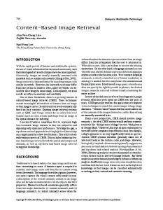
(a) Figure 2. Two images and their corresponding points
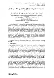
(b) Figure 1. Feature vector storing amplitudes (a) Cyclic permutation of the subvectors (b)
We changed this method by explicitely searching for corresponding points in both images. The means to qualify two points as being a pair is the minimum distance in feature space. To do this we build a matrix which stores the distances of all possible feature pairs, the lines i denoting the key points of the query image, the columns j the key points of the compared image, and the elements Ei;j the distance between point i of the query image and point j of the compared image. The search for correspondance is done in a greedy manner: We search the minimum element of the matrix. The column and line number denote the first pair of corresponding interest points. Both column and line are deleted from the matrix, since these two points are not available for other pairs. Then we again search the minimum element of the remaining matrix. This algorithm is continued until the matrix vanishes or the minimum distance does not exceed a given threshold (There are no more points having a corresponding partner). The distance between the two images is calculated using the number of corresponding points found:
method is based on texture feature vectors built from the output of the Gabor filter bank, each feature vector corresponding to one interest point. The 3 � 8 elements of a vector represent the responses of the 3 � 8 sized filter bank, where each element holds the maximum amplitude of a filter response. We compare two vectors in feature space. We split the vector into 3 parts, one for each scale. The subvectors contain 8 entries, one for each orientation (Figure 1). They can be interpreted as points in a 8 dimensional feature space. Thus, can be expressed by the Euclidean distance (�i �i )2 (� and � denote two subvecdE (�; � ) = i tors). We introduce a cyclic permutation to compensate for rotation. So the distance between two feature subvectors � and � is actually the minimum of 3 distances: 1
pP
dist(�; � ) = minfd (�; � ); d (per(�); � ); d (�; per(� ))g E
E
E
d(A; B ) =
where per(x) is a cyclic permutation of the vector x one element clockwise (Figure 1.b). The distance of the entire vectors, i.e. all 3 scales, is calculated as mean of the subvectors for each scale. Having found a suitable distance between two feature vectors, we need to define a distance between two images, which are described by two sets of feature vectors. Schmidt and Mohr used a voting algorithm: Each vector Vi of the query image is compared to all vectors Vj in the database, which are linked to their images Mk . If the distance between Vi and Vj is below a threshold t then the respective image Mk gets a vote. The images having maximum votes are returned to the user.
2
� Number of corresponding Points N (A) + N (B )
where N (A) denotes the number of interest points of the image A. The cost of the algorithm is O(N 2 ) for calculating the distance matrix plus the cost for the search of the corresponding pairs, which depends on the similarity of the two images. The higher the similarity the higher the cost, since the search for the minimum distance in the matrix has to be done more often. Still the overall cost of the search algorithm is O(N 2 log (N )).
3.2. Images as sets of histograms Motivated by the drawback of the computational expensive distance method presented in the last chapter we developed a histogram based representation and comparison
1 Classic
image indexation applications like video indexing, are not interested in a complete rotational invariance but must take into account small variations of orientations ( 22o in our implementation).
�
2
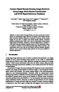
Figure 3. Image (a) and histograms for and 45o (c)
0o
(b)
technique, which uses the same output of the Gabor filter bank. In the feature vector set representation our data (i.e. the responses of the Gabor filter bank) was ordered by interest points. We now re-order the data by scales and orientations of the filter bank, and get for each combination of scale and orientation a distribution of maximum amplitudes — the responses for all interest regions to the filter for this scale and orientation. This information, which represents one image, can be stored in a set of 24 histograms ordered by filter index. The responses of one filter are embedded in a single two dimensional histogram. To fill one histogram all interest points are taken. For each point the n-nearest neighbour search (using spatial distance) is performed. The result of this search are n pairs of interest points, whose amplitudes we insert into the histogram. The maximum amplitude of the first point is used to calculate the bin index of the first dimension, and the maximum amplitude of the respective neighbour for the bin index of the second dimension. Figure 3 shows an example image and two 2D histograms out of its 24 histograms. The images’ fourier analysis contains frequencies mainly in the horizontal orientation (orientation 0). Therefore the histogram for orientation 0 shows strong responses, i.e. high bins from indices 4 to 6. The histogram for orientation index 2, which corresponds to structures in orientations around 45 degrees, shows only one high bin at index (0; 0), i.e. almost no response. The comparison of two images is based on already known distance measurements of histograms and their means. For the single histogram distances we used the Battacharrya distance, which performed slightly better than the L2 distance, thus confirmed results of Huet and Hancock [5]. We included some compensation for rotation by comparing each histogram not only with its corresponding histogram but as well with the immediate neighbours of the same scale, similar to the feature vector approach (Figure 1.b). We can represent our ordered set of 3 � 8 histograms as a set of 3 vectors, each containing 8 histograms. By cyclic permutation of each of these vectors and taking the minimum of comparison and comparison with one rotated vector, we get the final distance.
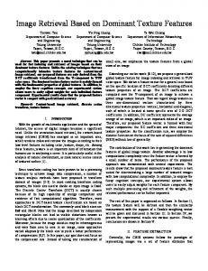
Figure 4. Examples of the image database
4. Experimental Results Our test database contains 609 images grabbed from a French television channel. The images are all of the same format (384x288 pixels) and coded in JPEG with 75% quality. The contents differs from outdoor activities (reports of sports) to talk shows, full scope shots of people, weather forecasts, logos and advertisements. To be able to measure a query performance a clustering of the image set was necessary. The clusters contain images of successive sequences. In fact, the pictures of one cluster mostly are taken from the same program and sometimes even from the same scene. Figure 4 shows examples of these groups. One column of the matrix contains images of the same cluster. Although all images of the database are compared during a query not all of them are grouped into clusters and used as query images. The reason is to avoid too small groups, which would degrade the query performance curves without justification. Eliminating all clusters with less than 10 images, the remaining 568 images are grouped into 11 clusters with the following sizes: 1 10
2 11
3 14
4 15
5 15
6 19
7 32
8 36
9 86
10 156
11 174
Since there is no general definition for visual similarity between images, measuring retrieval performance is a difficult task and depends on the purpose. A single query uses one image out of a cluster C , which contains d images. The system answers with images of which r are from the original cluster C . We use a measure which is widely used for indexation systems: precision.
P 3
=
r
As the name suggests, the precision of the result of a single query denotes how precise the result set responds to the desires of the user. By changing the size of the result set we get a performance curve for this query. We calculate the final curve for a retrieval method by averaging the curves for all single queries using different query images. Figure 5 displays curves for both retrieval methods The first method (5.b) performs slightly better than the histogram based method (5.c). However, it takes 37 seconds to compare one query image against the database of 609 images (standard PC, 300 MHz), whereas the second method finishes within 5.1 seconds. The curves are displayed together with the theoretical limits of query performance. A logical lower bound is the performance of a method selecting random images. (5.d). The upper boundary shows the performance of a query that picks all similar images if possible. This curve depends on the clustering of the database. A constant performance of 100% is only possible, if all clusters contain at least as many images as we retrieve in our result sets.
100
Upper limit
Average Precision (%)
80
Feature vectors 60
Histogram sets 40
Random images
20
Number of images in the return set 0 0
5
10
15
20
25
30
35
40
45
Figure 5. Precision using different methods
[5] B. Huet and E. Hancock. Cartographic indexing into a database of remotely sensed images. In Third IEEE Workshop on Applications of Computer Vision (WACV96), pages 8–14, Sarasota, Dec 1996. [6] J. Jolion and A. Montanvert. The adaptive pyramid, a framework for 2d image analysis. In Computer Vision, Graphics and Image Processing: Image Understanding, pages 55(3):339–348, May 1992. [7] W. Kropatsch. Building irregular pyramids by dualgraph contraction. IEE Proc.-Vis Image Signal Process., 142(6):366–374, December 1995. [8] E. Loupias, N. S. S. Bres, and J. Jolion. Wavelet-based salient points for image retrieval. In International Conference on Image Processing, Vancouver, Canada, 2000. [9] B. Manjunath and W. Ma. Texture features for browsing and retrieval of image data. IEEE Transactions on Pattern Analysis and Machine Intelligence, 18(8), August 1996. [10] H. Moravec. Towards automatic visual obstacle avoidance. In Proc. of 5th International Joint Conference on Artifical Intelligence, 584, page p. 587, 1977. [11] O. Popescu. Utilisation des points d’int´erˆet pour l’indexation d’images. Technical Report RR 99.07, Laboratoire Reconnaissance de Formes et Vision., 1999. [12] C. Schmidt and R. Mohr. Local gray value invariants for image retrieval. IEEE Transactions on Pattern Analysis and Machine Intelligence, 19(5), May 1997. [13] S. Siggelkow and H. Burkhard. Local invariant feature histograms. Technical Report IIF-LMB 01/98, AlbertLudwigs-Univ. Freiburg, Institut f. Informatik, Jan 1998. [14] S. Smith and J. Brady. Susan - a new approach to low level image processing. Int. Journal of Computer Vision, 23(1):45–78, May 1997. [15] M. Stricker and A. Dimai. Color indexing with weak spatial constraints. SPIE, 2670/29(0-8194-2044-1), 1996. [16] M. Swain and D. Ballard. Color indexing. International Journal of Computer Vision, 7(1):11–32, 1991. [17] C. Wolf. Content based image retrieval using interest points and texture features. Technical Report RR 99.09 (Forthcoming), Laboratoire Reconnaissance de Formes et Vision, 1999.
5. Conclusion and Outlook In this paper we presented two methods to use interest point detectors and a Gabor filter bank to create texture descriptions for image indexing. Both methods give good results according to our test image database. For indexation purposes the histogram based statistical method needs much less computational efforts, whereas the performance decrease is statistically not significant. Future work will integrate a structural component by combining the feature vector approach with attributed graph pyramids [6] [7]. Another task currently pursued is to join this texture based approach with methods based on colour, structure and shape into one weighted indexation system, which uses feedback of the user to determine the preferences and to recalculate the weights of the system [4].
References [1] S. Bhattacharjee. Image retrieval based on structural content. Technical Report SSC/1999/004, Dept. of Electrical Eng., E.P.F.L, CH-1015, Lausanne, 1999. [2] S. Bres and J. Jolion. Detection of interest points for image indexing. In 3rd Int. Conf. on Visual Inf. Systems, Visual 99, pages 427–434. Springer, Lecture Notes in Computer Science, 1614, June 1999. [3] C. Harris and M. Stephens. A combined corner and edge detector. In Proceedings 4th Alvey Visual Conference. Plessey Research Roke Manor, UK, 1988. [4] A. Heinrichs, D. Koubaroulis, B. Levienaise-Obadia, P. Rovida, and J. Jolion. Robust image retrieval in a statistical framework. Technical Report RR-99-04, Laboratoire Reconnaissance de Formes et Vision, Lyon, May 1999.
4
50