Context Aware Nonnegative Matrix Factorization Clustering (PDF ...

arXiv:1609.04628v1 [cs.CV] 15 Sep 2016

Context Aware Nonnegative Matrix Factorization Clustering Rocco Tripodi*

Sebastiano Vascon*

Marcello Pelillo

ECLT, Ca’ Foscari University Ca’ Minich 2940, Venice, Italy Email: [email protected]

ECLT, Ca’ Foscari University Ca’ Minich 2940, Venice, Italy Email: [email protected]

ECLT, Ca’ Minich 2940, Venice, Italy DAIS, Ca’ Foscari University Via Torino, Venice, Italy Email: [email protected]

Abstract—In this article we propose a method to refine the clustering results obtained with the nonnegative matrix factorization (NMF) technique, imposing consistency constraints on the final labeling of the data. The research community focused its effort on the initialization and on the optimization part of this method, without paying attention to the final cluster assignments. We propose a game theoretic framework in which each object to be clustered is represented as a player, which has to choose its cluster membership. The information obtained with NMF is used to initialize the strategy space of the players and a weighted graph is used to model the interactions among the players. These interactions allow the players to choose a cluster which is coherent with the clusters chosen by similar players, a property which is not guaranteed by NMF, since it produces a soft clustering of the data. The results on common benchmarks show that our model is able to improve the performances of many NMF formulations.

I. I NTRODUCTION Nonnegative matrix factorization (NMF) is a particular kind of matrix decomposition in which an input matrix X is factorized into two nonnegative matrices W and H of rank k, such that W H T approximates X. The significance of this technique is to find those vectors that are linearly independent in a determined vector space. In this way, they can be considered as the essential representation of the problem described by the vector space and can be considered as the latent structure of the data in a reduced space. The advantage of this technique, compared to other dimension reduction techniques such as Single Value Decomposition (SVD), is that the values taken by each vector are positive. In fact, this representation gives an immediate and intuitive glance of the importance of the dimensions of each vector, a characteristic that makes NMF particularly suitable for soft and hard clustering [1]. The dimensions of W and H T are n × k and k × m, respectively, where n is the number of objects, m is the number of features, and k is the number of dimensions of the new vector space. NMF uses different methods to initialize these matrices [2], [3], [4] and then optimization techniques are employed to minimize the differences between X and W H T [5]. The initialization of the matrices W and H [4], is crucial and can lead to different matrix decompositions, since it is performed randomly in many algorithms [6]. To the contrary, * = equal contribution.

the step involving the final clustering assignment received less attention by the research community. In fact, once W and H are computed, soft clustering approaches interpret each value in W as the strength of association among objects and clusters and hard clustering approaches assign each object j to the cluster Ck , where: k = arg max(Wj1 , Wj2 , ..., Wjk ).

(1)

This step is also crucial since in hard clustering it could be the case that the assignments have to be made choosing among very similar (possibly equal) values and Equation 1 in this case can results inaccurate or even arbitrary. Furthermore this approach does not guarantee that the final clustering is consistent, with the drawback that very similar objects can result in different clusters. In fact, the clusters are assigned independently with this approach and two different runs of the algorithm can result in different partitioning of the data, due to the random initializations [6]. These limitations can be overcome exploiting the relational information of the data and performing a consistent labeling. For this reason in this paper we use a powerful tool derived from evolutionary game theory, which allows to re-organize the clustering obtained with NMF, making it consistent with the structure of the data. With our approach we impose that the cluster membership has to be re-negotiated for all the objects. To this end, we employ a dynamical system perspective, in which it is imposed that similar objects have to belong to similar clusters, so that the final clustering will be consistent with the structure of the data. This perspective has demonstrated its efficacy in different semantic categorization scenarios [7], [8], which involve a high number of interrelated categories and require the use of contextual and similarity information. II. NMF C LUSTERING NMF is employed as clustering algorithm in different applications. It has been successfully applied in parts-of-whole decomposition [2], object clustering [9], face recognition [10], multimedia analysis [11], and DNA gene expression grouping [12]. It is an appealing method because it can be used to perform together objects and feature clustering. The generation of the factorized matrices starts from the assumption that the objects of a given dataset belong to k clusters and that

these clusters can be represented by the features of the matrix W , which denotes the relevance that each cluster has for each object. This description is very useful in soft clustering applications because an object can contain information about different clusters in different measure. For example a text about a the launch of a new car model into the marked can contain information about economy, automotive or life-style, in different proportions. Hard clustering applications require to choose just one of these topics to partition the data and this can be done considering not only the information about the single text, but also the information of the other texts in the texts collection, in order to divide the data in coherent groups. In many algorithms the initialization of the matrices W and H is done randomly [2] and have the drawback to always lead to different clustering results. In fact, NMF converges to local minima and for this reason has to be run several times in order to select the solution that approximates better the initial matrix. To overcome this limitation there were proposed different approaches to find the best initializations based on feature clustering [3] and SVD techniques [4]. These initializations allow NMF to converge always to the same solution. [3] uses spherical k-means to partition the columns of X into k clusters and selects the centroid of each cluster to initialize the corresponding column of W . Nonnegative Double Singular Value Decomposition (NNDSVD) [4] computes the k singular triplets of X, forms the unit rank matrices using the singular vector pairs, extracts from them their positive section and singular triplets and with this information initializes W and H. This approach has been shown to be almost as good as that obtained with random initialization [4]. A different formulation of NMF as clustering algorithm was proposed by [13] (SymNMF). The main difference with classical NMF approaches is that SymNMF takes a square nonnegative similarity matrix as input instead of a n × m data matrix. It starts from the assumption that NMF was conceived as a dimension reduction technique and that this task is different from clustering. In fact, dimension reduction aims at finding a few basis vectors that approximate the data matrix and clustering aims at partitioning the data points where similarity is high among the elements of a cluster and low among the elements of different clusters. In this formulation a basis vector strictly represents a cluster. Common approaches obtain an approximation of X minimizing the Frobenius norm of the difference ||X − W H T || or the generalized Kullback-Leibler divergence DKL (X||W H T ) [14] , using multiplicative update rules [15] or gradient methods [5]. III. G AME T HEORY AND G AME DYNAMICS Game theory was introduced by Von Neumann and Morgenstern [16] in order to develop a mathematical framework able to model the essentials of decision making in interactive situations. In its normal-form representation, it consists of a finite set of players I = {1, .., n}, a set of pure strategies for each player Si = {s1 , ..., sn }, and a utility function u : S1 × ... × Sn → R, which associates strategies to

payoffs. Each player can adopt a strategy in order to play a game and the utility function depends on the combination of strategies played at the same time by the players involved in the game, not just on the strategy chosen by a single player. An important assumption in game theory is that the players are rational and try to maximize the value of u. Furthermore, in non-cooperative games the players choose their strategies independently, considering what other players can play and try to find the best strategy profile to employ in a game. Nash equilibria represent the key concept of game theory and can be defined as those strategy profiles in which each strategy is a best response to the strategy of the co-player and no player has the incentive to unilaterally deviate from his decision, because there is no way to do better. The players can also play mixed strategies, which are probability distributions over pure strategies. A mixed strategy profile can be defined as a vector x = (x1 , . . . , xm ), where m is the number of pure strategies and each component xh denotes the probability that the player chooses its hth pure strategy. Each mixed strategy corresponds to a point on the simplex and its corners correspond to pure strategies. In a two-player game, a strategy profile can be defined as a pair (p, q) where p ∈ ∆i and q ∈ ∆j . The expected payoff for this strategy profile is computed as: ui (p, q) = p · Ai q , uj (p, q) = q · Aj p

(2)

where Ai and Aj are the payoff matrices of player i and j respectively. In evolutionary game theory we have a population of agents which play games repeatedly with their neighbors and update their beliefs on the state of the system choosing their strategy according to what has been effective and what has not in previous games, until the system converges. The strategy space of each player i is defined as a mixed strategy profile xi , as defined above. The payoff corresponding to a single strategy can be computed as: ui (ehi ) =

n X (Aij xj )h

(3)

j=1

and the average payoff is: ui (x) =

n X

xTi Aij xj

(4)

j=1

where n is the number of players with whom the games are played and Aij is the payoff matrix among player i and j. The replicator dynamic equation [17] is used in order to find those states, which correspond to the Nash equilibria of the games, u(eh , x) ∀h ∈ S (5) xh (t + 1) = xh (t) u(x, x) This equation allows better than average strategies to grow at each iteration and we can consider each iteration of the dynamics as an inductive learning process, in which the players learn from the others how to play their best strategy in a determined context.

NMF Clustering

GT NMF Clustering GT NMF

NMF

Dataset

Payoff matrix ×

≈ X

Strategy Space

H

W

S A

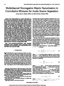
Fig. 1. The pipeline of the proposed game-theoretic refiner method: a dataset is clustered using NMF obtaining a partition of the original data into k clusters. A pairwise similarity matrix A is constructed on the original set of data and the clustering assignments obtained with NMF. The output of NMF (W ) and the matrix A are used to refine the assignments. The matrix W is also used to initialize the strategy space of the games. In red the wrong assignment that is corrected after the refinement. Best viewed in color.

IV. O UR A PPROACH In this section we present the Game Theoretic Nonnegative Matrix Factorization (GTNMF), our approach to NMF clustering refinement. The pipeline of this method is depicted in Fig. 1. We extract the feature vectors of each object in a dataset then, depending on the NMF algorithm used, we give as input to NMF the feature vectors or a similarity matrix. GTNMF takes as input the matrix W obtained with NMF and the similarity graph A (see Section V-C) of the dataset to produce a consistent clustering of the data. Each data point, in our formulation, is represented as a player that has to choose its cluster membership. The weighted graph A measures the influence that each player has on the others. The matrix W is used to initialize the strategy space S of w the players. We use the following equation sij = PK ijw ij j=1 to constrain the strategy space of each player to lie on the standard simplex, as required in a game theoretic framework (see Section III). The dynamics are not started on the center of the K-dimensional simplex, as it is commonly done in unsupervised learning tasks, but on a different interior point, which corresponds to the solution point of NMF and do not compromise the dynamics to converge to Nash equilibria [18]. Now that we have the topology of the data A and the strategy space of the game S we can compute the Nash equilibria of the games according to equation (5). In each iteration of the system each player plays a game with its neighbors Ni according to the similarity graph A and the payoffs are calculated as follows: X ui (eh , s) = (aij sj )h (6)

strategies with higher payoff to emerge and at the end of the process each player chooses its cluster according to these constraints. Since Equation 5 models a dynamical system it requires some criteria to stop. In the experimental part of this work we used as stopping criteria the maximum number of iterations = 100 and δ < 104 , where δ is the Euclidean norm between the strategy space at time t and at time t + 1. V. E XPERIMENTAL S ETUP AND R ESULTS In this section, we show the performances of GTNMF on different text and image datasets, and compare it with standard NMF1 [19], NMF-S [19] (same as NMF but with the similarity matrix as input instead of the features), SymNMF [13]2 and NNDSVD3 [4], which use the standard maximization technique to obtain an hard clustering of the data. In Table II we refer to our approach as NMF-algorithm+GT which means that the GTNMF has been initializied with the particular NMFalgorithm. A. Datasets description The evaluation of GTNMF has been conducted on datasets with different characteristics (see Table I). We used textual (Reuters, RCV1, NIPS) and image (COIL-20, ORL, Extended YaleB and PIE-Expr) datasets. Authors in [13] discarded the objects belonging to small clusters in order to make the dataset more balanced, simplifying the task. We tested our method using this approach and also keeping the datasets as they are (without reduction), which lead to situations in which it is possible to have in the same dataset clusters with thousands of objects and clusters with just one object (e.g. RCV1).

j∈Ni

B. Data preparation

and ui (s) =

X

xTi (aij sj )

(7)

j∈Ni

We assume that the payoff of player i depends on the similarity that it has with player j, aij , and its preferences, (sj ). During each phase of the dynamics a process of selection allows

The datasets have been processed as suggested in [13]. Given an n×m data matrix X, the similarity matrix A is constructed 1 Code:

https://github.com/kimjingu/nonnegfac-matlab https://github.com/andybaoxv/symnmf 3 Code: http://www.boutsidis.org/NNDSVD matlab implementation.rar 2 Code:

TABLE I DATASETS DESCRIPTION . F = THE DATASET HAS BEEN PRUNED AS IN [13]. Dataset NIPSF NIPS ReutersF Reuters RCV1F RCV1 PIE-Expr ORL COIL-20 ExtYaleB

Type text text text text text text image image image image

Points 424 451 8095 8654 13254 13732 232 400 1440 2447

Features 17522 17522 14143 14333 20478 20478 4096 5796 4096 3584

Clusters 9 13 20 65 40 75 68 40 20 38

according to the type of dataset (textual and image). With textual dataset each feature vector is normalized to have unit 2-norm and the cosine distance is computed, A = xi T xj . For image datasets each feature (column) is first normalized to lie in the range [0, 1] and then it is applied the following kernel: ||x −x || Ai,j = exp{− σi i σjj }, where σi is the Euclidean distance of the 7-th nearest neighbor [20]. In all cases Aii = 0. The matrix is thus sparsified keeping only the q nearest neighbors for each point. The parameter q is set accordingly to [21] and represents a theoretical bound that guarantees the connectedness of a graph: q = blog2 (n)c + 1

(8)

Let N (i) = {j s.t. xj ∈ q-NN of i} then Aij = Aij if i ∈ N (j) or j ∈ N (i) and 0 otherwise. The matrix A is thus normalized in√a normalized-cut fashion p Pn obtaining the final matrix Aij = Aij di dj where di = s=1 Ais . The matrix A is given as input to all the compared methods, expect from NMF to which the data matrix X is given. See [13] for further details on this phase. C. Games graph In Sec.V-B has been explained how to create the similarity matrix for NMF, the same methodology has been used to create the payoff matrix A for the GTNMF, with the only difference that, in this case, we exploit the partitioning obtained with NMF in order to identify what could be the expected size of the clusters. The assumption here is that the clustering obtained via NMF provides a good insight on the size of the final clusters and accordingly with this information a proper number q (see Equation 8) can be selected. A cluster C can be considered as a fully connected subgraph and thus the number of neighbors of each element in the cluster C should be at least qC = blog2 (|C|)c + 1 to guarantee the connectedness of the cluster itself. The variable q is thus chosen based on the same principle of [21] but instead of taking into account the entire set of points (as in Sec.V-B) we focused only on the subsets induced by the NMF clustering. This results in having a different q for each point in the dataset based on the following rule: qi = blog2 (|C|)c + 1 (9) where |C| is the cardinality of cluster C to which the i-th element belongs to. For obvious reason qi ≤ q , ∀i = 1, . . . , n

Balance 0.105 0.028 0.011 0 0.028 0.001 0.75 1 1 0.678

Mean Clust 47.1 34.7 404.8 133.1 331.4 183.1 3.4 10 72 64.4

Min Cl Size 15 4 42 1 45 1 3 10 72 59

Max Cl Size 143 143 3735 3735 1587 1587 4 10 72 87

and thus concentrating only on the potential number of neighbors that belong to the cluster and not in the entire graph because we are doing a refinement. From a game-theoretic perspective this means to focus the games only among a set of similar players which are likely to belong to the same cluster. D. Evaluation measures Our approach has been validated using two different measures, accuracy (AC) and normalized mutual information (NMI). Pn i=1 δ(αi ,map(li )) , where n denotes the AC is calculated as n total number of documents in the dataset, δ(x, y) equals to 1 if x and y are clustered in the same class; map(Li ) maps each cluster label li to the equivalent label in the benchmark. The best mapping is computed using the KuhnMunkres algorithm [22]. The AC counts the number of correct clusters assignments. NMI indicates the level of agreement between the clustering C provided by the ground truth and the clustering C 0 produced by a clustering algorithm. The mutual information (MI) between the two clusterings is computed as, X

p(ci , c0j ) · log2

ci ∈C,c0j ∈C 0

p(ci , c0j ) p(ci ) · p(c0j )

(10)

where p(ci ) and p(c0i ) are the probabilities that a document of the corpus belongs to cluster ci and c0i , respectively, and p(ci , c0i ) is the probability that the selected document belongs to ci as well as c0i at the same time. The MI information is then normalized with the following equation, N M I(C, C 0 ) =

M I(C, C 0 ) max(H(C), H(C 0 ))

(11)

where H(C) and H(C 0 ) are the entropies of C and C 0 , respectively. E. Evaluation The results of our evaluation are shown in Table II, where we reported the mean and standard deviation of 20 independent runs. For NNDSVD the experiments are run only one time, since it converges always to the same solution. The performances of GTNMF in most of the cases are higher those of the different NMF algorithms. In particular, we can notice that despite the different settings (textual/image datasets) our algorithm is able improve the NMI performance in 33/36 cases

TABLE II P ERFORMANCE OF GTNMF COMPARED TO SEVERAL NMF APPROACHES . T HE MEAN AND STD DEVIATION OF 20 RUNS ARE REPORTED . Dataset NIPS F NIPS Reuters F Reuters RCV1 F RCV1 PIE-Expr ORL COIL-20 ExtYaleB

SymNMF 0.385 (±0.011) 0.387 (±0.007) 0.502 (±0.014) 0.517 (±0.007) 0.406 (±0.007) 0.411 (±0.006) 0.95 (±0.004) 0.888 (±0.006) 0.871 (±0.009) 0.308 (±0.005)

SymNMF+GT 0.405 (±0.016) 0.418 (±0.017) 0.51 (±0.016) 0.525 (±0.006) 0.422 (±0.007) 0.422 (±0.006) 0.968 (±0.004) 0.921 (±0.006) 0.875 (±0.012) 0.313 (±0.005)

Dataset NIPS F NIPS Reuters F Reuters RCV1 F RCV1 PIE-Expr ORL COIL-20 ExtYaleB

SymNMF 0.462 (±0.013) 0.379 (±0.01) 0.517 (±0.044) 0.324 (±0.029) 0.292 (±0.015) 0.243 (±0.008) 0.81 (±0.021) 0.776 (±0.017) 0.727 (±0.036) 0.235 (±0.008)

SymNMF+GT 0.483 (±0.016) 0.415 (±0.037) 0.528 (±0.043) 0.363 (±0.032) 0.289(±0.014) 0.247 (±0.008) 0.85 (±0.019) 0.811 (±0.018) 0.729 (±0.037) 0.228(±0.007)

Normalized Mutual Information NMF NMF+GT NMFS 0.375 (±0.022) 0.386 (±0.011) 0.388 (±0.006) 0.401 (±0.016) 0.406 (±0.016) 0.393 (±0.008) 0.451 (±0.026) 0.49 (±0.02) 0.505 (±0.014) 0.442 (±0.006) 0.497 (±0.003) 0.518 (±0.006) 0.51 (±0.007) 0.516 (±0.005) 0.404 (±0.009) 0.462 (±0.009) 0.483 (±0.007) 0.413 (±0.006) 0.939 (±0.008) 0.959 (±0.006) 0.89 (±0.005) 0.691 (±0.015) 0.844 (±0.014) 0.889 (±0.006) 0.619 (±0.017) 0.669 (±0.016) 0.877 (±0.013) 0.356 (±0.006) 0.355(±0.007) 0.309 (±0.007) Accuracy NMF NMF+GT NMFS 0.426 (±0.02) 0.425(±0.014) 0.465 (±0.011) 0.396 (±0.022) 0.39(±0.018) 0.384 (±0.014) 0.322 (±0.024) 0.401 (±0.026) 0.516 (±0.037) 0.222 (±0.011) 0.282 (±0.02) 0.339 (±0.023) 0.383 (±0.009) 0.387 (±0.01) 0.298 (±0.017) 0.279 (±0.01) 0.295 (±0.011) 0.242 (±0.01) 0.783 (±0.023) 0.809 (±0.024) 0.617 (±0.019) 0.465 (±0.019) 0.608 (±0.026) 0.77 (±0.013) 0.478 (±0.023) 0.507 (±0.025) 0.739 (±0.046) 0.194 (±0.007) 0.197 (±0.009) 0.237 (±0.012)

with a maximum gain of ' 15.3% (which is quite impressive) and a maximum loss of 0.2%. constant gain in the NMI

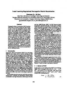
Fig. 2. On the left side a confusion matrix produced by NMF on the ORL dataset and on the right side the ones produced by our method.

means, in practice, that the algorithm is able to partition better the dataset, making the final clustering closer to the ground truth. In terms of AC, on 27/36 cases the method improve on the compared methods, with a maximum gain of 14.3% and maximum loss of 2.3%. It worth noting that the negative results are very low and in most of the cases the corresponding number of incorrect reallocations is low, in fact, −0.6% in the NIPS dataset means 2.7 elements or −0.2% in COIL-20 corresponds to 2.8 elements. The mean gain for NMI and AC are 2.68% and 2.30%, respectively, while the mean loss are 0.16% and 0.01%. In some cases we can see that we obtain a loss in NMI and a gain in AC, for example on ExtYaleB with NMF. In this case the similarity matrix given as input to GTNMF tends to concentrate more objects in the same cluster, because the dataset is not balanced and it could be the case that, in

NMFS+GT 0.403 (±0.007) 0.412 (±0.018) 0.511 (±0.015) 0.527 (±0.005) 0.42 (±0.01) 0.424 (±0.006) 0.931 (±0.006) 0.918 (±0.004) 0.883 (±0.013) 0.314 (±0.005)

NNDSVD 0.388 0.388 0.427 0.488 0.403 0.398 0.86 0.808 0.824 0.288

NNDSVD+GT 0.399 0.421 0.425 0.493 0.402 0.407 0.889 0.892 0.836 0.315

NMFS+GT 0.485 (±0.017) 0.407 (±0.031) 0.525 (±0.037) 0.378 (±0.024) 0.297(±0.017) 0.245 (±0.011) 0.7 (±0.02) 0.804 (±0.015) 0.741 (±0.046) 0.23(±0.01)

NNDSVD 0.474 0.466 0.403 0.277 0.285 0.239 0.536 0.653 0.674 0.229

NNDSVD+GT 0.509 0.503 0.427 0.339 0.276 0.24 0.513 0.71 0.672 0.242

these situations, a big cluster tends to attract many objects, increasing the probability of good reallocations, which results in an increase in AC and in a potentially wrong partitioning of the data. To the contrary in some experiments we have a loss in AC and a gain in NMI. For example on PIE-Expr we noticed that we are able to put together many objects that the other approaches tend to keep separated, but in this particular case GTNMF collected in the same cluster all the objects belonging to four similar clusters and for this reason there was a loss in accuracy (see Fig. 3). We can see that the results of our method on well balanced datasets (ORL, COIL-20) are almost always good. Also on very unbalanced datasets, such as Reuters and ReutersF we have always good performances, whatever is the method used. These datasets depict better real life situations and the improvements over them are due to the fact that in these cases it is necessary to exploit the geometry of the data in order to obtain a good partitioning. A positive and a negative case study are shown in Fig. 2 and 3, respectively. In Fig. 2 the confusion matrix obtained with GTNMF is less sparse and more concentrated on the main diagonal. Given the same cluster Id, the NMF method agglomerates different clusters (red arrows) while, after the refinement, the number of elements corresponding to the correct cluster are moved. In Fig. b the algorithm tends to agglomerates the elements on a single cluster (second column of the matrix). This can be explained on how the similarity matrix is composed and on the nature of the data: in Fig. c the std dev of the images in the agglomerated cluster is reported, as one can notice the std is very low meaning that all the faces in that cluster are very similar to each other. To give a counterexample we report on Fig. d the std dev of two random cluster joined together, is straightforward to notice that the std

Fig. 3. On a and b the confusion matrices produced by NMF and GTNMF on Pie-Expr. On c the std dev of the objects merged together by GTNMF and on d the std dev of two random clusters combined together.

dev is higher than in the previous example meaning that the elements within those two clusters are highly dissimilar in nature and thus easily separable. VI. C ONCLUSION In this work we presented GTNMF, a game theoretic model to improve the clustering results obtained with NMF going beyond the classical technique used to make the final clustering assignments. The W matrix obtained with NMF can have an high entropy which make the choice of a cluster very difficult in many cases. With our approach we try to reduce the uncertainty in the matrix W using evolutionary dynamics and taking into account contextual information to perform a consistent labeling of the data. In fact, with our method similar objects are assigned to similar clusters, taking into account the initial solution obtained with NMF. We conducted an extensive analysis of the performances of our method and compared it with different NMF formulations and on datasets with different features and of different kind. The results of the evaluation demonstrated that our approach is almost always able to improve the results of NMF and that when it have negative results those results are practically non significant. The algorithm is quite general thanks to the adaptive auto-tuning of the payoff matrix and can deal with balanced and completely unbalanced datasets. As future work we are planning to use different initialization of the strategy space, to use new similarity functions to construct the games graph, to apply this method to different problems and to different clustering algorithms. ACKNOWLEDGMENT This work was supported by Samsung Global Research Outreach Program. R EFERENCES [1] W. Xu, X. Liu, and Y. Gong, “Document clustering based on nonnegative matrix factorization,” in Proceedings of the 26th annual international ACM SIGIR conference on Research and development in informaion retrieval. ACM, 2003, pp. 267–273. [2] D. D. Lee and H. S. Seung, “Learning the parts of objects by nonnegative matrix factorization,” Nature, vol. 401, no. 6755, pp. 788–791, 1999. [3] S. Wild, J. Curry, and A. Dougherty, “Improving non-negative matrix factorizations through structured initialization,” Pattern Recognition, vol. 37, no. 11, pp. 2217–2232, 2004.

[4] C. Boutsidis and E. Gallopoulos, “Svd based initialization: A head start for nonnegative matrix factorization,” Pattern Recognition, vol. 41, no. 4, pp. 1350–1362, 2008. [5] C.-J. Lin, “Projected gradient methods for nonnegative matrix factorization,” Neural computation, vol. 19, no. 10, pp. 2756–2779, 2007. [6] Z.-Y. Zhang, T. Li, C. Ding, and J. Tang, “An nmf-framework for unifying posterior probabilistic clustering and probabilistic latent semantic indexing,” Communications in Statistics-Theory and Methods, vol. 43, no. 19, pp. 4011–4024, 2014. [7] R. Tripodi and M. Pelillo, “A game-theoretic approach to word sense disambiguation,” Computational Linguistics, in press. [8] R. Tripodi and M. Pelillo, “Document Clustering Games in Static and Dynamic Scenarios,” ArXiv e-prints, Jul. 2016. [9] C. Ding, T. Li, and W. Peng, “Nonnegative matrix factorization and probabilistic latent semantic indexing: Equivalence chi-square statistic, and a hybrid method,” in Proceedings of the national conference on artificial intelligence, vol. 21, no. 1. Menlo Park, CA; Cambridge, MA; London; AAAI Press; MIT Press; 1999, 2006, p. 342. [10] Y. Wang, Y. Jia, C. Hu, and M. Turk, “Non-negative matrix factorization framework for face recognition,” International Journal of Pattern Recognition and Artificial Intelligence, vol. 19, no. 04, pp. 495–511, 2005. [11] J. C. Caicedo, J. BenAbdallah, F. A. Gonz´alez, and O. Nasraoui, “Multimodal representation, indexing, automated annotation and retrieval of image collections via non-negative matrix factorization,” Neurocomputing, vol. 76, no. 1, pp. 50–60, 2012. [12] Z.-Y. Zhang, T. Li, C. Ding, X.-W. Ren, and X.-S. Zhang, “Binary matrix factorization for analyzing gene expression data,” Data Mining and Knowledge Discovery, vol. 20, no. 1, pp. 28–52, 2010. [13] D. Kuang, S. Yun, and H. Park, “Symnmf: nonnegative low-rank approximation of a similarity matrix for graph clustering,” Journal of Global Optimization, vol. 62, no. 3, pp. 545–574, 2015. [14] A. Berman and R. J. Plemmons, “Nonnegative matrices,” The Mathematical Sciences, Classics in Applied Mathematics, vol. 9, 1979. [15] D. D. Lee and H. S. Seung, “Algorithms for non-negative matrix factorization,” in Advances in neural information processing systems, 2001, pp. 556–562. [16] J. Von Neumann and O. Morgenstern, Theory of Games and Economic Behavior (60th Anniversary Commemorative Edition). Princeton University Press, 1944. [17] P. D. Taylor and L. B. Jonker, “Evolutionary stable strategies and game dynamics,” Mathematical biosciences, vol. 40, no. 1, pp. 145–156, 1978. [18] J. W. Weibull, Evolutionary game theory. MIT press, 1997. [19] J. Kim, Y. He, and H. Park, “Algorithms for nonnegative matrix and tensor factorizations: a unified view based on block coordinate descent framework,” Journal of Global Optimization, vol. 58, no. 2, pp. 285– 319, 2014. [20] L. Zelnik-Manor and P. Perona, “Self-tuning spectral clustering,” in Advances in neural information processing systems, 2004, pp. 1601– 1608. [21] U. Von Luxburg, “A tutorial on spectral clustering,” Statistics and computing, vol. 17, no. 4, pp. 395–416, 2007. [22] L. Lovasz and M. Plummer, “Matching theory north-holland mathematics studies, 121,” Annals of Discrete Mathematics, vol. 29, 1986.