Context-dependent effects on spatial variation in deer-vehicle collisions ANTHONY P. CLEVENGER,1,! MIRJAM BARRUETO,1 KARI E. GUNSON,2 FIONA M. CARYL,3
AND
ADAM T. FORD4
1
Western Transportation Institute, Montana State University, P.O. Box 174250, Bozeman, Montana 59717 USA 2 Eco-Kare International, 644 Bethune Street, Peterborough, Ontario K9H 4A3 Canada 3 Australian Research Centre for Urban Ecology, University of Melbourne, Melbourne 3010 VIC Australia 4 University of British Columbia, Biological Sciences Building, Room 4200, 6270 University Boulevard, Vancouver, British Columbia V6T 1Z4 Canada
Citation: Clevenger, A. P., M. Barrueto, K. E. Gunson, F. M. Caryl, and A. T. Ford. 2015. Context-dependent effects on spatial variation in deer-vehicle collisions. Ecosphere 6(4):47. http://dx.doi.org/10.1890/ES14-00228.1
Abstract. Identifying factors that contribute to the risk of wildlife-vehicle collisions (WVCs) has been a key focus of wildlife managers, transportation safety planners and road ecologists for over three decades. Despite these efforts, few generalities have emerged which can help predict the occurrence of WVCs, heightening the uncertainty under which conservation, wildlife and transportation management decisions are made. Undermining this general understanding is the use of study area boundaries that are incongruent with major biophysical gradients, inconsistent data collection protocols among study areas and species-specific interactions with roads. We tested the extent to which factors predicting the occurrence of deer-vehicle collisions (DVCs) were general among five study areas distributed over a 11,400-km2 region in the Canadian Rocky Mountains. In spite of our system-wide focus on the same genus (i.e., Odocoileus hemionus and O. virginianus), study area delineation along major biophysical gradients, and use of consistent data collection protocols, we found that large-scale biophysical processes influence the effect of localized factors. At the local scale, factors predicting WVC occurrence varied greatly between individual study areas. Distance to water was an important predictor of WVCs in three of the five study areas, while other variables had modest importance in only two of the five study areas. Thus, lack of generality in factors predicting WVCs may have less to do with methodological or taxonomic differences among study areas than the large-scale, biophysical context within which the data were collected. These results highlight the critical need to develop a conceptual framework in road ecology that can unify the disparate results emerging from field studies on WVC occurrence. Key words: Canadian Rocky Mountains; deer-vehicle collisions; highway; mitigation; Odocoileus hemionus; Odocoileus virginianus; predictive model; road ecology; scale; traffic safety; wildlife. Received 10 July 2014; revised 22 October 2014; accepted 3 November 2014; final version received 9 February 2015; published 9 April 2015. Corresponding Editor: D. P. C. Peters. Copyright: ! 2015 Clevenger et al. This is an open-access article distributed under the terms of the Creative Commons Attribution License, which permits unrestricted use, distribution, and reproduction in any medium, provided the original author and source are credited. http://creativecommons.org/licenses/by/3.0/ ! E-mail:
[email protected]
INTRODUCTION
have pronounced impacts on the abiotic (e.g., chemical effluents, hydrology, land forms) and biological processes in nearby ecosystems (Forman et al. 2003). For example, there are an estimated 1.5 million collisions per year between vehicles and large mammals in the USA (Conover et al. 1995, L-P Tardiff and Associates 2003,
Roads, highways and railways are pervasive features of human-occupied landscapes, occurring in the cities, rural areas and remote areas of most nations (Davenport and Davenport 2006). This infrastructure and the vehicles on them can v www.esajournals.org
1
April 2015 v Volume 6(4) v Article 47
CLEVENGER ET AL.
Huijser et al. 2007a). Despite decades of research aimed at identifying which factors explain and predict the occurrence of wildlife-vehicle collisions (WVCs), few generalities have emerged among species or study areas (Gunson et al. 2011). For example, the amount of forest cover increased deer (Odocoileus spp.) collisions in Illinois and Iowa, but not in Minnesota (Finder et al. 1999, Hubbard et al. 2000, Nielsen et al. 2003). Population density was the most important factor explaining moose (Alces alces)-vehicle collisions in Norway, but not Newfoundland (Joyce and Mahoney 2001, Rolandsen et al. 2011). These idiosyncrasies highlight the urgent need for road ecologists to identify the contextdependent processes giving rise to WVCs in different study areas and for different species. A critical first step to creating a general framework that can predict WVC occurrence is to address the methodological and biophysical (i.e., landscape and road characteristics) contexts within which data are collected (Forman et al. 2003, Seiler 2003). For example, measurement error (Gunson et al. 2009), differences in data collection protocols by researchers (Huijser et al. 2007b) or large-scale (i.e., landscape or region) biophysical differences among study areas (National Research Council 2005) may all contribute to why a particular variable increases, decreases or has no effect on WVC occurrence. The effects of methodological differences are readily addressed through consistent data collection protocols among studies (Huijser et al. 2007a, Gunson et al. 2009); however, incorporating large-scale biophysical variables into studies on WVCs remains a significant knowledge gap in road ecology research. One reason why large-scale biophysical variables are challenging to address in WVC studies is that data collection efforts are often constrained by political boundaries—a by-product of agency cooperation among different political entities associated with transportation networks. Often times political boundaries split important biophysical boundaries, potentially masking large- and local-scale processes that can affect the probability of WVCs. Large-scale processes include land-use patterns (e.g., urban, rural, wilderness), watershed boundaries, human population growth, and wildlife population density (Forman 1995, Collinge 2009). Local-scale prov www.esajournals.org
cesses can include road visibility, traffic volume, vehicle speed, habitat types, and topography (Forman et al. 2003). Understanding how these processes interact with one another requires, among other things, study area boundaries congruent with biophysical processes (Reiners and Driese 2004). We tested the extent to which factors predicting WVC occurrence were general among five study areas distributed over a 11,400 km2 region in the Canadian Rocky Mountains. Our goal was to first control for methodology and then to quantify the extent to which localized factors predicted WVC among and within study areas. We focused our efforts on WVCs involving animals from genus Odocoileus spp. (deer) and ensured that our study area boundaries were congruent with major shifts in biophysical variables (e.g., climate, elevation). We then tested the hypothesis that factors predicting WVC occurrence will be consistent among study areas with similar biophysical characteristics. We contrasted this hypothesis with the null expectation that WVCs are idiosyncratic and exhibit high residual spatial auto-correlation in statistical models.
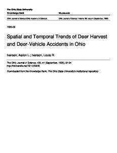
METHODS Study area The study area includes the mountainous landscapes of Banff, Kootenay and Yoho National Parks and adjacent Alberta provincial lands (Fig. 1; 50849 0 1100 to 51823 0 3800 N, 11589 0 4600 to 116829 0 700 W). The climate is continental and characterized by long winters and short summers (Holland and Coen 1983). We divided the landscape into five contiguous study areas, each with a major highway running along the valley bottom, and whose boundaries were derived from major watersheds (e.g., the continental divide) or abrupt transitions along biophysical gradients (i.e., elevation, valley width, valley orientation) (Table 1). The Trans-Canada Highway (TCH) is aligned west-east and transects two watersheds on either side of the Continental Divide, the Kicking Horse Valley and the Bow Valley (Banff National Park [BNP]). Highway 93 is aligned north-south in the Kootenay River drainage. Highway 40 is aligned north-south in the Kananaskis River Valley to the east of BNP. 2
April 2015 v Volume 6(4) v Article 47
CLEVENGER ET AL.
Fig. 1. Location of selected study areas and highways in the Canadian Rocky Mountains.
We divided the Bow Valley portion of the TCH into two regions based on biophysical transition: Bow-West in BNP and Bow-East outside BNP. Bow-West is characterized by higher elevation, greater precipitation, and lower human populav www.esajournals.org
tion density than Bow-East. At the time of data collection, there were both two- and four-lane highways and no wildlife exclosure fencing or wildlife crossing structures (Clevenger and Waltho 2005). 3
April 2015 v Volume 6(4) v Article 47
CLEVENGER ET AL. Table 1. Description of highways and traffic in five study areas of the Canadian Rocky Mountains. Highway
Study area
Trans-Canada Highway
Bow-East
Trans-Canada Highway
Bow-West
Trans-Canada Highway Highway 40
Kicking Horse Kananaskis
Highway 93 South
Kootenay
Political jurisdiction
Length (km)
Traffic volume (AADT)!
Posted speed (km hr"1)
35.1
16,960
110
32.2
8000
90
45.6 79.1
4600 3075"
90 90
102.6
2000
90
Province of Alberta, (east of Banff National Park) Banff National Park, Alberta (Highway 93 South junction to Yoho National Park boundary) Yoho National Park, British Columbia Province of Alberta (east of Banff National Park) Kootenay National Park, British Columbia
! AADT: 2005 annual average daily traffic volume (Parks Canada Agency and Alberta Transportation, unpublished data). " 1999 summer average daily traffic volume (Alberta Transportation, unpublished data).
and movement in an area nearby our study site. We also verified that white-tailed and mule deervehicle collisions co-occurred using the Williamson overlap index (Williamson 1993). The overlap index was 2.94, indicating that vehicle collisions with the two species were spatially correlated along each highway in study areas and thus could be grouped together.
Wildlife-vehicle collision data In January 1997, we collaborated with wildlife and highway managers in each study area to standardize WVC data collection. During regular operations, workers marked each WVC they encountered and reported the location to us. We subsequently visited the site and obtained a Universal Transverse Mercator coordinate using a differentially corrected global positioning system (GPS) unit (error , 3 m; Trimble Navigation, Sunnyvale, California, USA). We collected data on WVC locations for five ungulate species, and a total of 546 ungulate-vehicle collisions were reported between August 1997 and November 2003. However, we focused our analysis on deer, pooling data from mule deer (O. hemionus) and white-tailed deer (O. virginianus). Both deer species were prevalent in all study areas, comprised a large proportion (53%) of all WVCs, and we observed that these species have similar habitat requirements in our area. We expect that these two species may segregate among habitats, as do the sexes and age classes within species. However, our study addresses factors affecting WVCs, rather than habitat selection. There may be areas where these two species overlap, and other areas used exclusively, but the degree of segregation does not necessarily address the risk of WVC occurrence. WVC occurrence is shaped by an interaction of habitat selection, population abundance, and road variables (Forman et al. 2003, Seiler 2005, Gunson et al. 2011). Moreover, previous work in our study area by Lobo and Millar (2013) show that WVCs by these two deer species tend to occur in the same area, and Lingle (2002) showed that Odocoileus spp. overlap for foraging v www.esajournals.org
Predictor variables We identified 17 field and geographic information system (GIS)-derived variables that have been shown to affect the rate and location of DVCs in previous studies (Gunson et al. 2011) and measured these variables at 289 observed DVC locations and 721 random locations (Table 2). The number of random locations was proportionate (ca. 2:1) to the number of observed WVC locations of the original, multi-ungulate dataset in each study area. Measurement of field variables was obtained by first relocating each DVC and random location with a handheld GPS unit between April 2003 and February 2004 (Gunson et al. 2009). We used a rangefinder (Yardage Pro 1000, Bushnell, Denver, CO) to quantify visibility measurements variables in the field and an optical reading clinometer to measure slope.
Statistical analysis We measured collinearity of explanatory variables for each study area and calculated variance inflation factors (VIF; Zuur et al. 2010). We removed variables with a VIF ! 3.0 including: percentage of forest cover, shrub cover, and open area; in-line (5 m) visibility, angular visibility, and presence of barriers. Exploratory fitting of these 4
April 2015 v Volume 6(4) v Article 47
CLEVENGER ET AL. Table 2. Definition and description of variables selected to model occurrence of deer-vehicle collisions in five contiguous study areas of the Canadian Rocky Mountains. Predictor variable Continuous Forest! Shrub! Open! Cover! Human use" Barrier" Water" Road slope! Verge slope! Adjacent slope! In-line visibility! In-line visibility 5 m! Angular visibility! Road width! Categorical Habitat!
Topography! Barrier presence!
Definition Mean percentage (%) of continuous forest cover (trees .1 m height) in a 100-m transect perpendicular to highway, on both sides of highway. Mean percentage (%) of shrub cover (trees and shrubs ,1 m high) in a 100-m transect perpendicular to highway, on both sides of highway. Mean percentage (%) of area devoid of vegetation (rock, gravel, water, pavement etc.) in a 100-m transect perpendicular to highway, on both sides of highway. Mean distance (m) to vegetative cover (trees and shrubs .1 m high) on both sides of highway. Distance (m) to nearest human use feature along highway (parking areas, built areas, campgrounds, etc.). Distance (m) to nearest jersey or guardrail barrier. Distance (m) to nearest transverse waterway, i.e. drainage (river, stream, or creek). Mean slope (8) of land 0–5 m perpendicular to pavement edge, on both sides of highway. Mean slope (8) of land 5–10 m perpendicular to the pavement edge on both sides of highway. Mean slope (8) of land 10–30 m perpendicular to the pavement edge on both sides of highway. Mean distance observer at the pavement edge no longer sees passing vehicles, taken from each direction on both sides of highway. Mean distance at which observer at 5 m from pavement edge no longer sees passing vehicles, taken from each direction on both sides of highway. Mean distance at which observer at 10 m from the pavement edge no longer sees passing vehicles, taken from each direction on both sides of highway. Distance (m) between outer edges of road pavement. Dominant habitat within a 100-m radius on both sides of highway measured as forest (coniferous or deciduous forest); open-forest mix; open (fields, meadows, or barren ground); open-water area (wetland, lake, parallel stream or floodplain); riparian (perpendicular drainage), or rock. Adjacent terrain measured as level (1); completely raised and or buried (2, 3, 4), and partially raised or buried (5, 6). See Gunson et al. 2009 (Table 2). Number of concrete barriers and guard rails at site measured as 0, .1.
! Variable measured in field. " Variable measured from GIS.
for spatial coordinates), and (3) an interaction of study area and location. The study area term was used to quantify support for our initial characterization of the biophysical drivers of DVCs across this region; if our characterization was accurate and these large-scale processes mattered, then this factor should improve the null model. The location term addressed the extent to which DVCs were the result of spatially autocorrelated processes at the local scale (withinstudy area). We anticipated that deer abundance would vary at these local scales and to influence DVC occurrence. If factors predicting DVCs are driven by highly localized processes, then spatial coordinates should improve model fit. The model containing an interaction of the terms for studyarea and spatial coordinates addressed a synergy between the large-scale and local-scale processes giving rise to DVCs. Finally, to address the extent to which the factors predicting DVCs were general among study areas, we subdivided the large-scale data
data suggested that most predictor variables had non-linear relationships with the response variable. We therefore used Generalized Additive Models (GAM) to address these non-linear relationships, with cubic spline smoothing functions for all variables, and a logit link function with location type (i.e., observed or random) as the response variable. We were not only interested in which localscale factors predicted the location of WVCs, but the extent to which these factors were general within and between study areas. We first analysed DVCs at a large-scale by pooling data from the five study areas. We incorporated all non-collinear predictors, created models using all combinations of predictors and ranked model fit using Akaike’s Information Criterion (AICc) (Burnham and Anderson 2002). We defined the null model as the best-fitting model using these large-scale data. Next we considered how the fit of the null model is affected by: (1) study area, (2) location (i.e., a two-dimensional smoother term v www.esajournals.org
5
April 2015 v Volume 6(4) v Article 47
CLEVENGER ET AL. Table 3. A summary of models for each watershed analysis of deer-vehicle collisions with relative importance (RI) scores of nine explanatory variables. RI scores were calculated as the sum of model weights of all models containing a variable. Distance to: Study area
Water
Cover
Human use
Barrier
Slope angle
Visibility
Road width
Habitat
Topography
Bow East Bow West Kananaskis Kootenay Kicking Horse All areas Mean SD CV
0.58 0.92 0.28 0.22 0.96 0.98 0.65 0.34 0.53
0.44 0.26 0.27 0.64 0.4 0.11 0.35 0.18 0.51
0.48 0.31 0.27 0.42 0.24 0.14 0.31 0.12 0.39
0.99 0.41 0.46 0.68 0.48 0.99 0.66 0.26 0.39
0.08 0.9 0.31 0.54 0.84 0.19 0.47 0.34 0.71
0.68 0.34 0.29 0.68 0.24 0.22 0.41 0.21 0.52
0.94 0.52 0.35 0.44 0.29 0.65 0.53 0.23 0.44
0.02 0.08 0.61 * * 0.3 0.25 0.26 1.05
0.18 0.11 0.49 0.12 0.18 0.09 0.19 0.14 0.76
by study area and used model-selection procedures to identify the best-fitting model for each area. We calculated and compared a measure of relative importance of each variable (RI) as the sum of model weights across all possible models containing each variable, but we only reported models with DAICc , 2 (Anderson 2008).
Location (spatial coordinates) also improved the fit of the large-scale model (DAICc vs. null . 43), suggesting that DVCs are better predicted by factors operating at local scales. Ultimately, however, the best fitting model (DAICc vs. null . 48) was created from an interaction of study area and location, indicating that large-scale and local-scale processes operate synergistically to affect the location DVC locations.
RESULTS Collision summary data
Local-scale factors influencing DVC occurrence
Most of the 289 DVCs that we detected over the six-year study occurred in Bow-East (47%), followed by Kananaskis (18%), Bow-West (12%), Kootenay (12%), and Kicking Horse (10%). As a function of road-length and vehicle traffic (1000 annual average daily traffic volume [AADT]), the highest collision rate also occurred in Bow-East watershed (4.0 collisions km"1; 0.24 collisions km"1 1000 AADT"1), followed by Bow-West (1.1 collisions km"1 ; 0.14 collisions km"1 1000 AADT"1), Kananaskis (0.7 collisions km"1; 0.19 collisions km"1 1000 AADT"1), Kicking Horse (0.6 collisions km"1; 0.13 collisions km"1 1000 AADT"1), and Kootenay (0.3 collisions km"1; 0.15 collisions km"1 1000 AADT"1).
Factors predicting DVC occurrence varied greatly between individual study areas (Table 3). Distance to water was an important predictor of DVCs in three of the five study areas, while other variables (i.e., distance to barrier, slope, road width) had modest importance in only two of the five study areas. Topography, habitat, distance to cover and human use, and in-line visibility had little or no relative importance in any of the individual study area watershed models. When we included a smoothing term for spatial coordinates in the best-fitting model of each study area, there was meaningful improvement (DAICc ! 2) in three of the five study areas. This result indicates that, in addition to the 17 GIS- and field-derived variables we tested, there were one or more significant and unmeasured factors affecting DVC occurrence at a local scale (Table 3).
Large-scale factors influencing DVC occurrence The best-fitting model for the large-scale model included road width, distance to barrier, cover, topography, distance to water (drainage), and distance to human disturbance (Table 3; see Appendix: Table A1 for full results). The study area term improved the fit of this model (DAICc vs. null . 22), indicating that the biophysical boundaries we defined was associated with factors influencing DVCs (Appendix: Fig. A1). v www.esajournals.org
Residual spatial autocorrelation We tested for residual spatial autocorrelation (RSA) using spline correlograms (Bjornstad and Falck 2001) and Pearson’s residuals from the fitted best models (Bjornstad 2012). In the best6
April 2015 v Volume 6(4) v Article 47
CLEVENGER ET AL.
fitting model for the regional analysis, we found significant RSA for DVCs at a distance of ca. 17 m (Appendix: Fig. A2). We found no significant RSA in the best-fitting models for the individual study areas (with spatial coordinates included in the Bow-East and Kootenay models), suggesting that spatial dependencies between data points were accounted for appropriately in these models (Appendix: Figs. A2 and A3).
(i.e., large-scale) and road section (i.e., localscale) of interest. Road ecology theory predicts that WVCs arise from the occurrence of wildlife on the road, driver behavior and traffic volume (Forman et al. 2003). The occurrence of wildlife on the road is a function of variables such as wildlife population size, movement behavior and habitat type (Jaarsma et al. 2006, Found and Boyce 2011, Rolandsen et al. 2011, Cook and Blumstein 2013). The relationship between these variables is complex (Garshelis 2000, Frair et al. 2005, Johnson et al. 2006, Fryxell et al. 2008), which may weaken predictions of WVC occurrence using data derived from other study areas. For instance, using a 31-year long monitoring study on moose-vehicle collisions (MVC), Rolandsen et al. (2011) found moose density was the more important factor explaining variation in MVCs, both within and between 17 counties in Norway. In addition, the spatiotemporal variation in MVC was positively correlated to traffic volume and snow depth and negatively related to winter temperatures. Traffic volume can also be highly patchy along otherwise homogenous stretches of road because of variation in traffic flow and driver behavior (Drew 1968, Leutzbach 1988, Van Langevelde and Jaarsma 2004). Moreover, most WVC studies, ours included, do little to consider how these predictive factors vary over time. A legacy of high WVCs occurrence in an area may depress local population abundance, thereby lowering the probability of wildlife on the road, and generating ‘cold spots’ of WVC occurrence (Litvaitis and Tash 2008, Eberhardt et al. 2013). Given the complexity of factors contributing towards WVC occurrence, we urge researchers to uncover the mechanistic pathways by which wildlife behavior and abundance, traffic volume and driver behavior give rise to WVC occurrence (Bouchard et al. 2009). Some of the predictor variables we tested were present in the best-fitting models of more than one study area. Specifically, distance to water (drainage) was a key predictor of DVCs in the regional watershed model and three of five study areas. Typically, occurrence of DVCs was greatest .2 km from a drainage; however, the distance from drainage at which DVCs were lowest varied among these three study areas at 0 m at Bow West, 300 m at Kicking Horse and approximately
Model validation To validate the adequacy of our models, we used Q-Q plots modified for analysis of logistic regression (Landwehr et al. 1984, Zuur et al. 2009). We simulated 1000 data sets from the fitted models, and plotted the fitted residuals from the original model fit against the median simulated ordered residuals. Points outside of the 95% confidence intervals indicated possible outliers, while major deviations from the 1:1 line with points outside the confidence bands indicated departures from the model assumptions. The empirical probability plots for the best models in each watershed were all within the confidence intervals and showed reasonably straight lines (Appendix: Fig. A4), with the possible exception of the Kootenay and Kicking Horse models (Appendix: Figs. A5–A9), where low sample sizes (and thus wide confidence bands) made it difficult to determine if the apparent departure from a straight line was problematic.
DISCUSSION We found compelling evidence that factors predicting DVCs are context dependent, with a strong interaction between large- and local-scale biophysical processes. We expected to find greater agreement in the composition of models among the five study areas for the following reasons: (1) study areas were contiguous and shared many important ecosystem properties, such as climatic envelope, levels of human disturbance, and the composition of plant and animal communities; (2) our monitoring focused on species from the same genus, that occur in similar areas throughout our study area (3) field data were collected using consistent methods among study areas. The lack of generality among our models suggests that accurate predictions of DVC occurrence will require data from the area v www.esajournals.org
7
April 2015 v Volume 6(4) v Article 47
CLEVENGER ET AL.
1 km at Bow East (Appendix: Figs. A7–A9). In many landscapes, particularly mountainous ones, large animals often move along riparian areas through the landscape, likely to minimize the energetic costs of movement (Chruszcz et al. 2003, Dickson et al. 2005, Brost and Beier 2012). This suggests that drainages may increase DVC occurrence by concentrating wildlife movement across roads in highly localized areas. As such, mitigation measures aimed at increasing the safe passage of animals across the road in these areas may be more effective than influencing other predictors of DVC occurrence, such as driver behavior. In addition to factors that concentrate animal movements over particular stretches of highway, factors that increase the time required by wildlife to cross a highway appear to be particularly important in areas with high traffic volumes. For example, in Bow-East, which has 100% more traffic than then next busiest highway (BowWest), both barriers and road width increased probability of DVC occurrence. These variables were less important on highways with lower traffic volumes. These results are consistent with theoretical models that consider how animal body size, movement speed, traffic volume and road width influence DVC (Van Langevelde and Jaarsma 2004). Mitigation measures along roads characterized by high traffic volume should therefore focus on deterring wildlife access to the road surface, i.e., with exclusion fencing (Clevenger et al. 2001, Olsson and Widen 2008, McCollister and Van Manen 2010, Gagnon et al. 2011). Researchers in the emerging discipline of road ecology are being called upon to help design sustainable road systems and to mitigate the ecological effects of expanding transportation infrastructure (Sanderson et al. 2002, Ritters and Wickham 2003, Laurance et al. 2009). To reduce the occurrence of WVCs will therefore require knowledge of what processes contribute to their occurrence and ways to change the outcome of these processes. Our finding, that these processes interact at large and local-scales, suggests that there is a continued need for long-term monitoring of WVCs in areas where road and wildlifesafety are a priority. In the future, these monitoring studies will provide the empirical foundation required to develop a general understanding v www.esajournals.org
of factors causing WVCs.
ACKNOWLEDGMENTS Data collection for this study was part of a larger research project funded by Parks Canada and Public Works and Government Services Canada (contracts C8160-8-0010 and 5P421-010004/001). Funding from the partnership between Parks Canada (Banff National Park), the Henry P Kendall Foundation, Woodcock Foundation and Wilburforce Foundation enabled this research in the Canadian Rocky Mountains. We thank the Parks Canada warden service, Alberta Sustainable Resource Development conservation officers, VolkerStevin highway maintenance contractors for their help with reporting and marking the location of vehicle collisions with wildlife. We thank Cristina Mata, JeanYves Dionne and Ben Dorsey for assisting with collection of field-based measurements on highways in the study area. Jesse Whittington provided helpful comments on an earlier version of the paper. Bryan Chruszcz helped conceive and design the initial study. Jon Jorgenson, Alan Dibb, and Tom Hurd helped with additional data collection needs and logistics.
LITERATURE CITED Anderson, D. R. 2008. Model based inference in the life sciences. Springer, New York, New York, USA. Bjornstad, O. N. 2012. ncf: spatial nonparametric covariance functions. R package version 1.1-4. http://CRAN.R-project.org/package¼ncf Bjornstad, O. N., and W. Falck. 2001. Nonparametric spatial covariance functions: estimation and testing. Environmental and Ecological Statistics 8:53– 70. Bouchard, J., A. T. Ford, F. Eigenbrod, and L. Fahrig. 2009. Behavioral responses of Northern Leopard frogs (Rana pipiens) to roads and traffic: Implications for population persistence. Ecology and Society 14(2):1–10. Brost, B. M., and P. Beier. 2012. Use of land facets to design linkages for climate change. Ecological Applications 22:87–103. Burnham, K. P., and D. R. Anderson. 2002. Model selection and multimodal inference: a practical information-theoretic approach. Second edition. Springer Verlag, New York, New York, USA. Chruszcz, B., A. P. Clevenger, K. G. Gunson, and M. Gibeau. 2003. Relationships among grizzly bears, highways, and habitat in the Banff-Bow Valley, Alberta, Canada. Canadian Journal of Zoology 81:1378–1391. Clevenger, A. P., B. Chruszcz, and K. G. Gunson. 2001. Highway mitigation fencing reduces wildlife-vehicle collisions. Wildlife Society Bulletin 29:646–653.
8
April 2015 v Volume 6(4) v Article 47
CLEVENGER ET AL. Clevenger, A. P., and N. Waltho. 2005. Performance indices to identify attributes of highway crossing structures facilitating movement of large mammals. Biological Conservation 121:453–464. Collinge, S. K. 2009. Ecology of fragmented landscapes. Johns Hopkins University Press, Baltimore, Maryland, USA. Conover, M. R., W. C. Pitt, K. K. Kessler, T. J. DuBow, and W. A. Sanborn. 1995. Review of human injuries, illnesses and economic losses caused by wildlife in the U.S. Wildlife Society Bulletin 23:407– 414. Cook, T. C., and D. T. Blumstein. 2013. The omnivore’s dilemma: Diet explains variation in vulnerability to vehicle collision mortality. Biological Conservation 167:310–315. Davenport, J., and J. L. Davenport, editors. 2006. The ecology of transportation: managing mobility for the environment. Springer, London, UK. Dickson, B. G., J. S. Jenness, and P. Beier. 2005. Influence of vegetation, topography and roads on cougar movement in southern California. Journal of Wildlife Management 69:264–276. Drew, D. R. 1968. Traffic flow theory and control. McGraw-Hill, New York, New York, USA. Eberhardt, E., S. Mitchell, and L. Fahrig. 2013. Road kill hotspots do not effectively indicate mitigation locations when past road kill has depressed populations. Journal of Wildlife Management 77:1353–1359. Finder, R. A., J. L. Roseberry, and A. Woolf. 1999. Site and landscape conditions at white-tailed deervehicle collision locations in Illinois. Landscape and Urban Planning 44:77–85. Forman, R. T. T. 1995. Land mosaics: The ecology of landscapes and regions. Cambridge University Press, Cambridge, UK. Forman, R. T. T., et al. 2003. Road ecology: Science and solutions. Island Press, Washington, D.C., USA. Found, R., and M. S. Boyce. 2011. Predicting deervehicle collisions in an urban area. Journal of Environmental Management 92:2486–2493. Frair, J. L., E. H. Merrill, D. R. Visscher, D. Fortin, H. Beyer, and J. M. Morales. 2005. Scales of movement by elk (Cervus elaphus) in response to heterogeneity in forage resources and predation risk. Landscape Ecology 20:273–287. Fryxell, J. M., M. Hazell, L. Borger, B. Dalziel, D. Haydon, J. Morales, T. McIntosh, and R. Rosatte. 2008. Multiple movement modes by large herbivore at multiple spatial scales. Proceedings of the National Academy of Sciences 105:19114–19119. Gagnon, J. W., N. L. Dodd, and K. S. Ogren. 2011. Factors associated with use of wildlife underpasses and importance of long-term monitoring. Journal of Wildlife Management 75:1477–1487. Garshelis, D. L. 2000. Chapter 4. Delusions in habitat v www.esajournals.org
evaluation: measuring use, selection, and importance. Pages 111–164 in L. Boitani and T. K. Fuller, editors. Research techniques in animal ecology: Controversies and consequences. Columbia University Press, New York, New York, USA. Gunson, K., A. P. Clevenger, A. T. Ford, J. Bissonette, and A. Hardy. 2009. A comparison of data sets varying in spatial accuracy used to predict the occurrence of wildlife-vehicle collisions. Environmental Management 44:268–277. Gunson, K. E., G. Mountrakis, and L. Quackenbush. 2011. Spatial wildlife-vehicle collision models: A review of current work and its application to transportation mitigation projects. Journal of Environmental Management 92:1074–1082. Holland, W. D., and G. M. Coen. 1983. Ecological land classification of Banff and Jasper national parks. Volume III. The Wildlife Inventory. Canadian Wildlife Service, Edmonton, Alberta, Canada. Hubbard, M. W., B. J. Danielson, and R. A. Schmitz. 2000. Factors influencing the location of deervehicle accidents in Iowa. Journal of Wildlife Management 64:707–712. Huijser, M. P., P. McGowen, J. Fuller, A. Hardy, A. Kociolek, A. P. Clevenger, D. Smith, and R. Ament. 2007a. Wildlife-vehicle collision reduction study. Federal Highway Administration, Washington, D.C., USA. Huijser, M. P., J. Fuller, W. E. Wagner, A. Hardy, and A. P. Clevenger. 2007b. Animal-vehicle collision data collection: a synthesis of highway practice. National Cooperative Highway Research Program Synthesis 370. Transportation Research Board, Washington, D.C., USA. Jaarsma, C. F., F. van Langevelde, and J. Botma. 2006. Flattened fauna and mitigation: Traffic victims related to road, vehicle and species characteristics. Transportation Research Part D 11:264–276. Johnson, C. J., K. L. Parker, D. C. Heard, and M. P. Gillingham. 2006. Unrealistic animal movement rates as behavioural bouts: a reply. Journal of Animal Ecology 75:303–308. Joyce, T. L., and S. P. Mahoney. 2001. Spatial and temporal distributions of moose-vehicle collisions in Newfoundland. Wildlife Society Bulletin 29:281– 290. Landwehr, J. M., D. Pregibon, and A. C. Shoemaker. 1984. Graphical methods for assessing logistic regression models. Journal of American Statistical Association 79:61–71. Laurance, W. F., M. Goosem, and S. G. W. Laurance. 2009. Impacts of roads and linear clearings on tropical forests. Trends in Ecology and Evolution 24:659–669. Leutzbach, W. 1988. Introduction to the theory of traffic flow. Springer-Verlag, Berlin, Germany. Lingle, S. 2002. Coyote predation and habitat segrega-
9
April 2015 v Volume 6(4) v Article 47
CLEVENGER ET AL. tion of white-tailed and mule deer. Ecology 83:2037–2048. Litvaitis, J. A., and J. P. Tash. 2008. An approach toward understanding wildlife-vehicle collisions. Environmental Management 42:688–697. Lobo, N., and J. S. Millar. 2013. Summer roadside use by white-tailed deer and mule deer in the Rocky Mountains, Alberta. Northwestern Naturalist 94:137–146. L-P Tardiff and Associates. 2003. Collisions involving motor vehicles and large animals in Canada. Final report to Transport Canada Road Safety Directorate, Ottawa, Ontario, Canada. McCollister, M., and F. T. Van Manen. 2010. Effectiveness of wildlife underpasses and fencing to reduce wildlife-vehicle collisions. Journal of Wildlife Management 74:1722–1731. National Research Council. 2005. Assessing and managing the ecological impacts of paved roads. National Academies Press, Washington, D.C., USA. Nielsen, C. K., R. G. Anderson, and M. D. Grund. 2003. Landscape influences on deer-vehicle accident areas in an urban environment. Journal of Wildlife Management 67:46–51. Olsson, M. P. O., and P. Widen. 2008. Effects of highway fencing and wildlife crossings on moose Alces alces movements and space use in southwestern Sweden. Wildlife Biology 14:111–117. Reiners, W. A., and K. L. Driese. 2004. Flow and movements in nature: propagation of ecological influences through environmental space. Cambridge University Press, Cambridge, UK. Ritters, K. H., and J. D. Wickham. 2003. How far to the nearest road? Frontiers in Ecology and Environ-
v www.esajournals.org
ment 1:125–129. Rolandsen, C. M., E. J. Solberg, I. Herfindal, B. Van Moorter, and B.-E. Saether. 2011. Large-scale spatiotemporal variation in road mortality of moose: Is it all about population density? Ecosphere 2(10):113. Sanderson, E. W., M. Jaiteh, M. A. Levy, K. H. Redford, A. V. Wannebo, and G. Woolmer. 2002. The human footprint and the last of the wild. BioScience 52:891–904. Seiler, A. 2003. Effects of infrastructure on nature. Pages 31–50 in M. Trocme, editor. COST 341: Habitat fragmentation due to transportation infrastructure: The European Review. Office for Official Publication of the European Communities, Luxembourg. Seiler, A. 2005. Predicting locations of moose-vehicle collisions in Sweden. Journal of Applied Ecology 42:371–382. Van Langevelde, F., and C. F. Jaarsma. 2004. Using traffic flow theory to model traffic mortality in animals. Landscape Ecology 19:895–907. Williamson, C. E. 1993. Linking predation risk models with behavioural mechanisms: identifying population bottlenecks. Ecology 74:320–331. Zuur, A. F., E. N. Ieno, and C. S. Elphick. 2010. A protocol for data exploration to avoid common statistical problems. Methods in Ecology and Evolution 1:3–14. Zuur, A. F., E. N. Ieno, N. Walker, A. A. Saveliev, and G. M. Smith. 2009. Mixed effects models and extensions in ecology with R. Springer, New York, New York, USA.
10
April 2015 v Volume 6(4) v Article 47
CLEVENGER ET AL.
SUPPLEMENTAL MATERIAL APPENDIX A Table A1. A summary of all the possible generalized additive models for each study area analysis of deer-vehicle collisions with DAICc , 2. Model rank is the model rank order based on AICc; D2 is the proportion of deviance explained by each model; AICc is the corrected Akaike Information Criterion; DAICc is the difference between model AICc and the minimum AICc; w is the model AICc weight. Predictor variables are: (1) distance to water; (2) distance to cover;(3) distance to human use;(4) distance to barrier;(5) slope; (6) visibility; (7) road width; (8) habitat type; (9) topography; (10) study area, for regional analysis only.
Study area Bow East Bow West
Kananaskis
Kootenay
Kicking Horse
All areas
Model rank 1 1 2 3 4 5 6 7 8 9 1 2 3 4 5 6 7 8 9 10 11 12 13 1 2 3 4 5 6 7 8 9 10 11 1 2 3 4 5 6 7 8 9 10 1 2 3 4 5
Predictor variable 1 x x x x x x x x x x
2
3
4
5
x x x x x x x
x x x x x x x x x
6
7
x
x x
x
x x x
x
8
9
10
D2
AICc
DAICc
w
x x x x x
0.14 0.12 0.11 0.15 0.13 0.13 0.09 0.12 0.12 0.12 0.08 0.08 0.04 0.08 0.09 0.08 0.05 0.08 0.08 0.08 0.08 0.08 0.03 0.15 0.17 0.11 0.13 0.14 0.16 0.10 0.10 0.12 0.15 0.09 0.25 0.23 0.25 0.24 0.23 0.25 0.23 0.25 0.23 0.25 0.11 0.10 0.10 0.10 0.10
447.8 184.3 185.2 185.5 185.6 185.6 185.7 185.8 186.0 186.2 174.4 174.6 175.4 175.8 175.9 176.1 176.1 176.1 176.2 176.3 176.3 176.4 176.4 173.6 173.9 174.0 174.2 174.3 174.7 175.2 175.5 175.5 175.5 175.5 109.2 109.2 110.1 110.3 110.8 111.1 111.1 111.1 111.1 111.2 1127.0 1127.9 1128.3 1128.4 1128.9
0.0 0.0 0.9 1.3 1.3 1.3 1.5 1.5 1.8 1.9 0.0 0.2 1.0 1.3 1.4 1.6 1.7 1.7 1.8 1.9 1.9 1.9 1.9 0.0 0.3 0.5 0.7 0.8 1.1 1.6 1.9 1.9 1.9 2.0 0.0 0.0 0.9 1.1 1.6 1.9 1.9 1.9 1.9 2.0 0.0 0.9 1.2 1.4 1.9
0.35 0.09 0.05 0.05 0.04 0.04 0.04 0.04 0.04 0.03 0.03 0.03 0.02 0.02 0.01 0.01 0.01 0.01 0.01 0.01 0.01 0.01 0.01 0.05 0.04 0.04 0.04 0.03 0.03 0.02 0.02 0.02 0.02 0.02 0.08 0.08 0.05 0.05 0.04 0.03 0.03 0.03 0.03 0.03 0.18 0.11 0.10 0.09 0.07
x x x x x
x
x x
x x x
x
x x x
x x x x x
x x x x x
x x x x x x x x x x x x x x x x x x
x
x x
x x x x x x x x x x x x x x x x
x x x
x
v www.esajournals.org
x x x x x x
x x x x x
x x x x x x x
x x x x x x x x x x x x x
x x
x x x x x
x x x x x x
x x x x x
x x x x
x x
11
x x x x x
x
April 2015 v Volume 6(4) v Article 47
CLEVENGER ET AL.
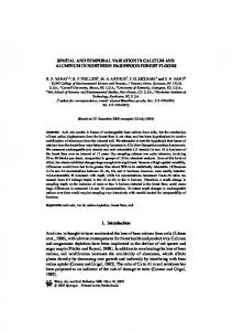
Fig. A1. Regional factors influencing WVC occurrence: Best fitting GAM for regional model, which included an interaction of biophysical study area and spatial coordinates. Dark red: probability of DVC ¼ 0, white-yellow: probability of DVC ¼ 1. GAM smoothing functions, with shaded areas delineating 95% confidence intervals. Term plots for parametric terms.
v www.esajournals.org
12
April 2015 v Volume 6(4) v Article 47
CLEVENGER ET AL.
Fig. A2. Spline correlograms for the residuals of the best-ranking GAM in each study area, with 95% confidence bands. Distance is in meters. Maximum considered distance was 2000 m in all models. The x-intercept, the distance beyond which objects are no more similar than what is expected by chance alone across the region, is given below the distance label. In brackets are the 95% confidence values.
v www.esajournals.org
13
April 2015 v Volume 6(4) v Article 47
CLEVENGER ET AL.
Fig. A3. Spline correlograms for the residuals of the best-ranking GAM in each study area, with 95% confidence bands. Spatial coordinates were included in the models for Bow-East, Kootenay and the All Study Area model. Distance is in meters. Maximum considered distance was 2000 m in all models. The x-intercept, the distance beyond which objects are no more similar than what is expected by chance alone across the region, is given below the distance label. In brackets are the 95% confidence values.
v www.esajournals.org
14
April 2015 v Volume 6(4) v Article 47
CLEVENGER ET AL.
Fig. A4. Quantile-quantile plots with 95% point-wise confidence bands for the best-ranking model of each analysis. The confidence bands were obtained by simulations of the fitted model. Number of simulations ¼ 1000. Black dots are residuals with value , 0.
v www.esajournals.org
15
April 2015 v Volume 6(4) v Article 47
CLEVENGER ET AL.
Fig. A5. Local-scale factors influencing WVC occurrence: Best fitting GAM for Kananaskis model, which included spatial coordinates. Dark red: probability of DVC ¼ 0, white-yellow: probability of DVC ¼ 1. GAM smoothing functions, with shaded areas delineating 95% confidence intervals. Term plots for parametric terms.
v www.esajournals.org
16
April 2015 v Volume 6(4) v Article 47
CLEVENGER ET AL.
Fig. A6. Local-scale factors influencing WVC occurrence: Best fitting GAM for Kootenay model, which included spatial coordinates. Dark red: probability of DVC ¼ 0, white-yellow: probability of DVC ¼ 1. GAM smoothing functions, with shaded areas delineating 95% confidence intervals.
v www.esajournals.org
17
April 2015 v Volume 6(4) v Article 47
CLEVENGER ET AL.
Fig. A7. Local-scale factors influencing WVC occurrence: Best fitting GAM for Kicking Horse model. GAM smoothing functions, with shaded areas delineating 95% confidence intervals.
v www.esajournals.org
18
April 2015 v Volume 6(4) v Article 47
CLEVENGER ET AL.
Fig. A8. Local-scale factors influencing WVC occurrence: Best fitting GAM for Bow-East model, which included spatial coordinates. Dark red: probability of DVC ¼ 0, white-yellow: probability of DVC ¼ 1. GAM smoothing functions, with shaded areas delineating 95% confidence intervals.
v www.esajournals.org
19
April 2015 v Volume 6(4) v Article 47
CLEVENGER ET AL.
Fig. A9. Local-scale factors influencing WVC occurrence: Best fitting GAM for Bow-West model. GAM smoothing functions, with shaded areas delineating 95% confidence intervals.
v www.esajournals.org
20
April 2015 v Volume 6(4) v Article 47