Context-Dependent Views to Axioms and Consequences of Semantic Web Ontologies Franz Baadera , Martin Knechtelb , Rafael Pe˜ nalozaa a Theoretical
Computer Science, TU Dresden, Germany b SAP AG, SAP Research
Abstract The framework developed in this paper can deal with scenarios where selected sub-ontologies of a large ontology are offered as views to users, based on contexts like the access rights of a user, the trust level required by the application, or the level of detail requested by the user. Instead of materializing a large number of different sub-ontologies, we propose to keep just one ontology, but equip each axiom with a label from an appropriate context lattice. The different contexts of this ontology are then also expressed by elements of this lattice. For large-scale ontologies, certain consequences (like the subsumption hierarchy) are often pre-computed. Instead of pre-computing these consequences for every context, our approach computes just one label (called a boundary) for each consequence such that a comparison of the user label with the consequence label determines whether the consequence follows from the sub-ontology determined by the context. We describe different black-box approaches for computing boundaries, and present first experimental results that compare the efficiency of these approaches on large real-world ontologies. Black-box means that, rather than requiring modifications of existing reasoning procedures, these approaches can use such procedures directly as sub-procedures, which allows us to employ existing highly-optimized reasoners. Similar to designing ontologies, the process of assigning axiom labels is error-prone. For this reason, we also address the problem of how to repair the labelling of an ontology in case the knowledge engineer notices that the computed boundary of a consequence does not coincide with her intuition regarding in which context the consequence should or should not be visible. Keywords: Access Restrictions, Views, Contexts, Ontologies
Description Logics (DL) [1] are a successful family of knowledge representation formalisms, which can be used to represent the conceptual knowledge of an application domain in a structured and formally well-understood way. They are employed in various application domains, such as natural language processing, conceptual modelling in databases, and configuration of technical systems, but their most notable success so far is the adoption of the DL-based language OWL as standard ontology language for the Semantic Web. From the DL point of view, an ontology is a finite set of axioms, which formalize our knowledge about the relevant concepts of the application domain. From this explicitly described knowledge, the reasoners implemented in DL systems can then derive implicit consequence. Application programs or human users interacting with the DL system thus have access not only to the explicitly represented knowledge, but also to its logical consequences. In order to provide fast access to the implicit knowledge, certain consequences (such as the subsumption hierarchy between named concepts) are often pre-computed by DLs systems.
In this paper, we investigate how this sort of precomputation can be done in an efficient way in a setting where users can access only parts of an ontology, and should see only what follows from these parts. To be more precise, assume that you have a large ontology O, but you want to offer different users different views on this ontology with respect to their context. In other words, each user can see only a subset of the large ontology, which is defined by the context she operates in. The context may be the level of expertise of the user, the access rights that she has been granted, or the level of detail that is deemed to be appropriate for the current setting, etc. More concretely, one could use context-dependent views for reducing information overload by providing only the information appropriate to the experience level of a user. For example, in a medical ontology we might want to offer one view for a patient that has only lay knowledge, one for a general practitioner, one for a cardiologist, one for a pulmonologist, etc. Another example is provided by proprietary commercial ontologies, where access is restricted according to a certain policy. The policy evaluates the context of each user by considering the assigned user roles, and then decides whether some axioms and the implicit consequences that can be derived from them are available to this user or not.
Email addresses:
[email protected] (Franz Baader),
[email protected] (Martin Knechtel),
[email protected] (Rafael Pe˜ naloza)
One na¨ıve approach towards dealing with such contextdependent views of ontologies would be to materialize a
1. Introduction
Preprint submitted to Special Issue of the Journal of Web Semantics on Reasoning with context in the Semantic Web
November 22, 2011
of pre-computing whether this consequence is valid for every possible sub-ontology, our approach computes just one label for each consequence such that a simple comparison of the context label with the consequence label determines whether the consequence follows from the corresponding sub-ontology or not. There are two main approaches for computing a boundary. The glass-box approach takes a specific reasoner (or reasoning technique) for an ontology language and modifies it such that it can compute a boundary. Examples for the application of the glass-box approach to specific instances of the problem of computing a boundary are tableau-based approaches for reasoning in possibilistic Description Logics [2, 3] (where the lattice is the interval [0, 1] with the usual order), glass-box approaches to axiom pinpointing in Description Logics [4, 5, 6, 7, 8] (where the lattice consists of (equivalence classes of) monotone Boolean formulae with implication as order [8]), and RDFS reasoning over labelled triples with modified inference rules for access control and provenance tracking [9, 10]. The problem with glass-box approaches is that they have to be developed and implemented for every ontology language and reasoning approach anew and optimizations of the original reasoning approach do not always apply to the modified reasoners. In contrast, the black-box approach can re-use existing optimized reasoners without modifications, and it can be applied to arbitrary ontology languages: one just needs to plug in a reasoner for this language. In this paper, we introduce three different black-box approaches for computing a boundary. The first approach uses an axiom pinpointing algorithm as black-box reasoner, whereas the second one modifies the Hitting-Set-Tree-based black-box approach to axiom pinpointing [11, 12]. The third uses binary search and can only be applied if the context lattice is a linear order. It can be seen as a generalization of the black-box approach to reasoning in possibilistic Description Logics described in [13]. Of course, the boundary computation only yields the correct results if the axiom labels have been assigned in a correct way. Unfortunately, just like creating ontology axioms, appropriately equipping these axioms with context labels is an error-prone task. For instance, in an access control application, several axioms that in isolation may seem innocuous could, together, be used to derive a consequence that a certain user is not supposed to see. If the knowledge engineer detects that a consequence c has an inappropriate boundary, and thus allows access to the consequence by users that should not see it, then she may want to modify the axiom labelling in such a way that the boundary of c is updated to the desired label. This problem is very closely related to the problem of repairing an ontology. Indeed, to correct the boundary of a consequence, one needs to be able to detect the axioms that are responsible for it, since only their labels have an influence on this boundary. In a large-scale ontology, this task needs to be automated, as analysing hundreds of thousands of
separate sub-ontology of the overall large ontology for each possible user context. However, this could potentially lead to an exponential number of ontologies having to be maintained, if we define one user context for each subset of the original ontology. This would imply that any update in the overall ontology needs to be propagated to each of the sub-ontologies, and any change in the context model, such as a new user role hierarchy or a new permission for a user role, may require removing or adding such subsets. Even worse, for each of these sub-ontologies, the relevant implicit consequences would need to be pre-computed and stored separately. To avoid these problems, we propose a different solution in this paper. The idea is to keep just the large ontology O, but assign “labels” to all axioms in the ontology and to all users in such a way that an appropriate comparison of the axiom label with the user label determines whether the axiom belongs to the sub-ontology for this user or not. This comparison will be computationally cheap and can be efficiently implemented with an index structure to look up all axioms with a given label. To be more precise, we use a set of labels L together with a partial order ≤ on L and assume that every axiom a ∈ O has an assigned label lab(a) ∈ L.1 The labels ℓ ∈ L are also used to define user contexts (which can be interpreted as access rights, required level of granularity, etc.). The sub-ontology accessible for the context with label ℓ ∈ L is defined to be O≥ℓ := {a ∈ O | lab(a) ≥ ℓ}. Clearly, the user of a DL-based ontology is not only able to access its axioms, but also the consequences of these axioms. That is, a user whose context has label ℓ should also be allowed to see all the consequences of O≥ℓ . As mentioned already, certain consequences are usually pre-computed by DL systems in order to avoid expensive reasoning during the deployment phase of the ontology. For example, in the version of the large medical ontology Snomed ct2 that is distributed to hospitals and doctors, all the subsumption relationships between the concept names occurring in the ontology are pre-computed. For a labelled ontology as introduced above, pre-computing that a certain consequence c follows from the whole ontology O is not sufficient. In fact, a user whose context has label ℓ should only be able to see the consequences of O≥ℓ , and since O≥ℓ may be smaller than O, the consequence c of O may not be a consequence of O≥ℓ . As said above, pre-computing consequences for all possible user labels is not a good idea since then one might have to compute and store consequences for exponentially many different subsets of O. Our solution to this problem is to compute a so-called boundary for the consequence c, i.e., an element ν of L such that c follows from O≥ℓ iff ℓ ≤ ν. Thus, instead 1 We will in fact impose the stronger restriction that (L, ≤) defines a lattice (see Section 2). 2 http://www.ihtsdo.org/snomed-ct/
2
axioms by hand is not feasible. To provide for such an automated label repair mechanism, we develop a black-box method for computing minimal sets of axioms that, when relabelled, yield the desired boundary for c; we call these minimal change sets. The main idea of this method is again based on the Hitting Set Tree (HST) algorithms that have been developed for axiom-pinpointing. However, we show that the original labelling function can be exploited to decrease the search space. This algorithm can be used to output all minimal change sets. The knowledge engineer can then choose which of them to use for the relabelling, depending on different criteria. Unfortunately, just as in axiompinpointing, there may be exponentially many such minimal change sets, and thus analysing them all by hand may not be possible. We thus also develop an algorithm that computes only one change set having the smallest cardinality. This choice is motivated by a desire to make as few changes in the original labelled ontology as possible during the repair. We show that, in this case, a cardinality limit can be used to further optimize the algorithm. All the algorithms described in this paper have been implemented and tested over large-scale ontologies from reallife applications, and using a context lattice motivated by an access control application scenario. Our experimental results show that our methods perform well in practice. This paper extends and improves the results previously published in [14, 15]. More precisely, the algorithms for computing the boundaries of consequences were presented in [14], while the problem of repairing the boundaries was addressed in [15]. Here, we (i) provide full proofs for all the theoretical results presented, (ii) present better optimizations to our algorithms, and (iii) provide a thorough comparison of the different algorithmic approaches through our experimental results. In order to make the paper accessible also for practitioners who want to apply the general framework, but are not interested in the full formal details and proofs, we use a running example that should provide enough details to understand the main ideas underlying our approach.
ontologies O of this language and consequences c such that, for every ontology O, it holds that if O′ ⊆ O and O′ |= c, then O |= c. Examples of consequences in SROIQ(D) are subsumption relations A ⊑ B for concept names A, B or assertions C(a). Note that we can abstract from the details of the ontology language and the consequence relation since we intend to use a black-box approach, i.e., all we need is that there is an algorithm that, given an ontology O and a consequence c, is able to deduce whether O |= c holds or not. If O |= c, we may be interested in finding the axioms responsible for this fact. Axiom-pinpointing is the task of finding the minimal sub-ontologies that entail a given consequence (MinAs), or dually, the minimal sets of axioms that need to be removed or repaired to avoid deriving the consequence (diagnoses). Definition 2.1 (MinA, diagnosis). A sub-ontology S ⊆ O is called a MinA for O,c if S |= c and for every S ′ ⊂ S, it holds that S ′ 6|= c.3 A diagnosis for O,c is a sub-ontology S ⊆ O such that O \ S 6|= c and O \ S ′ |= c for all S ′ ⊂ S. The sets of MinAs and diagnoses are dual in the sense that from the set of all MinAs, it is possible to compute the set of all diagnoses, and vice versa, through a Hitting Set computation [4]. As a running example, we will use the following scenario of access restrictions, which is part of the research project THESEUS/PROCESSUS [16]. Within this project, semantically annotated documents describe Web services offered and sold on a marketplace in the Web, like traditional goods are sold on Amazon, eBay, and similar Web marketplaces. Different types of users are involved with different permissions that allow them to create, advertise, sell, buy, etc. the services. Access is restricted not only to individual documents but also to a large ontology containing all the semantic annotations at one place. Example 2.2. Consider an ontology O from a marketplace in the Semantic Web representing knowledge about the Ecological Value Calculator service (ecoCalc), EU Ecological Services (EUecoS ), High Performance Services (HPerfS ), services with few customers (SFewCust), services generating low profit (LowProfitS ), and services with a price increase (SPrIncr ) having the following axioms:
2. Preliminaries To stay as general as possible, we do not fix a specific ontology language. We just assume that we have one such ontology language determining which finite sets of axioms are admissible as ontologies, such that every subset of an ontology is itself an ontology. If O′ is a subset of the ontology O, then O′ is called a sub-ontology of O. Consider, for instance, a Description Logic L (e.g., the DL SROIQ(D) underlying the OWL 2 web ontology language). Then an ontology is a finite set of general concept inclusion axioms (GCIs) of the form C ⊑ D, with C, D L-concept descriptions, and assertional axioms of the form C(a) and r(a, b), with C an L-concept description, a, b individual names, and r a role name. For a fixed ontology language, a monotone consequence relation |= is a binary relation between
a1 a2 a3 a4 a5
: : : : :
EUecoS ⊓ HPerfS (ecoCalc) HPerfS ⊑ SFewCust ⊓ LowProfitS EUecoS ⊑ SFewCust ⊓ LowProfitS SFewCust ⊑ SPrIncr LowProfitS ⊑ SPrIncr
The assertion SPrIncr (ecoCalc) is a consequence of O that follows from each of the MinAs {a1 , a2 , a4 }, {a1 , a2 , a5 }, {a1 , a3 , a4 }, and {a1 , a3 , a5 }, and has three diagnoses, namely {a1 }, {a2 , a3 }, and {a4 , a5 }. 3 MinAs
3
are sometimes also called justifications, e.g. in [6, 11].
As mentioned before, our axiom labels come from an appropriate lattice. A lattice (L, ≤) is a set L together with a partial order ≤ on L such that a finite L subset S ⊆ L always has a join (least N upper bound) S and a meet (greatest lower bound) S [17]. The lattice (L, ≤) is distributive if the join and meet operators distribute over each other. Another lattice-theoretic notion that will be important for the rest of the paper is that of join-prime elements.
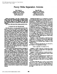
Figure 1: A lattice with 4 contexts and 5 axioms assigned to it
Definition 2.3 (Join prime). Let (L, N≤) be a lattice. Given a finite set K ⊆ L, let K⊗ := { ℓ∈M ℓ | M ⊆ K} denote the closure of K under the meet operator. An element ℓ ∈ L is called L join prime relative to K if, for every K ′ ⊆ K⊗ , ℓ ≤ k∈K ′ k implies that there is an k0 ∈ K ′ such that ℓ ≤ k0 .
1. ℓ ≤ λO≥ℓ , 2. S ⊆ O≥λS , and 3. O≥ℓ = O≥λO≥ℓ .
For instance, the lattice (L, ≤) depicted in Figure 1 has four join prime elements relative to L, namely ℓ0 , ℓ2 , ℓ3 , and ℓ5 . The element ℓ4 is not join prime relative to L since ℓ4 ≤ ℓ4 = ℓ5 ⊕ ℓ3 , but ℓ4 6≤ ℓ5 and ℓ4 6≤ ℓ3 . We now explain how lattices can be used to encode contexts, and solve reasoning problems relative to them. From our running example, we want to produce an access control system that regulates the allowed permissions for each user according to her user role. Our example focuses on reading access only. A common representation of user roles and their permissions to access objects is the access control matrix [18]. Using methods from Formal Concept Analysis, as presented in [19], a lattice representation of the access control matrix can be obtained. In fact, the lattice depicted in Figure 1 was derived in this way. In the general setting, we will use elements of the lattice (L, ≤) to define different contexts or views of an ontology. Depending on the application in hand, these contexts can have different meanings, such as access rights, level of expertise, trustworthiness, etc. Given an ontology O, every axiom a ∈ O is assigned a label lab(a) ∈ L, which intuitively expresses the contexts from which the axiom a can be accessed. An ontology extended with such a labelling function lab will be called a labelled ontology. We will use the expression Llab to denote the set of all labels occurring in the labelled ontology O; that is, Llab := {lab(a) | a ∈ O}. Each element ℓ ∈ L then defines the context sub-ontology4
Proof. For the first statement, byNdefinition ℓ ≤ lab(a) holds for all a ∈ O≥ℓ . Thus, ℓ ≤ a∈O≥ℓ lab(a) = λO≥ℓ . Regarding N the second claim, for every a ∈ S it holds that λS = s∈S lab(s) ≤ lab(a), which implies that a ∈ O≥λS . Now, consider the last claim. First, as ℓ ≤ λO≥ℓ , it holds trivially that O≥λO≥ℓ ⊆ O≥ℓ . From the second claim it also follows that O≥ℓ ⊆ O≥λO≥ℓ .
O≥ℓ := {a ∈ O | lab(a) ≥ ℓ}.
Just as every axiom is accessible only for certain contexts, a consequence of the ontology will only be derivable in those contexts that have access to enough axioms to deduce it. We are interested in computing adequate labels (called boundaries) for such implicit consequences, which express, just as the labels of the axioms, which contexts are capable of deducing them from their visible axioms. Notice that, if a consequence c follows from O≥ℓ for some ℓ ∈ L, it must also follow from O≥ℓ′ for every ℓ′ ≤ ℓ, since then O≥ℓ ⊆ O≥ℓ′ . A maximal element of L that still entails the consequence will be called a margin for this consequence.
Example 2.5. Let (L, ≤) be the lattice shown in Figure 1, where elements ℓ0 , ℓ2 , ℓ3 , ℓ5 represent the different kinds of users (that is, contexts) that have access to an ontology. Let lab be the labelling function assigning to each axiom ai of the ontology O from Example 2.2 the label ℓi , as depicted also in Figure 1. The label ℓ3 defines the context of a development engineer for which the sub-ontology O≥ℓ3 = {a1 , a2 , a3 , a4 }, along with all its consequences, is visible. Notice that labels that are lower in the lattice define larger context sub-ontologies. In other words, a user assigned to a context sub-ontology lower in the lattice will have access to more axioms (and thus, consequences) than a user belonging to a context above her.
3. Pre-Computing Knowledge
Conversely, every sub-ontology S ⊆ O defines Nan element λS ∈ L, called the label of S, given by λS := a∈S lab(a). Some simple relationships between ontologies and their labels are stated in the following lemma. Lemma 2.4. Let (L, ≤) be a lattice, O an ontology, and lab : O → L. For every ℓ ∈ L and S ⊆ O, it holds that 4 To define this sub-ontology, an arbitrary partial order would suffice. However, the existence of suprema and infima will be important for the computation of a boundary of a consequence (see Section 4).
4
Context-Dependent
Implicit
iff |S| ≥ 1. It is easy to see that there is no element ν ∈ L that satisfies the condition described above. Indeed, if we choose ν ∈ {ℓ0 , ℓ3 , ℓ4 , ℓ5 }, then ℓ2 violates the condition, ′ as ℓ2 6≤ ν, but O≥ℓ = {b2 } |= c. Similarly, if we choose 2 ν = ℓ2 , then ℓ1 violates the condition. Finally, if ν = ℓ1 is chosen, then ℓ1 itself violates the condition: ℓ1 ≤ ν, but ′ O≥ℓ = ∅ 6|= c. 1
Definition 3.1 (Margin). Let c be a consequence that follows from the ontology O. The label µ ∈ L is called a (O, c)-margin if O≥µ |= c, and for every ℓ with µ < ℓ we have O≥ℓ 6|= c. If O and c are clear from the context, we usually ignore the prefix (O, c) and call µ simply a margin. The following lemma shows three basic properties of the set of margins, which will be useful throughout this paper.
It is nonetheless possible to find an element that satisfies a restricted version of the condition, where we do not impose that the property (i.e. O≥ℓ |= c iff ℓ ≤ ν) must hold for every element of the context lattice, but only for those elements that are join prime relative to the labels of the axioms in the ontology.
Lemma 3.2. Let c be a consequence that follows from the ontology O. We have: 1. If µ is a margin, then µ = λO≥µ ; 2. if O≥ℓ |= c, then there is a margin µ such that ℓ ≤ µ; 3. there are at most 2|O| margins for c.
Definition 3.4 (Boundary). Let O be an ontology and c a consequence. An element ν ∈ L is called a (O, c)-boundary if for every element ℓ ∈ L that is join prime relative to Llab it holds that ℓ ≤ ν iff O≥ℓ |= c.
Proof. To show 1, let µ ∈ L. Lemma 2.4 yields µ ≤ λO≥µ and O≥µ = O≥λO≥µ , and thus O≥λO≥µ |= c. If µ < λO≥µ , then this λO≥µ contradicts our assumption that µ is a margin; hence µ = λO≥µ . Point 3 is a trivial consequence of 1: since every margin has to be of the form λS for some S ⊆ O, there are at most as many margins as there are subsets of O. For the remaining point, let ℓ ∈ L be such that O≥ℓ |= c. Let m := λO≥ℓ . From Lemma 2.4, it follows that ℓ ≤ m and O≥m = O≥ℓ , and hence O≥m |= c. If m is a margin, then the result holds; suppose to the contrary that m is not a margin. Then, there must exist an ℓ1 , m < ℓ1 , such that O≥ℓ1 |= c. As m = λO≥m , there must exist an axiom a ∈ O such that m ≤ lab(a), but ℓ1 6≤ lab(a). In fact, if m ≤ lab(a) ⇒ ℓ1 ≤ lab(a) N would hold for all a ∈ O, then m = λO≥ℓ = λO≥m = lab(a)≥m lab(a) ≥ ℓ1 , contradicting our choice of ℓ1 . The existence of this axiom a implies that O≥ℓ1 ⊂ O≥m . Let m1 := λO≥ℓ1 ; then m < ℓ1 ≤ m1 . If m1 is not a margin, then we can repeat the same process to obtain a new m2 with m < m1 < m2 and O≥m ⊃ O≥m1 ⊃ O≥m2 , and so on. As O is finite, there exists a finite k where this process stops, and hence mk is a margin.
As with margins, if O and c are clear from the context, we will simply call such a ν a boundary. When it is clear that the computed boundary and no assigned label is meant, we also often call it consequence label. In Example 3.3, the element ℓ1 is a boundary. Indeed, every join prime element ℓ relative to {ℓ4 , ℓ2 } (i.e., every element of ′ |= c. L except for ℓ1 ) is such that ℓ < ℓ1 and O≥ℓ From a practical point of view, our definition of a boundary has the following implication: we must enforce that contexts are always defined through labels that are join prime relative to the set Llab of all labels occurring in the ontology. In Example 2.5, all the elements of the context lattice except ℓ1 and ℓ4 are join prime relative to Llab and for this reason ℓ0 , ℓ2 , ℓ3 , ℓ5 are all valid context labels and can thus be used to represent user roles as illustrated. Given a context label ℓu , we will say that a consequence c is in the context if ℓu ≤ ν for some boundary ν. Notice however that the boundary is not guaranteed to be unique, as shown in the following example.
If we know that µ is a margin for the consequence c, then we know whether c follows from O≥ℓ for all ℓ ∈ L that are comparable with µ: if ℓ ≤ µ, then c follows from O≥ℓ , and if ℓ > µ, then c does not follow from O≥ℓ . However, this gives us no information regarding elements that are incomparable with µ. In order to obtain a full picture of when the consequence c follows from O≥ℓ for an arbitrary element ℓ of L, we can try to strengthen the notion of margin to that of an element ν of L that accurately divides the lattice into those elements whose associated sub-ontology entails c and those for which this is not the case, i.e., ν should satisfy the following: for every ℓ ∈ L, O≥ℓ |= c iff ℓ ≤ ν. Unfortunately, such an element need not always exist, as demonstrated by the following example.
Example 3.5. Consider the lattice L obtained from the lattice in Figure 1 by removing the element ℓ4 and keeping the order relation unchanged. Let now O = {a1 , a2 } and c be such that S |= c iff a1 ∈ S. If we set lab(a1 ) = ℓ3 , lab(a2 ) = ℓ5 , it then follows that (i) ℓ0 , ℓ3 , ℓ5 are all joinprime elements relative to Llab , and (ii) O≥ℓ |= c iff ℓ ≤ ℓ3 . But notice that ℓ3 ≤ ℓ2 and ℓ5 6≤ ℓ2 ; thus, ℓ2 and ℓ3 are both (O, c)-boundaries. Before formally describing how to compute (Section 4) and correct (Section 5) boundaries for consequences of an ontology, we briefly describe what are the requirements and benefits of our method from a knowledge engineering point of view. As a prerequisite, we assume that the context lattice L is known, and that every axiom of the ontology is labelled with an element of L expressing the set of contexts that have access to it. To obtain this lattice and labeling, the
Example 3.3. Consider the lattice (L, ≤) depicted in Figure 1 and let O’ be an ontology consisting of axioms b1 and b2 , labelled with ℓ4 and ℓ2 , respectively. Let now c be a consequence such that, for every S ⊆ O′ , we have S |= c 5
have boundaries different from the one of Lemma 4.1. To identify the particular boundary of Lemma 4.1, we will call it the margin-based boundary. For the rest of this section, we will focus on computing this boundary.
knowledge engineer can first build a context matrix relating every relevant context to the sub-ontology that it can access. The knowledge engineer only needs to “tag” every axiom with the corresponding contexts; tagging elements is already a common task in Web 2.0 applications, and no further effort is required from our framework. Formal Concept Analysis [20] can then be used to obtain a lattice representation of this matrix, together with a labelling function. This labelling function is ensured to be the least restrictive possible satisfying all the restrictions specified by the knowledge engineer in the context matrix. Indeed, the context lattice depicted in Figure 1 was derived in this way [19]. Given a labelled ontology, computing a boundary corresponds to reasoning with respect to all contexts simultaneously, modulo an inexpensive label comparison: given a boundary ν for a consequence c, every context below ν in the lattice can derive c, while all others cannot. Boundaries also simplify the work of verifying the correctness of the labelling function, since the knowledge engineer needs only compare the boundary of implicit consequences with the set of contexts that should access them, rather than analysing every context independently. If a consequence has an undesired boundary, then our method provides suggestions for correcting it, while keeping the changes in the labelling function to the minimum. In the same manner, our approach is helpful for the maintenance of labelled ontologies.
4.1. Using Full Axiom Pinpointing From Lemma 4.1 we know that the set of all margins yields sufficient information for computing a boundary. The question is thus how to compute this set. We now show that every margin can be obtained from some MinA. Lemma 4.2. For every margin µ for c there is a MinA S such that µ = λS . Proof. If µ is a margin, then O≥µ |= c by definition. Thus, there exists a MinA S ⊆ O≥µ . Since µ ≤ lab(a) for every a ∈ O≥µ , this in particular holds also for every axiom in S, and hence µ ≤ λS . Additionally, as S ⊆ O≥λS , we have O≥λS |= c. This implies µ = λS since otherwise µ < λS , and then µ would not be a margin. Notice that this lemma does not imply that the label of any MinA S corresponds to a margin. Indeed, for the ontology and consequence of Example 2.5, two of the four MinAs are {a1 , a2 , a5 }, {a1 , a2 , a4 } whose labels are ℓ0 and ℓ3 , respectively, and hence the label of the former cannot be a margin (since ℓ0 < ℓ3 ). However, as the consequence follows from every MinA S, Point 2 of Lemma 3.2 shows that λS ≤ µ for some margin µ. The following theorem is an immediate consequence of this fact together with Lemma 4.1 and Lemma 4.2.
4. Computing a Boundary
Theorem Ln 4.3. If S1 , . . . , Sn are all MinAs for O and c, then i=1 λSi is the margin-based boundary for c.
We now focus on the problem of computing a boundary. We first present an algorithm based on axiom-pinpointing, which introduces the main ideas for the computation of a boundary. We then improve on these ideas by taking the labels of the axioms into account during the computation. Finally, we show that, if the lattice is a total order, then a modification of binary search can be used to compute a boundary. All these algorithms are based on the following lemma.
Example 4.4. We continue Example 2.5 where each axiom ai is labelled with lab(ai ) = ℓi . We are interested in the boundary for the consequence SPrIncr (ecoCalc), which has the MinAs {a1 , a2 , a4 }, {a1 , a2 , a5 }, {a1 , a3 , a4 }, and {a1 , a3 , a5 }. From Theorem 4.3, it follows that the margin-based boundary for c is ℓ3 ⊕ ℓ0 ⊕ ℓ3 ⊕ ℓ0 = ℓ3 . This in particular shows that only the contexts of development engineers and customer service employees, defined through the labels ℓ3 and ℓ0 , respectively, can derive the consequence.
Lemma 4.1. Let µ1 , . . . , µn be all (O, c)-margins. Then Ln i=1 µi is a boundary for O, c.
Proof. Let ℓ ∈ L be Lnjoin prime relative to Llab . We need to show that ℓ ≤ i=1 µi iff O≥ℓ |= c. Assume first that O≥ℓ |= c. Then, from 2 of Lemma 3.2, it followsL that there n is a margin µj such that ℓ ≤ µ , and thus ℓ ≤ j i=1 µi . Ln Conversely, let ℓ ≤ i=1 µi . From 1 of Lemma 3.2, it follows that µi ∈ (Llab )⊗ for every i, 1 ≤ i ≤ n. As ℓ is join prime relative to Llab , it then holds that there is a j such that ℓ ≤ µj and hence, by the definition of a margin and the monotonicity of the consequence relation, O≥ℓ |= c.
According to the above theorem, to compute a boundary, it is sufficient to compute all MinAs. Several methods exist for computing the set of all MinAs, either directly [4, 11, 21] or through a so-called pinpointing formula [22, 8, 7], which is a monotone Boolean formula encoding all the MinAs. The main advantage of using the pinpointing-based approach for computing a boundary is that one can simply use existing implementations for computing all MinAs, such as the ones offered by the ontology editor Prot´eg´e 45 and the CEL system.6 However, since not
By Lemma 3.2, a consequence always has finitely many margins, and thus Lemma 4.1 shows that a boundary always exists. As shown in Example 3.5, a consequence may
5 http://protege.stanford.edu/ 6 http://code.google.com/p/cel/
6
Algorithm 1 Compute a MinLab of one MinA Procedure min-lab(O, c) Input: O: ontology; c: consequence Output: ML ⊆ L: a MinLab 1: if O 6|= c then 2: return no MinA 3: S := O 4: ML := ∅ 5: for every k ∈ Llab do N 6: if l∈ML l 6≤ k then 7: if S6=k |= c then 8: S := S6=k 9: else 10: ML := (ML \ {l | k < l}) ∪ {k} 11: return ML
all MinAs may really contribute to computing the boundary, first computing all MinAs may require extensive superfluous work. 4.2. Using Label-Optimized Axiom Pinpointing From Lemma 4.2 we know that every margin is of the form λS for some MinA S. In the previous subsection we have used this fact to compute a boundary by first obtaining the MinAs and then computing their labels. However, this idea ignores that the relevant part of the computation of a boundary are the labels of the MinAs, rather than the MinAs per se. This process can be optimized if we directly compute the labels of the MinAs, without necessarily computing the actual MinAs. Additionally, it is not necessary to compute the label of every MinA, but only of those that correspond to margins, that is, those that are maximal w.r.t. the lattice ordering ≤. For instance, in Example 4.4, we could avoid computing the two MinAs that have label ℓ0 . We present here a black-box algorithm that uses the labels of the axioms to find the boundary in an optimized way. Our algorithm is a variant of the Hitting-Set-Treebased [23] method (HST approach) for axiom pinpointing [11, 12]. First, we briefly describe the HST approach for computing all MinAs, which will serve as a starting point for our modified version. The HST-based method for axiom pinpointing computes one MinA at a time while building a tree that expresses the distinct possibilities to be explored in the search of further MinAs. It first computes an arbitrary MinA S0 for O, which is used to label the root of the tree. Then, for every axiom a in S0 , a successor node is created. If O \ {a} does not entail the consequence, then this node is a dead end. Otherwise, O \ {a} still entails the consequence. In this case, a MinA S1 for O \ {a} is computed and used to label the node. The MinA S1 for O \ {a} obtained this way is also a MinA of O, and it is guaranteed to be distinct from S0 since a ∈ / S1 . Then, for each axiom a′ in S1 , a new successor is created, and treated in the same way as the successors of the root node, i.e., it is checked whether O \ {a, a′ } still has the consequence, etc. This process obviously terminates since O is a finite set of axioms, and the end result is a tree, where each node that is not a dead end is labelled with a MinA, and every existing MinA appears as the label of at least one node of the tree (see [11, 12] for further details). An important ingredient of the HST algorithm is a procedure that computes a single MinA from an ontology. Such a procedure can, e.g., be obtained by going through the axioms of the ontology in an arbitrary order, and removing redundant axioms, i.e., ones such that the ontology obtained by removing this axiom from the current subontology still entails the consequence (see [21] for a description of this and of a more sophisticated logarithmic procedure for computing one MinA). We will use this same idea as a basis for computing the margin-based boundary for a consequence. As said before,
we are now not interested in actually computing a MinA, but only its label. This allows us to remove all axioms having a “redundant” label rather than a single axiom. Algorithm 1 describes a black-box method for computing the label of some MinA S based on this idea. More precisely, the algorithm does not compute a single label, but rather a minimal label set (MinLab) of a MinA S. Definition 4.5 (Minimal label set). Let S be a MinA for c. A set K ⊆ {lab(a) | a ∈ S} is called a MinLab of S ifNthe elements of K are pairwise incomparable and λS = ℓ∈K ℓ.
Algorithm 1 removes all the labels that do not contribute to a MinLab. If O is an ontology and ℓ ∈ L, then the expression O6=ℓ appearing at Line 7 denotes the sub-ontology O6=ℓ := {a ∈ O | lab(a) 6= ℓ}. If, after removing all the axioms labelled with k, the consequence still follows, then there is a MinA none of whose axioms is labelled with k. In particular, this MinA has a MinLab not containing k; thus, all the axioms labelled with k can be removed in our search for a MinLab. If the axioms labelled with k cannot be removed, then all MinAs of the current sub-ontology need an axiom labelled with k, and hence k is stored in the set ML . This set is also used to avoid useless N consequence tests: if a label is greater than or equal to ℓ∈ML ℓ, then the presence or absence of axioms with this label will not influence the final result, which will be given by the infimum of ML ; hence, there is no need to apply the (possibly complex) decision procedure for the consequence relation (Line 6). Theorem 4.6. Let O and c be such that O |= c. There is a MinA S0 for c such that Algorithm 1 outputs a MinLab of S0 . Proof. As O |= c, the algorithm will enter the for loop. This loop keeps the following two invariants: (i) S |= c and (ii) for every ℓ ∈ ML , S6=ℓ 6|= c. The invariant (i) is ensured by the condition in Line 7 that must be satisfied before S is modified. Otherwise, that is, if S6=ℓ 6|= c, then ℓ
7
Algorithm 2 Compute a boundary by a HST algorithm Procedure HST-boundary(O, c) Input: O: ontology; c: consequence Output: boundary ν for c 1: Global : C, H := ∅; ν 2: M := min-lab(O, c) 3: C := {M} N 4: ν := ℓ∈M ℓ 5: for each label ℓ ∈ M do 6: expand-HST(O6≤ℓ , c, {ℓ}) 7: return ν
is added to ML (Line 10) which, together with the fact that S is always modified to a smaller set (Line 8), ensures (ii). Hence, when the loop finishes, the sets S and ML satisfy both invariants. As S |= c, there is a MinA S0 ⊆ S for c. For each ℓ ∈ ML , there must be an axiom a ∈ S0 such that lab(a) = ℓ, otherwise, S0 ⊆ S6=ℓ and hence S6=ℓ |= c, which contradicts invariant (ii); Nthus, ML ⊆ {lab(a) | a ∈ S0 } and in particular λS0 ≤ ℓ∈ML ℓ. It remains to show that the inequality in the other direction holds as well. Consider now k ∈ {lab(a) | a ∈ S} and let MLk be the value of ML when N was enN the for loop tered with value k. We have that ℓ∈ML ℓ ≤ ℓ∈M k ℓ. If L N N k ℓ 6≤ k, and thus it fulfills ℓ∈ML ℓ 6≤ k, then also ℓ∈ML the test in Line 6, and continues to Line 7. If that test is satisfied, then all the axioms with label k are removed from S, contradicting the assumption that k = lab(a) for some a ∈ S. Otherwise,N k is added to ML , which contradicts the assumption that ℓ∈ML ℓ 6≤ k.NThus, for every axiom a N in S, ℓ∈ML ℓ ≤ lab(a); hence ℓ∈ML ℓ ≤ λS ≤ λS0 .
Procedure expand-HST(O, c, H) Input: O: ontology; c: consequence; H: list of lattice elements Side effects: modifies C, H, ν 1: if there exists some H ′ ∈ H such that {h ∈ H ′ | h 6≤ ν} ⊆ H or H ′ contains a prefix-path P with {h ∈ P | h 6≤ ν} = H then 2: return (early path termination ⊗) 3: if there exists M ∈ C such that for all ℓ ∈ M, h ∈ H, ℓ 6≤ h and ℓ 6≤ ν then 4: M′ := M (MinLab reuse) 5: else 6: M′ := min-lab(O6≤ν , c) 7: if O6≤ν |= c then ′ 8: C :=L C ∪ {M N } 9: ν := {ν, ℓ∈M′ ℓ} 10: for each label ℓ ∈ M′ do 11: expand-HST(O6≤ℓ , c, H ∪ {ℓ}) 12: else 13: H := H ∪ {H} (normal termination ⊙)
Once the label of a MinA has been found, we can compute new MinLabs by a successive deletion of axioms from the ontology using the HST approach. Suppose that we have computed a MinLab M0 , and that ℓ ∈ M0 . If we remove all the axioms in the ontology labelled with ℓ, and compute a new MinLab M1 of a MinA of this sub-ontology, then M1 does not contain ℓ, and thus M0 6= M1 . By iterating this procedure, we could compute all MinLabs, and hence the labels of all MinAs. However, since our goal is to compute the supremum of these labels, the algorithm can be further optimized by avoiding the computation of those MinAs whose labels will have no impact on the final result. Based on this we can actually do better than just removing the axioms with label ℓ: instead, all axioms with labels ≤ ℓ can be removed. For an element ℓ ∈ L and an ontology O, O6≤ℓ denotes the subontology obtained from O by removing all axioms whose labels are ≤ ℓ. Now, assume that we have computed the MinLab M0 , and that M1 6= M0 is the MinLab of the MinA S1 . For all ℓ ∈ M0 , if S1 is not contained in O6≤ℓ , then S1 contains an axiom N N with label ≤ ℓ. Consequently, m∈M1 m = λS1 ≤ m∈M0 m, and thus M1 need not be computed. Algorithm 2 describes our method for computing the boundary using a variant of the HST algorithm that is based on this idea. In the procedure HST-boundary, three global variables are declared: C, H (initialized with ∅), and ν. The variable C stores all the MinLabs computed so far, while each element of H is a set of labels such that, when all the axioms with a label less than or equal to any label from the set are removed from the ontology, the consequence does not follow anymore; the variable ν stores the supremum of the labels of all the elements in C and ultimately corresponds to the boundary that the method computes. The algorithm starts by computing a first MinLab M, which is used to label the root of a tree. For each element of M, a branch is created by calling the procedure expand-HST.
The procedure expand-HST implements the ideas of HST construction for computing all MinAs [11, 12] with additional optimizations that help reduce the search space as well as the number of calls to min-lab. First notice that each M ∈ C is a MinLab, and hence the infimum of its elements corresponds to the label of some MinA for c. Thus, ν is the supremum of the labels of a set of MinAs for c. If this is not yet the boundary, then there must exist another MinA S whose label is not less than or equal to ν. This in particular means that no element of S may have a label less than or equal to ν, as the label of S is the infimum of the labels of the axioms in it. When searching for this new MinA we can then exclude all axioms having a label ≤ ν, as done in Line 6 of expand-HST. Every time we expand a node, we extend the set H, which stores the labels that have been removed on the path in the tree to reach the current node. If we reach normal termination, it means that the consequence does not follow anymore from the reduced ontology. Thus, any H stored in H is such that, if all the axioms having a label less than or equal to an element in H are removed from O, then c does not follow anymore. Lines 1 to 4 of expand-HST are used to reduce the number of calls to the subroutine min-lab and the total 8
search space. We describe them now in more detail. The first optimization, early path termination, prunes the tree once we know that no new information can be obtained from further expansion. There are two conditions that trigger this optimization. The first one tries to decide whether O6≤ν |= c without executing the decision procedure. As said before, we know that for each H ′ ∈ H, if all labels less than or equal to any in H ′ are removed, then the consequence does not follow. Hence, if the current list of removal labels H contains a set H ′ ∈ H we know that enough labels have been removed to make sure that the consequence does not follow. It is actually enough to test whether {h ∈ H ′ | h 6≤ ν} ⊆ H since the consequence test we need to perform is whether O6≤ν |= c. The second condition for early path termination asks for a prefix-path P of H ′ such that P = H. If we consider H ′ as a list of elements, then a prefix-path is obtained by removing a final portion of this list. The idea is that, if at some point we have noticed that we have removed the same axioms as in a previous branch of the search, we know that all possibilities that arise from that search have already been tested before, and hence it is unnecessary to repeat the work. The tree can then be pruned at this node. As an example, consider a subtree reachable from the root by going along the edges ℓ1 , ℓ2 which has been expanded completely. Then all Hitting Sets of its leaf nodes share the common prefix-path P = {ℓ1 , ℓ2 }. Now suppose the tree is expanded by expand-HST(O, c, H) with H = {ℓ2 , ℓ1 }. The expansion stops with early termination since P = H. The second optimization avoids a possibly expensive call to min-lab by reusing a previously computed minimal label set. Notice that our only requirement on min-lab is that it produces a MinLab. Hence, any MinLab for the ontology obtained after removing all labels less than or equal to any h ∈ H or to ν would work. The MinLab-reuse optimization checks whether there is such a previously computed MinLab. If this is the case, the algorithm uses this set instead of computing a new one by calling min-lab. If we left out the prefix-path condition for early termination, the MinLab reuse condition would still hold. That means leaving out the prefix-path condition leads to no more minlab calls but leads to copying several branches in the tree without obtaining new information. Before showing that the algorithm is correct, we illustrate its execution through a small example.
Figure 2: An expansion of the HST method
test then whether O6=ℓ3 |= c and receive a negative answer; thus, ℓ3 is added to ML ; additionally, since ℓ3 < ℓ1 , the latter is removed from ML . Finally, O6=ℓ5 6|= c, and so we obtain ML = {ℓ3 , ℓ5 } as an output of min-lab. The MinLab {ℓ3 , ℓ5 }, is used as the root node n0 , setting the value of ν = ℓ3 ⊗ ℓ5 = ℓ0 . We then create the first branch on the left by removing all the axioms with a label ≤ ℓ3 , which is only a3 , and computing a new MinLab. Assume, for the sake of the example, that min-lab returns the MinLab {ℓ2 , ℓ4 }, and ν is accordingly changed to ℓ3 . When we expand the tree from this node, by removing all the axioms below ℓ2 (left branch) or ℓ4 (right branch), the instance relation c does not follow any more, and hence we have a normal termination, adding the sets {ℓ3 , ℓ2 } and {ℓ3 , ℓ4 } to H. We then create the second branch from the root, by removing the elements below ℓ5 . We see that the previously computed minimal label set of node n1 works also as a MinLab in this case, and hence it can be reused (MinLab reuse), represented in the figure as an underlined set. The algorithm continues now by calling expandHST(O6≤ℓ2 , c, {ℓ5 , ℓ2 }). At this point, we detect that there is H ′ = {ℓ3 , ℓ2 } satisfying the first condition of early path termination (recall that ν = ℓ3 ), and hence the expansion of that branch stops at that point. Analogously, we obtain an early path termination on the second expansion branch of the node n4 . The algorithm then outputs ν = ℓ3 , which is the margin-based boundary as computed before. Theorem 4.8. Let O and c be such that O |= c. Then Algorithm 2 computes the margin-based boundary of c. Proof. Let η be the margin-based boundary which, by Lemma 4.1, must exist. Notice first that the procedure expand-HST keeps as invariant that ν ≤ η as whenever ν is modified, it is only to join it with the infimum of a MinLab (Line 9), which by definition is the label of a MinA and, by Theorem 4.3, is ≤ η. Thus, when the algorithm terminates, we have that ν ≤ η. Assume now that ν 6= η. Then, there must exist a MinA S such that λS 6≤ ν; in particular, this implies that none of the axioms in S has a label ≤ ν and thus S ⊆ O6≤ν . Let M0 be the MinLab obtained in Line 2 of HST-boundary. There must then N be a h0 ∈ M0 such that S ⊆ O6≤h0 ; otherwise, λS ≤ ℓ∈M0 ℓ ≤ ν. There will then be a call to the process expand-HST with parameters O6≤h0 , c, and {h0 }. Suppose first that early path termination is not triggered. A MinLab M1 is then obtained, either by MinLab reuse
Example 4.7. We continue Example 4.4 with the same consequence SPrIncr (ecoCalc). Figure 2 shows a possible run of the HST-boundary algorithm. The algorithm first calls the routine min-lab(O, c). Consider that the for loop of min-lab is executed using the labels in the order ℓ1 , ℓ2 , ℓ4 , ℓ3 , ℓ5 since Line 5 requires no specific order. Thus, we try first to remove a1 labelled with ℓ1 . We see that O6=ℓ1 6|= c; hence a1 is not removed from O, and ML is updated to ML = {ℓ1 }. We then see that O6=ℓ2 |= c, and thus a2 is removed from O. Again, O6=ℓ4 |= c, so a4 is removed from O. At this point, O = {a1 , a3 , a5 }. We 9
Algorithm 3 Compute a boundary by binary search. Input: O: ontology; c: consequence Output: ν: (O, c)-boundary 1: if O 6|= c then 2: return no boundary 3: ℓ := 0lab ; h := 1lab 4: while l < h do 5: set m, ℓ < m ≤ h, such that |δ(ℓ, m) − δ(m, h)| ≤ 1 6: if O≥m |= c then 7: ℓ := m 8: else 9: h := pred(m) 10: return ν := ℓ
(Line 4) or by a call to min-lab (Line 6). As before, there is a h1 ∈ M1 with S ⊆ (O6≤h0 )6≤h1 . Additionally, since O6≤h0 does not contain any axiom labelled with h0 , we know h0 ∈ / M1 . While iterating this algorithm, we can find a sequence of MinLabs M0 , M1 , . . . , Mn and labels h0 , h1 , . . . , hn such that (i) hi ∈ Mi , (ii) S ⊆ O6≤hi , and (iii) hi ∈ / Mj for all i, j, 1 ≤ i < j ≤ n. In particular, this means that the Mi s are all different, and since there are only finitely many MinLabs, this process must terminate. Let Mn be the last set found this way. Then, when expand-HST is called with R := (((O6≤h0 )6≤h1 )... )6≤hn , c and H = {h1 , . . . , hn }, no new MinLab is found. Suppose first that this is due to a normal termination. Then, R6≤ν 6|= c. But that contradicts the fact that S is a MinA for c since S ⊆ R6≤ν . Hence, it must have finished by early termination. Early termination can be triggered by two different causes. Suppose first that there is a H ′ ∈ H such that {h ∈ H ′ | h 6≤ ν} ⊆ H. Then it is also the case that, for every h ∈ H ′ and S ⊆ O6≤h the following holds: if h ∈ H, then R ⊆ O6≤h ; otherwise, h ≤ ν and hence O6≤ν ⊆ O6≤h . Let R′ := {a ∈ O | there is no h ∈ H ′ with lab(a) ≤ h}. As H ′ ∈ H, it was added after a normal termination; thus, c does not follow from R′6≤ν . As S ⊆ R6≤ν , we obtain once again a contradiction. The second cause for early path termination is the existence of a prefix-path P with {h ∈ P | h 6≤ ν} = H. This means that in a previously explored path we had concluded that R6≤ν |= c, and a new MinLab Mn+1 was found. As in the beginning of this proof, we can then compute sets Mn+1 , . . . , Mm and hn+1 , . . . , hm (n < m) such that S ⊆ O6≤hi for all i, 1 ≤ i ≤ m and the Mi s are all different. Hence this process terminates. As before, the cause of termination cannot be normal termination, nor the first condition for early path termination. Thus, there must exist a new H ′′ ∈ H that fulfills the second condition for early termination. As H is a finite set, and each of its elements is itself a finite list, this process also terminates. When that final point is reached, there are no further causes of termination that do not lead to a contradiction, which means that our original assumption that ν 6= η cannot be true. Hence, ν is the margin-based boundary of c.
finite total order. We need to show that ℓ ≤ µ iff O≥ℓ |= c. Obviously, ℓ ≤ µ implies O≥ℓ ⊇ O≥µ , and thus O≥µ |= c yields O≥ℓ |= c. Assume now that O≥ℓ |= c. Then the fact that µ is maximal with this property together with the fact that ≤ is a linear order implies ℓ ≤ µ. Thus, µ is a boundary. A direct way for computing the boundary in this restricted setting thus consists of testing, for every element in ℓ ∈ Llab , in order (either increasing or decreasing) whether O≥ℓ |= c until the desired maximal element is found. This process requires in the worst case n := |Llab | iterations. This can be improved using binary search, which requires a logarithmic number of steps measured in n. Algorithm 3 describes the binary search algorithm. In the description of the algorithm, the following abbreviations have been used: 0lab and 1lab represent the minimal and the maximal elements of Llab , respectively; for ℓ1 ≤ ℓ2 ∈ Llab , δ(ℓ1 , ℓ2 ) := |{ℓ′ ∈ Llab | ℓ1 < ℓ′ ≤ ℓ2 }| is the distance function in Llab and for a given ℓ ∈ Llab , pred(ℓ) is the maximal element ℓ′ ∈ Llab such that ℓ′ < ℓ. The variables ℓ and h are used to keep track of the relevant search space. At every iteration of the while loop, the boundary is between ℓ and h. At the beginning, these values are set to the minimum and maximum of Llab and are later modified as follows: we first find the middle element m of the search space; i.e., an element whose distance to ℓ differs by at most one from the distance to h. We then test whether O≥m |= c. If that is the case, we know that the boundary must be larger or equal to m, and hence the lower bound ℓ is updated to the value of m. Otherwise, we know that the boundary is strictly smaller than m as m itself cannot be one; hence, the higher bound h is updated to the maximal element of Llab that is smaller than m; i.e., pred(m). This process terminates when the search space has been reduced to a single point, which must be the boundary. We have thus shown methods to compute a boundary and different optimizations techniques that can be used to improve their efficiency, as will be later shown in Section 6 in an empirical evaluation. Once this boundary has been computed, the knowledge engineer may notice that the
4.3. Using Binary Search for Linear Ordering Assume now that the context lattice (L, ≤) is a linear order, i.e., for any two elements ℓ1 , ℓ2 of L either ℓ1 ≤ ℓ2 or ℓ2 ≤ ℓ1 . We show that in this case, the computation of the boundary can be further optimized through a variant of binary search. First, we give a characterization of the boundary in this setting. Lemma 4.9. Let O and c be such that O |= c. Then the unique boundary of c is the maximal element µ of Llab with O≥µ |= c. Proof. Let µ be the maximal element of Llab such that O≥µ |= c. Such a maximal element exists since Llab is a 10
consequence belongs to an unwanted set of contexts. In that case, she would like to change the labelling function to correct the contexts to which this consequence belongs. In the next section we will describe methods for finding minimal changes for obtaining the desired boundary.
L
L
L
ℓc
ℓc
ℓg
ℓg
Lg ℓc
Lc ℓg Lc
Lg
Lg
Lc
5. Repairing a Boundary Figure 3: Hide consequence from some contexts (left), allow additional contexts to see consequence (right), and both at the same time (middle)
Just as ontology development and maintenance is an error prone activity, so is the adequate labelling of axioms. Indeed, several seemingly harmless axioms might possibly be combined to deduce knowledge that is considered to be out of the scope of a context. On the other hand, an over-restrictive labelling of axioms may cause harmless or fundamental knowledge to be inaccessible to some contexts.
of minimum cardinality, or smallest CS for short, is obviously also a MinCS. However, the reverse is not necessarily true. A MinCS is minimal with respect to set inclusion but is not necessarily a smallest CS since there might be several MinCS of different cardinality. This is similar to the minimality of MinA (see Definition 2.1), where a MinA is also not necessarily a MinA of minimum cardinality. It follows from results in [22] that it is NP-complete to determine whether the cardinality of a smallest CS is equal to a given natural number, and thus smallest change sets cannot be computed in polynomial time (unless P=NP). Let ℓg denote the goal label and ℓc the margin-based boundary for c. If ℓg 6= ℓc , we have three cases which are illustrated in Figure 3: either (1) ℓg < ℓc (left), (2) ℓc < ℓg (right), or (3) ℓg and ℓc are incomparable (middle). In our example, where ℓc = ℓ3 , the three cases can be obtained by ℓg being ℓ0 , ℓ4 , and ℓ5 , respectively. The sets Lc and Lg contain the labels defining contexts that can respectively deduce the consequence before and after the label changes. Consider first the case where ℓc < ℓg . From Theorem 4.3 it follows that any MinA S is a change set for ℓg : since ℓc < ℓg , then for every MinA S ′ , it follows that λS ′ < ℓg . But then, under the new labelling labS,ℓg it follows that
Example 5.1. We continue Example 2.5. The ontology entails the consequence c = SPrIncr (ecoCalc) and the computed boundary of c is ℓ3 (see Example 4.4), which implies that only for contexts labelled with ℓ0 and ℓ3 , c is visible. That means the consequence c can only be seen by the development engineers and customer service employees (see Figure 1). It could be, however, that c is not expected to be accessible to customer service employees and development engineers, but rather to customer service employees and customers. In that case, we wish to modify the boundary of c to ℓ5 . If the knowledge engineer notices that the boundary for a given consequence differs from the desired one, then it would be helpful if she could use automatically generated suggestions for how to modify the labelling function in order to correct this error. This problem can be formalized and approached in several different ways. Here, we assume that the knowledge engineer knows the exact boundary ℓg that the consequence c should receive, and we try to find a set S of axioms of minimal cardinality such that, if all the axioms in S are relabelled to ℓg , then the boundary of c will be ℓg .
O a∈S
labS,ℓg (a) =
O
ℓg = ℓg ,
a∈S
and hence when the least upper bound of all the labels of all MinAs is computed, we obtain the boundary ℓg , as desired. For the case where ℓg < ℓc , we will use a similar argument as before, based on a result dual to the result in Theorem 4.3:
Definition 5.2 (Change set). Let O be an ontology, c a consequence, lab a labelling function, S ⊆ O and ℓg ∈ L the goal label. The modified assignment labS,ℓg is given by ( ℓg , if a ∈ S, labS,ℓg (a) := lab(a), otherwise.
Theorem Nn 5.3. L If S1 , . . . , Sn are all diagnoses for O,c, then i=1 ( a∈Si lab(a)) is a boundary for c.
Proof. Let first ℓ ∈ L be such that O≥ℓ |= c, and let Si , 1 ≤ i ≤ n be a diagnosis for O,c. Since O≥ℓ |= c, there must be an axiom a ∈ Si L such that a ∈ O≥ℓ . This means that lab(a) ≥ ℓ and hence a∈Si lab(a) ≥ ℓ. As this is true Nn L for each diagnosis, it holds that i=1 ( a∈Si lab(a)) ≥ ℓ. For the converse, let ℓ ∈ LNbe a L join prime element n relative to Llab such that ℓ ≤ i=1 ( a∈Si lab(a)). This in particular means that, for every diagnosis Si for O,c, L ℓ ≤ a∈Si lab(a). But since ℓ is join prime relative to Llab and for each a ∈ Si lab(a) is an element of Llab , it holds
A sub-ontology S ⊆ O is called a change set (CS) for ℓg if the boundary for O,c under the labelling function labS,ℓg equals ℓg . It is a minimal CS (MinCS) if the set is minimal (w.r.t. set inclusion) with this property. Obviously, the original ontology O is always a change set for any goal label if O |= c. However, we are interested in performing minimal changes to the labelling function. Hence, we search first for minimal change sets, and later for a change set of minimum cardinality. A change set 11
that there must exist some ai ∈ Si such that ℓ ≤ lab(ai ). Thus, O≥ℓ ∩ Si 6= ∅ for every i, 1 ≤ i ≤ n. Since S1 , . . . , Sn are all diagnoses for O,c, it follows that O≥ℓ |= c.
In the following, we will say that a set S is a minimal union of a RAS and an IAS if (i) there exist a RAS R and an IAS I such that S = R∪I and (ii) for every RAS R′ and IAS I ′ , R′ ∪ I ′ is not strictly contained in S. The following theorem justifies the use of IAS and RAS when searching for the minimal change sets and a smallest change set.
Notice that, due to the duality between MinAs and diagnoses, if the lattice L is distributive, then the boundary given by this theorem is the same as the margin-based boundary. From Theorem 5.3, it follows that, if ℓg < ℓc , then every diagnosis is a change set for ℓg . The third case can be addressed using a combination of the previous two approaches: if ℓg and ℓc are incomparable, we can first set as a partial goal ℓ′g = ℓg ⊗ ℓc . Thus, we can first apply the method dealing with the first case, to set the boundary to ℓ′g , and then, using the second approach, modify this new boundary once more to ℓg . Rather than actually performing this task as a two-step computation, we can simply compute a MinA and a diagnosis. The union of these two sets yields a CS. Unfortunately, the CS computed as described above is not necessarily a MinCS, even if a smallest diagnosis or a smallest MinA is used, as shown in the following example.
Theorem 5.6. Let ℓc be a boundary for O,c, ℓg the goal label, and S ⊆ O. Then, the following holds: • if ℓc < ℓg then S is a MinCS iff S is an IAS, • if ℓg < ℓc then S is a MinCS iff S is a RAS, • if ℓc and ℓg are incomparable then S is a MinCS iff S is a minimal union of a RAS and an IAS. Proof. We prove only the first result. The other two can be shown analogously. Let first S be a MinCS. From Theorem 4.3 it follows that S ⊆ O6≥ℓg since otherwise S would not be minimal. N Since S is a change set, there is a MinA S ′ such that a∈S ′ labS,ℓg (a) ≥ ℓg ; that is, labS,ℓg (a) ≥ ℓg for every a ∈ S ′ . This means that S ′ ⊆ O≥ℓ ∪ S and thus O≥ℓ ∪ S |= c. Hence S is an IAS. Conversely, let S be an IAS; then S is clearly also a change set. If it was not a MinCS, then there would exist an axiom a ∈ S such that S \ {a} is also a change set, but as shown before, this would imply that S \ {a} is an IAS, which violates the minimality condition.
Example 5.4. Let O,c and lab be as in Example 2.5 with the consequence SPrIncr (ecoCalc). We then know that ℓc := ℓ3 is a boundary for O,c. Suppose now that c shall remain visible for those who see it already and additionally made available to customers, i.e. the goal label is ℓg := ℓ4 . Since ℓc < ℓg , we know that any MinA is a change set. Since all MinAs for O,c have exactly three elements, any change set produced this way will have cardinality three. However, {a2 } is also a CS. More precisely it is a MinCS.
Obviously, this theorem also yields a direct approach for computing a CS of minimal cardinality. Corollary 5.7. Let ℓc be a boundary for O,c, and ℓg the goal label. Then a CS of minimal cardinality can be found by computing a RAS, an IAS and a union of an IAS and a RAS of minimal cardinality.
To understand why the minimality of MinAs is not sufficient for obtaining a MinCS, we can look back to Theorem 4.3. This theorem states that, in order to find a boundary, we need to compute the join of all λS , with S a MinA, and λS the meet of the labels of all axioms in S. But then, for any axiom a ∈ S such that ℓg ≤ lab(a), modifying this label to ℓg will have no influence on the result of λS . In Example 5.4, there is a MinA {a1 , a2 , a4 }, where two axioms, namely a1 and a4 have a label greater or equal to ℓg = ℓ4 . Thus, the only axiom that needs to be relabelled is in fact a2 , which yields the MinCS {a2 } shown in the example. Basically, we can consider every axiom a ∈ O such that ℓg ≤ lab(a) as fixed in the sense that it is superfluous for any change set. Analogously, one can view some of the axioms in a diagnosis as being fixed when trying to compute a change set for decreasing the boundary. For this reason, we will introduce generalizations of MinAs and diagnoses, which we call IAS and RAS, respectively.
The cardinality of a smallest union of an IAS and a RAS cannot be computed from the cardinalities of a smallest RAS and a smallest IAS since combining the smallest IAS and RAS does not necessarily yield a smallest CS. The following example illustrates this. Example 5.8. Assume {a1 , a2 }, {a2 , a3 } are the smallest RAS and {a1 , a4 } is the smallest IAS, then {a1 , a2 , a4 } is the smallest CS and has cardinality 3. However, combining a smallest IAS and a smallest RAS might yield a MinCS (but not a smallest CS) of cardinality 4. We now describe how to compute a smallest change set. As in the previous section, we first present the most obvious approach that is based on the computation of all MinAs and diagnoses. Afterwards, we show how this idea can be improved by considering fixed portions of the ontology and computing the set of IAS and RAS, as described before. These methods compute all minimal change sets, from which those with the smallest cardinality can be easily extracted. If one is only interested in a smallest CS, then we can further improve this approach showing that it
Definition 5.5 (IAS, RAS). A minimal inserted axiom set (IAS) for ℓg is a subset I ⊆ O6≥ℓg such that O≥ℓg ∪I |= c and for every I ′ ⊂ I : O≥ℓg ∪ I ′ 6|= c. A minimal removed axiom set (RAS) for ℓg is a subset R ⊆ O6≤ℓg such that O6≤ℓg \ R 6|= c and for every R′ ⊂ R : O6≤ℓg \ R′ |= c. 12
suffices to compute only partial MinCS by putting a cardinality limit, thus reducing the search space and execution time of our method. Although we have shown in Example 5.4 that MinAs and diagnoses do not yield MinCS or even smallest CS directly, both of these change sets can still be deduced from the set of all MinAs and diagnoses, as shown by the following lemma.
Algorithm 4 Compute a (partial) IAS Procedure extract-partial-IAS(Ofix , Otest , c, n) Input: Ofix : fixed axioms; Otest : axioms; c: consequence; n: limit Output: first n elements of a minimal S ⊆ Otest such that Ofix ∪ S |= c 1: Global l := 0, n 2: return extract-partial-IAS-r(Ofix , Otest , c) Subprocedure extract-partial-IAS-r(Ofix , Otest , c) 1: if n = l then 2: return ∅ 3: if |Otest | = 1 then 4: l := l + 1 5: return Otest 6: S1 , S2 := halve(Otest ) 7: if Ofix ∪ S1 |= c then 8: return extract-partial-IAS-r(Ofix , S1 , c) 9: if Ofix ∪ S2 |= c then 10: return extract-partial-IAS-r(Ofix , S2 , c) 11: S1′ := extract-partial-IAS-r(Ofix ∪ S2 , S1 , c) 12: S2′ := extract-partial-IAS-r(Ofix ∪ S1′ , S2 , c) 13: return S1′ ∪ S2′
Lemma 5.9. Let I (R) be an IAS (RAS) for ℓg , then there is a MinA (diagnosis) S such that I = S \ O≥ℓg (R = S \ O≤ℓg ). Proof. Let I be an IAS. Then O≥ℓg ∪ I |= c, and hence there is a MinA S ⊆ O≥ℓg ∪ I. As O≥ℓg ∩ I = ∅ it follows that I = S \ O≥ℓg . The case for RAS is analogous. Lemma 5.9 shows that we can compute the set of all IAS by first computing all MinAs and then removing the set of fixed elements O≥ℓg from it. Thus, the most na¨ıve approach for computing a change set of minimum cardinality is to first find all MinAs, then compute the set of all IAS by removing all elements in O≥ℓg , and finally search for the IAS having the least elements. The same procedure applies to RAS, using diagnoses instead of MinAs. As explained before, all MinAs can be computed using a HST-based algorithm. Although not stated explicitly in the axiom pinpointing literature, it is clear that the same HST algorithm can be used for computing all diagnoses. The only variant necessary is to have a subroutine capable of computing one such diagnosis, which can be obtained by dualizing the algorithm for computing one MinA (see Algorithms 4 and 5 for an example on how this dualization works). In our experiments, we used this approach as a basis to measure the improvement achieved by the optimizations that will be introduced next. Na¨ıvely a CS with the lowest cardinality can be found by computing all MinCS and selecting one of minimal size. To find all MinCS, we can use a HST algorithm that uses an auxiliary procedure that computes a single MinCS. For this auxiliary procedure, we can use two subprocedures extracting RAS and IAS, respectively, as evidenced by Theorem 5.6. We now describe an approach for computing a smallest CS directly, which again uses a variant of the HST algorithm. In Algorithm 4 we present a variation of the logarithmic MinA extraction procedure presented in [21] that is able to compute an IAS or stop once this has reached a size n, in which case it returns the partial IAS computed so far. In this algorithm, the auxiliary procedure halve partitions an ontology into two disjoint subsets of axioms whose difference in cardinality is at most 1. We also show the dual variant for computing a RAS in Algorithm 5. Given a goal label ℓg , if we want to compute an IAS or a partial IAS of size at most n for a consequence c, then we would make a call to extract-partial-IAS(O≥ℓg , O6≥ℓg , c, n). Similarly, a call to extract-partial-RAS(O6≤ℓg , O6≤ℓg , c, n) yields a RAS of size ≤ n or a partial RAS of size exactly
n. The cardinality limit will be used to avoid unnecessary computations when looking for a smallest CS. With the help of the procedures to extract RAS and IAS, Algorithm 6 describes how to compute a MinCS with a cardinality limit. In the first lines of this algorithm, lbl(c) expresses the margin-based boundary of the consequence c. In order to label a node, we compute a MinCS with extract-partial-MinCS(O, lab, c, ℓg , H, n), where H is the set of all labels attached to edges on the way from the node to the root of the tree. Note that all the axioms in H are removed from the search space to extract the new IAS and RAS. Furthermore, axioms in the IAS computed in Line 4 of this algorithm are considered as fixed for the RAS computation. The returned set is a MinCS of size ≤ n or a partial MinCS of size n. Example 5.10. Returning to our running example, suppose now that we want to hide c from development engineers and make it available to customers, i.e. modify the label of consequence c to ℓg = ℓ5 . Algorithm 6 starts by making a call to extract-partial-IAS(O≥ℓ5 , O6≥ℓ5 , c, ∞).7 A possible output for this call is I = {a3 }. We can then call extract-partial-RAS(O6≤ℓ5 \I, O6≤ℓ5 \I, c, ∞), which may output e.g. the set R = {a1 }. Thus, globally the algorithm returns {a3 , a1 }, which can be easily verified to be a MinCS for ℓ5 . One of the advantages of the HST algorithm is that the labels of any node are always ensured not to contain 7 For the sake of this example, we ignore the cardinality limit, as we want to describe only how one MinCS is computed.
13
Algorithm 5 Compute a (partial) RAS Procedure extract-partial-RAS(Ononfix , Otest , c, n) Input: Ononfix : axioms; Otest ⊆ Ononfix : axioms; c: consequence; n: limit Output: first n elements of a minimal S ⊆ Otest such that Ononfix \ S 6|= c 1: Global l := 0, Ononfix , n 2: return extract-partial-RAS-r(∅, Otest , c) Subprocedure extract-partial-RAS-r(Ohold , Otest , c) 1: if n = l then 2: return ∅ 3: if |Otest | = 1 then 4: l := l + 1 5: return Otest 6: S1 , S2 := halve(Otest ) 7: if Ononfix \ (Ohold ∪ S1 ) 6|= c then 8: return extract-partial-RAS-r(Ohold , S1 , c) 9: if Ononfix \ (Ohold ∪ S2 ) 6|= c then 10: return extract-partial-RAS-r(Ohold , S2 , c) 11: S1′ := extract-partial-RAS-r(Ohold ∪ S2 , S1 , c) 12: S2′ := extract-partial-RAS-r(Ohold ∪ S1′ , S2 , c) 13: return S1′ ∪ S2′
Algorithm 6 Compute a (partial) MinCS Procedure extract-partial-MinCS(O, lab, c, ℓg , H, n) 1: iI := ℓg 6< lbl(c) ∧ O≥ℓg 6|= c 2: iR := ℓg 6> lbl(c) ∧ O6≤ℓg |= c 3: return extract-partial-MinCS(O, lab, c, ℓg , iI , iR , H, n) Procedure extract-partial-MinCS(O, lab, c, ℓg , iI , iR , H, n) Input: O, lab: labelled ontology; c: consequence; ℓg : goal label; iI : decision to compute IAS; iR : decision to compute RAS; H: HST edge labels; n: limit Output: first n elements of a MinCS S ⊆ O 1: if iI ∧ O≥ℓg ∪ (O6≥ℓg \ H) 6|= c or iR ∧ H |= c then 2: return ∅ (HST normal termination) 3: if iI then 4: I := extract-partial-IAS(O≥ℓg , O6≥ℓg \ H, c, n) 5: if iR and O6≤ℓg \ I |= c then 6: R := extract-partial-RAS(O6≤ℓg \ I, O6≤ℓg \ (I ∪ H), c, n − |I|) 7: return I ∪ R
Proof. The described algorithm outputs a CS since the globally stored and finally returned S is only modified when the output of extract-partial-MinCS has size strictly smaller than the limit n, and hence only when this is indeed a CS itself. Suppose now that the output S is such that m < |S|, and let S0 be a MinCS such that |S0 | = m, which exists by assumption. Then, every set obtained by calls to extract-partial-MinCS has size strictly greater than m, since otherwise, S and n would be updated. Consider now an arbitrary set S ′ found during the execution through a call to extract-partial-MinCS, and let Sn′ := {a1 , . . . , an } be the first n elements of S ′ . Since S ′ is a (partial) MinCS, it must be the case that S0 6⊆ Sn′ since every returned MinCS is minimal in the sense that no axiom might be removed to obtain another MinCS. Then, there must be an i, 1 ≤ i ≤ n such that ai ∈ / S0 . But then, S0 will still be a MinCS after axiom {ai } has been removed. Since this argument is true for all nodes, it is in particular true for all leaf nodes, but then they should not be leaf nodes, since a new MinCS, namely S0 can still be found by expanding the HST, which contradicts the fact that S is the output of the algorithm.
the label of any of its predecessor nodes. In particular this means that even if we compute a partial MinCS, the algorithm will still correctly find all MinCS that do not contain any of the partial MinCS found during the execution. Since we are interested in finding the MinCS of minimum cardinality, we can set the limit n to the size of the smallest CS found so far. This limit is initially fixed to the size of the ontology. If extract-partial-MinCS outputs a set with fewer elements, we are sure that this is indeed a full MinCS, and our new smallest known CS. The HST algorithm will not find all MinCS in this way, but we can be sure that one MinCS with the minimum cardinality will be found. The idea of limiting the cardinality in order to find a smallest MinCS can be taken a step further by not expanding each node for all the axioms in it, but rather only on the first n − 1, where n is the size of the smallest CS found so far. This further reduces the search space by decreasing the branching factor of the search tree. Notice that the highest advantage of this second optimization appears when the HST is constructed in a depth-first fashion. In that case, a smaller MinCS found further below in the tree will reduce the branching factor of all its predecessors. Hence, the cardinality limit reduces the search space in two dimensions: (1) the computation of a single MinCS is limited to n axioms and (2) only n − 1 axioms are expanded from each node. Algorithm 7 is the resulting HST algorithm. The following theorem states that it is correct. Theorem with O |= cardinality CS S such
Example 5.12. Coming back to our running example, suppose that we want to hide c from development engineers, i.e. set the label of c to ℓg = ℓ0 . Algorithm 6 first calls extract-partial-RAS(O6≤ℓ0 , O6≤ℓ0 , c, 5). A possible output of this call is R = {a2 , a3 }. The tree now branches through a2 and a3 . In the first case it calls extract-partialRAS(O6≤ℓ0 , O6≤ℓ0 \ {a2 }, c, 2), which could yield the RAS R = {a4 , a5 }. This might be a partial MinCS since its size equals the cardinality limit. The next call extract-partialRAS(O6≤ℓ0 , O6≤ℓ0 \{a2 , a4 }, c, 2) yields a smallest R = {a1 }, and the HST terminates. Notice that if {a1 } had been the first MinCS found, the process would have immediately terminated.
5.11. Let O be an ontology, c a consequence c, and ℓg a goal label. If m is the minimum of all CS for ℓg , then Algorithm 7 outputs a that |S| = m. 14
Figure 4: Hitting Set Trees to compute all MinAs (left) and a smallest change set for ℓg = ℓ5 (right)
Algorithm 7 Compute a smallest CS by a HST algorithm Procedure HST-extract-smallest-CS(O, lab, (L, ≤), c, ℓg ) Input: O,lab: labelled ontology; (L, ≤): lattice; c: consequence; ℓg : goal boundary Output: a smallest CS S 1: Global C, H, S := O, n := |O|, c, isI := ℓg 6< lbl(c) ∧ O≥ℓg 6|= c; isR := ℓg 6> lbl(c) ∧ O6≤ℓg |= c 2: expand-HST-CS(∅) 3: return S
However, it should be clear that both, node-reuse and early path termination, can be included in the algorithm without destroying its correctness. The implementation used in our experiments applies these two optimizations. Example 5.13. We continue Example 2.5 with the same consequence SPrIncr (ecoCalc). For goal label ℓg = ℓ5 , Figure 4 shows the expansion of the HST trees computing all MinAs and all diagnoses (left), in comparison with the one obtained for computing a smallest change set using both optimizations: fixed axioms and cardinality limit (right). Obviously, the number of nodes, the node cardinality and the number of tree expansions is lower.
Procedure expand-HST-CS(H) Input: H: list of edge labels Side effects: modifications to C and H 1: if there exists some H ′ ∈ H such that H ′ ⊆ H or H ′ contains a prefix-path P with P = H then 2: return (early termination ⊗) 3: else if there exists some Q′ ∈ C such that H ∩ Q′ = ∅ then 4: Q := Q′ (MinCS reuse) 5: else 6: Q := extract-partial-MinCS(O, lab, c, ℓg , isI , isR , H, n) 7: if ∅ = Q then 8: H := H ∪ {H} (normal termination ⊙) 9: return 10: if |Q| < |S| then 11: n := |Q| 12: S := Q 13: C := C ∪ {Q} 14: for the first (n − 1) axioms a ∈ Q do 15: expand-HST-CS(H ∪ {a})
6. Empirical Evaluation On large real-world ontologies, we empirically evaluated implementations of the algorithms to (1) compute a boundary for a consequence and (2) repair this boundary if needed. The following sections describe the test data and the test environment first, and then present the empirical results, which show that our algorithms perform well in practical scenarios. 6.1. Test Data and Test Environment We performed our tests on a PC with 2GB RAM and Intel Core Duo CPU 3.16GHz. We implemented all approaches in Java 1.6 and for convenient OWL file format parsing and reasoner interaction we used the OWL API for OWL 2 [24] in trunk revision 1150 from 21.5.2009.8 6.1.1. Context Lattices Although we focus on comparing the efficiency of the presented algorithms, and not on practical applications of these algorithms, we have tried to use inputs that are closely related to ones encountered in applications. The two context lattices (Ld , ≤d ) and (Ll , ≤l ) are similar to ones encountered in real-world applications. The context lattice (Ld , ≤d ), already introduced in Figure 1, was developed and applied in an access policy scenario [19].
Efficient implementations of the original version of the HST algorithm rely on several optimizations. Two standard optimizations described in the literature are nodereuse and early path termination (see, e.g. [11, 12, 14]). Node-reuse keeps a history of all nodes computed so far in order to avoid useless (and usually expensive) calls to the auxiliary procedure that computes a new node. Early path termination, on the other hand, prunes the Hitting Set Tree by avoiding expanding nodes when no new information can be derived from further expansion. In order to avoid unnecessary confusion, we have described the modified HST algorithm without including these optimizations.
8 Subversion Repository https://owlapi.svn.sourceforge.net/ svnroot/owlapi/owl1_1/trunk
15
The context lattice (Ll , ≤l ) is a linear order with 6 elements Ll = Ld = {ℓ0 , . . . , ℓ5 } with the obvious ordering ≤l := {(ℓn , ℓn+1 ) | ℓn , ℓn+1 ∈ Ll ∧ 0 ≤ n ≤ 5}. This lattice could represent an order of trust values as in [25] or dates from a revision history, to name just two applications.
HST-extract-all-MinAs procedure (Algorithm 9 from [12]). The set of extracted MinAs is then used to calculate the label of the consequence. We stop the execution after 10 MinAs have been found in order to limit the runtime; thus, some of the labels found may not be the final result. The boundary computation with label-optimized axiom pinpointing (LP) with min-lab and HST-boundary are implementations of Algorithm 1 and Algorithm 2. The boundary computation with binary search for linear ordering (BS in the following) implements Algorithm 3. We tested 8 combinations resulting from the 2 ontologies OSnomed and OFunct , with the two approaches FP and LP over the lattice (Ld , ≤d ) and the two approaches LP and BS over the lattice (Ll , ≤l ).
6.1.2. Ontologies, Label Assignment and Reasoners We used the two ontologies OSnomed and OFunct with different expressivities and types of consequences for our experiments. The Systematized Nomenclature of Medicine, Clinical Terms (Snomed ct) is a comprehensive medical and clinical ontology which is built using the DL EL++ . Our version of OSnomed is the January/2005 release of the DL version, which contains 379,691 concept names, 62 object property names, and 379,704 axioms. Since more than five million subsumptions are consequences of OSnomed , testing all of them was not feasible and we used the same sample subset as described in [21], i.e., we sampled 0.5% of all concepts in each top-level category of OSnomed . For each sampled concept A, all subsumptions A ⊑ B following from OSnomed with A as subsumee were considered. Overall, this yielded 27,477 subsumptions. Following the ideas of [21], we pre-computed the reachability-based module for each sampled concept A with the reasoner CEL 1.0 [26] and stored these modules. The module for A is guaranteed to contain all axioms of any MinA and any diagnosis, thus also any IAS and RAS, for each subsumption A ⊑ B with A the considered subsumee. This module was then used as the start ontology when considering subsumptions with subsumee A, rather than using the complete ontology. The OWL ontology OFunct has been designed for functional descriptions of mechanical engineering solutions and was presented in [27, 28]. It has 115 concept names, 47 object property names, 16 data property names, 545 individual names, 3,176 axioms, and the DL expressivity used in the ontology is SHOIN (D). Its 716 consequences are 12 subsumption and 704 instance relationships (concept assertions). To obtain labelled ontologies, axioms in both ontologies received a random label assignment of elements from the set Ll = Ld . Our test suite provides a great variety of cases: consequences with many or few MinAs, with very large or very small MinAs, cases with a high or low boundary, etc. Hence, our results should not differ greatly if a different label assignment is used. As black-box subsumption and instance reasoner we used Pellet 2.0 [29], since it can deal with the expressivity of both ontologies. For the expressive DL SHOIN (D) it uses a tableau-based algorithm and for EL++ it uses an optimized classifier for the OWL 2 EL profile that is based on the algorithm described in [30].
6.1.4. Test Setting for Repairing a Boundary We tested repairing access restrictions to implicit knowledge in the following setting. We took the computed boundary ℓc of each consequence c of the ontologies from the first experiment and then computed the MinCS to reach the goal boundary ℓg which is constantly ℓ3 in all experiments. Consequences were not considered if ℓc = ℓg . Thus, from the 716 consequences in OFunct , we have 415 remaining with context lattice (Ld , ≤d ) and 474 remaining with (Ll , ≤l ). From the 27,477 consequences in OSnomed we have 23,695 remaining with context lattice (Ld , ≤d ) and 25,897 with (Ll , ≤l ). The MinCS computation with FP uses the procedures log-extract-MinA and the HST based HST-extract-all-MinAs, implemented by the algorithms mentioned above. The MinCS computation with extract-partial-MinCS and the smallest CS computation with HST-extract-smallest-CS including optimizations for fixed axioms and cardinality limit are implementations of Algorithm 6 and Algorithm 7. The required IAS and RAS extraction with extract-partial-IAS, extract-partial-RAS are implementations of Algorithms 4 and 5, respectively. We stop after 10 MinAs (or respectively MinCS or partial MinCS) have been found in order to limit the runtime; hence there might be no computed MinCS at all or a nonsmallest MinCS returned. We tested 12 combinations resulting from the two ontologies OSnomed and OFunct , two context lattices (Ld , ≤d ) and (Ll , ≤l ) and three algorithm variants (FP, fixed axioms, and fixed axioms in combination with cardinality limit). Running the fixed axioms optimization without cardinality limit can be done easily by skipping Line 11 in Algorithm 7. 6.2. Experimental Results Our experiments show that our algorithms perform well on practical large-scale ontologies. In the following we describe our empirical results for each of the two discussed tasks with labelled ontologies, i.e. computing a boundary to discover access restrictions to a given consequence and repair the boundary of a single consequence by changing axiom labels.
6.1.3. Test Setting for Computing a Boundary The boundary computation with full axiom pinpointing (FP) uses log-extract-MinA (Algorithm 2 from [21], which is identical to Algorithm 8 from [12]) and the HST based 16
6.2.1. Computing a Boundary The results for boundary computation by FP and LP, using lattice (Ld , ≤d ) and the two ontologies OSnomed and OFunct are given in Table 1. The table is divided into two parts. The upper part contains a set of consequences that are “easy,” in the sense that each consequence has fewer than 10 MinAs. This contains 21,001 subsumptions from OSnomed and 307 consequences from OFunct . The lower part contains a set of consequences that are “hard,” in the sense that each consequence has at least 10 MinAs. This contains 6,476 subsumptions from OSnomed and 409 consequences from OFunct . While LP computed the boundary for each consequence following from the easy and the hard set, FP computed the boundary for each consequence following from the easy but not for each following from the hard set. As described above, we stop the execution after 10 MinAs have been found. A label computed for a consequence following from the hard set, called non-final label, might be lower than the boundary since there might be further MinAs providing a higher label. For a practical system, a lower label puts an unnecessarily strong access restriction to a consequence, resulting in an overrestrictive policy. For the easy set of OSnomed , the overall labelling time for all 21,001 subsumptions with FP was 50.25 minutes. For LP it was 1.50 minutes, which means that LP was about 34 times faster than FP. For the hard set of OSnomed , the non-final labels of FP were identical to the boundaries of LP in 6,376 of the 6,476 cases (98%), i.e., in most cases the missing MinAs would not have changed the already computed label. FP took 2.5 hours without final results, whereas LP took 0.6% (a factor of 155) of that time and returned final results after 58 seconds. We started a test series limiting runs of FP to