Context, scale structure, and statistics in the interpretation of positive

Proceedings of SALT 23: 587–610, 2013

Context, scale structure, and statistics in the interpretation of positive-form adjectives∗ Daniel Lassiter Stanford University

Noah D. Goodman Stanford University

Abstract Relative adjectives in the positive form exhibit vagueness and contextsensitivity. We suggest that these phenomena can be explained by the interaction of a free threshold variable in the meaning of the positive form with a probabilistic model of pragmatic inference. We describe a formal model of utterance interpretation as coordination, which jointly infers the value of the threshold variable and the intended meaning of the sentence. We report simulations exploring the effect of background statistical knowledge on adjective interpretation in this model. Motivated by these simulation results, we suggest that this approach can account for the correlation between scale structure and the relative/absolute distinction while also allowing for exceptions noted in previous work. Finally, we argue for a probabilistic explanation of why the sorites paradox is compelling with relative adjectives even though the second premise is false on a universal interpretation, and show that this account predicts Kennedy’s (2007) observation that the sorites paradox is more compelling with relative than with absolute adjectives.

Keywords: Relative adjectives, absolute adjectives, vagueness, sorites, probability, coordination games, Bayesian pragmatics

1

Adjective interpretation

The meanings of relative adjectives in the positive form are highly context-dependent: a cheap house is likely to be more expensive than an expensive book, and what counts as ‘cheap’ for a house is sensitive to the distribution of costs in a reference class (see Kamp 1975; Klein 1980; Kennedy 2007; Bale 2011; Solt 2011 and many others). Relative adjectives are also vague, as evidenced by the existence of borderline cases (illustrated in (1)) and susceptibility to the sorites paradox (as in (2)): see Sapir 1944; Fine 1975; Williamson 1994; Kennedy 2007 and many others. (1)

[Almost all houses in this neighborhood cost $300,000-$600,000.]

∗ Thanks to Michael Franke, Chris Potts, Chris Kennedy, Adrian Brasoveanu, our SALT 23 reviewers, participants in our 2013 ESSLLI course “Probability in semantics and pragmatics”, and audiences at SALT 23, Stanford, Northwestern, Brown, U. Chicago, and UT-Austin. ©2013 Lassiter & Goodman

Lassiter & Goodman

a. The Williams’ $1,000,000 house is expensive. b. The Clarks’ $75,000 house is not expensive. c. The Jacobsons’ $475,000 house is neither expensive nor not expensive — it is roughly average. (2)

a. A house that costs $10,000,000 is expensive (for this neighborhood). b. A house that costs $1 less than a house that is expensive (for this neighborhood) is also expensive (for this neighborhood). c. ∴ A house that costs $1 is expensive (for this neighborhood).

Our first goal in this paper is to present an account which explains these properties using two theoretical components. The first is a familiar style of degree semantics in which the meaning of the positive form contains a free variable whose value is determined in some fashion by context. The second component is a pragmatic theory built around the assumption that speakers and listeners are Bayesian agents who work to coordinate the speaker’s intended message with the listener’s interpretation. As we will show, this theory explains in precise terms how listeners infer the value of the context-dependent variable in the meaning of positive-form adjectives, and why it should be context-dependent and vague in precisely this way. The theory provides an explanation of why statistical properties of reference classes should play an important role in determining the interpretation of positive-form adjectives, but does so without importing statistical information into the semantic theory proper. This proposal advances the state of the art in several ways. Previous freevariable theories of the positive form constrain the value of the variable in certain ways, but say little about how the value of the variable is resolved so that a vague utterance can be interpreted as conveying significant information (e.g., Fara 2000; Kennedy 2007—but see Barker 2002 for a partial exception). Previous probabilistic theories, similarly, simply assume that context provides a probability distribution without saying how the distribution is derived or why it should be sensitive to statistical information (Edgington 1995; Schmidt, Goodman, Barner & Tenenbaum 2009; Frazee & Beaver 2010; Lassiter 2011b). In contrast, we derive the observed interpretation from simple, plausible assumptions about how agents interact and the form of their background knowledge. In addition, our proposal is (to our knowledge) the first to make precise quantitative predictions about the information conveyed by vague adjectives, how interpreters will behave in sorites-like situations, and how this behavior depends on background knowledge. The second goal of the paper is to show that this theory is capable of explaining the relative/absolute adjective distinction noted by Unger (1971) which has been the subject of much attention in the recent literature on adjectives (Rotstein & Winter 2004; Kennedy & McNally 2005; Kennedy 2007; Burnett 2014, etc.). As Kennedy 588

Context, scale structure, statistics, and adjective interpretation

(2007) points out, absolute adjectives like safe and dangerous differ from relative adjectives like expensive and cheap in all of the key properties mentioned above: they are less (perhaps not) vague, have a smaller (perhaps no) borderline region, and have less (perhaps no) context-dependence in their interpretations. Our approach predicts these qualitative differences between relative and absolute adjectives as a function of the precise form of the interpreter’s background knowledge, which is itself constrained by the boundedness of the scale that an adjective lies on. We argue that this approach provides an explanation of the correlation between scale structure and the absolute/relative distinction that Kennedy notes, and improves on this analysis by relying only on independently motivated theoretical mechanisms and making room for exceptions noted in previous literature (Kennedy & McNally 2005; Lassiter 2010; McNally 2011). 2

Semantic assumptions

We adopt a degree semantics in which adjectives relate individuals to a threshold value, schematically: (3)

JAK = λ θA λ x[µA (x) > θA ]

θA is a degree on A’s scale—the threshold—and µA (x) is the measure of x on this scale. For example, if A is tall, then the scale is the range of possible heights (0,∞), and µA is a function mapping objects to values in this range.1 We assume that the lexical entry of a gradable adjective contains only two components: a specification of the relevant scale — an ordered set of degrees — an an indication of the adjective’s polarity along that scale. That is, antonym pairs such as tall/short and dangerous/safe live on scales which are identical except that the ordering is reversed. The threshold argument is needed in order to account for uses in which the threshold is semantically rather than pragmatically controlled, e.g., two feet tall or taller than Mary. However, the result of its presence in (3) is that we cannot directly compose tall and Al in order to form a sentence such as Al is tall. A fairly standard solution to this problem is to posit a silent morpheme POS which binds the value of θtall to a contextual parameter stall (e.g., von Stechow 1984; Kennedy 2007). For this approach we need to assume that each adjective A is supplied with a dedicated contextual parameter sA . (4)

a. JtallKstall ,sbig ,sheavy ,... = λ θtall λ x[µtall (x) > θtall ] b. JPOSKstall ,sbig ,sheavy ,... = λ Aλ x[A(sA )(x)]

1 This is a ⟨d,et⟩ semantics for adjectives in the style of von Stechow (1984). For current purposes, it does not matter whether we use this analysis or an ⟨e,d⟩ treatment as in Bartsch & Vennemann 1973; Kennedy 1997, 2007. The only modification needed would be in the definition of the POS morpheme/type-shifter.

589

Lassiter & Goodman

c. JPOS tallKstall ,sbig ,sheavy ,... = λ x[µtall (x) > stall ]

d. JAl is POS tallKstall ,sbig ,sheavy ,... = µtall (Al) > stall

The result is that Al is tall is true iff Al’s height is greater than stall , whatever that is. An alternative account is to treat POS as a type-shifter which reverses the order of the arguments, as in (5). (Additional type-shifters would be needed to pass up the unsaturated variable in non-predicative uses and non-matrix contexts; the intended account is a generalization of the treatment of free anaphors in variable-free semantics (Jacobson 1999).) (5)

a. JtallK = λ θtall λ x[µtall (x) > θtall ]

b. JPOSK = λ Aλ xλ θA [A(θA )(x)]

c. JPOS tallK = λ xλ θtall [µtall (x) > θtall ]

d. JAl is POS tallK = λ θtall [µtall (Al) > θtall ]

These accounts are really not very different: both provide, in compositional fashion, a sentence meaning which does not determine a truth-value until the value of a certain free/unsaturated variable is determined. In either case, pragmatic inference is required to determine which proposition the sentence expresses.2 3

Inferring context-sensitive meanings: relative adjectives

Our pragmatic theory builds on accounts which emphasize the importance of coordination, in particular developments of Grice 1957, 1989 on game-theoretic principles (Lewis 1969; Clark 1996; Benz, Jäger & van Rooij 2005; Jäger 2007; Franke 2009). We follow closely recent work in Bayesian pragmatics (Frank & Goodman 2012; Bergen, Goodman & Levy 2012; Goodman & Stuhlmüller 2012; Smith, Goodman & Frank 2013; Goodman & Lassiter 2014), which combine Gricean and game-theoretic influences with an approach to inference and decision-making under uncertainty which has been very influential in recent cognitive science (Pearl 2000; Griffiths, Kemp & Tenenbaum 2008; Tenenbaum, Kemp, Griffiths & Goodman 2011). Related ideas can be found in Golland, Liang & Klein 2010; Lassiter 2012; Kehler & Rohde 2013; Vogel, Bodoia, Potts & Jurafsky 2013a; Vogel, Potts & Jurafsky 2013b. Our account of adjective interpretation and the relative-absolute distinction is inspired in part by Potts (2008); Franke (2012a,b), though the model and interpretation differ in significant respects. 2 Note that we assume degrees in the semantic ontology. However, the semantic feature that drives pragmatic inference in our theory is the availability of multiple interpretations, ordered (for example) by logical entailment. This is common to all accounts, and so it should be possible to extend the account to degree-free theories as well.

590

Context, scale structure, statistics, and adjective interpretation

3.1

Bayesian inference in brief

Bayesian models rely on two crucial formal assumptions. First, subjective uncertainty is represented as a probability distribution P(⋅) over propositions (sets of worlds). This is essentially an enrichment of the familiar sets-of-worlds picture of information states. The addition of a measure over propositions allows us to make fine-grained epistemic statements, not only about what is possible, impossible, or necessary, but also about what is more or less likely. P(⋅) is constrained as follows: (6)

a. For all A ⊆ W , P(A) ∈ [0,1]. b. P(W ) = 1. c. For any disjoint A,B ⊆ W , P(A ∪ B) = P(A) + P(B).

Second, Bayesian models assume that, upon learning some proposition A, agents update their information state by conditioning on A, yielding a new probability distribution which continues to obey the constraints in (6). (7)

P(B∣A) =

P(B ∧ A) P(A)

In many cases, it is more straightforward to calculate P(B∣A) using Bayes’ rule (but note that this rule is a straightforward consequence of the definition of conditional probability in (7)). If B = {B1 ,B2 ,...} is a partition of W , then we have: (8)

P(Bi ∣A) =

P(A∣Bi ) × P(Bi ) ∣B∣ ∑ j=1 P(A∣B j ) × P(B j )

Suppose that the elements of B are hypotheses about the process by which observation A was generated. We can then think of the core Bayesian assumption as follows: the probability that hidden cause Bi is true, given that we have made observation A, is proportional to the product of two terms: (i) the probability that we would have observed A if hidden cause Bi were true, and (ii) the probability that we assigned to hidden cause Bi before we observed A. (9)

P(Bi ∣A) ∝ P(A∣Bi ) × P(Bi )

For convenience, we will sometimes write instances of Bayes’ rule in this form, without specifying the full space of alternative hypotheses B j which we would have to consider in order to calculate P(Bi ∣A). The missing denominator is a constant which will be the same regardless of the choice of Bi ; it is required to ensure that the resulting distribution sums to 1.

591

Lassiter & Goodman

3.2

Pragmatic model

We assume that speakers and listeners maintain probabilistic models of each others’ utterance planning and interpretation processes, and that these models drive pragmatic language use. In particular, listeners use their models of speakers’ utterance choice to resolve context-sensitivity on Bayesian principles: they jointly infer the state of the world and the values of semantic variables, and then marginalize out the variables to find a posterior on the state of the world. The most straightforward way to implement recursive reasoning of this type would be along the following lines: a listener L updates her information state, given that some utterance has been made, by reasoning about how the speaker would have chosen utterances or other actions in various possible worlds, and weighting the result by the probability that those worlds are indeed actual. Conversely, a speaker chooses utterances by reasoning about how the listener will interpret the utterance, together with some private utterance preferences P(u) (representing, for example, a preference for brevity, frequency effects, or ease of retrieval). In this paper we focus on the interpretation process of a listener who reasons to some finite depth. In particular, our pragmatic listener L1 reasons about a speaker S1 , who reasons about a literal listener L0 . The literal listener does not reason pragmatically, and so serves as the base case, preventing infinite recursion. The model is easily extended to speakers and listeners who reason to greater depths, but, as we will see, robust pragmatic effects can arise already at level 1. 3.2.1

Literal listener L0

L0 is defined as an agent who responds to u by simply conditioning on its truth. This is essentially a probabilistic version of the fictional naïve interpreter of Stalnaker (1978), who responds to utterances by simply assuming that they are true.3 (10)

PL0 (A∣u) = PL0 (A∣JuK = 1)

Since conditioning is defined only for propositions, this model is only appropriate if u determines a proposition (contains no free variables). If u’s meaning does make reference to some set of free variables V , the listener must find some way to infer values for these variables. In our model, the listener simply passes free variables up through the speaker model to be estimated by the pragmatic listener. (The technique of passing variables between speaker and listener to evaluate candidate interpretations introduced here is a development of the “lexical uncertainty” model 3 There is even a close relationship between the update operations: Stalnakerian update is set intersection, and conditionalization is intersection followed by renormalization of the measure.

592

Context, scale structure, statistics, and adjective interpretation

of Bergen et al. (2012).) PL0 (A∣u,V ) = PL0 (A∣JuKV = 1)

(11)

For example, if u is Al is tall then V will include a value for θtall . If θtall were known to be 6′ , equation (11) tells us that L0 ’s posterior probability for any A would be PL0 (A ∣ µtall (Al) > 6′ ) — the distribution derived from PL0 (⋅) by assigning 0 probability to worlds in which Al is 6′ or shorter, and then renormalizing. Since θtall is not known, L0 conditionalizes on its value and passes the variable up to the pragmatic listener L1 via the speaker S1 . The effect of passing through the speaker model is that the inferred values of free variables are sensitive to features of the speaker model. In our case, the crucial feature is the speaker’s preference for informative utterances.4 3.2.2

Speaker S1

The speaker model encodes a pressure to make statements which are informative relative to the current topic of conversation/Question Under Discussion (QUD: Ginzburg 1995a,b; Roberts 1996). Both are important, since we do not wish to predict that speakers will say things that are highly informative in a global sense if they are irrelevant to the current conversation. In our model, the QUD provides a set of possible answers A over which the informativity of a potential utterance is calculated. Suppose that the QUD is How tall is Al?, and assume that S1 knows the true answer A — Al’s precise height. (Note that we do not assume omniscient speakers in the real world; S1 , like L0 , is a component of the listener’s pragmatic reasoning process.) The speaker and listener share the goal of coordinating utterance and interpretation so as to maximize the probability that the listener will choose the correct answer to the QUD. We thus define the utility of u for speaker S1 to be proportional to its informativity to the literal listener L0 about the true answer A, 4 An alternative to passing variables up to level 1 is to integrate them out at level 0: PL0 (A∣u) = ∑ PL0 (A,V ∣JuKV = 1) V

We discuss the choice between this model and the one in the main text in detail in Goodman & Lassiter 2014. Inference at level 0 may be appropriate for certain natural language phenomena, such as lexical ambiguity resolution. However, when applied to scalar adjective interpretation this model predicts extremely weak interpretations when the range of plausible values for a variable is small relative to the range of logically possible values. In contrast, the model described here is not sensitive to the range over which the meaning is estimated, as long as nearly all of the prior mass falls within this range. For this reason, we focus on the model with variables lifted to the pragmatic listener in this paper.

593

Lassiter & Goodman

minus a non-negative cost C(u). Informativity is quantified as negative surprisal (positive log probability) of the true answer in the posterior, assuming that the utterance is true under the relevant parametrization (Shannon 1948; Xu & Tenenbaum 2007; Frank & Goodman 2012). (12)

US1 (u;A,V ) = log(PL0 (A∣u,V )) −C(u)

Most work in game theory assumes that agents deterministically choose the action with the highest utility. We assume a slightly less demanding model according to which agents sample actions, with the probability of making a choice increasing with its utility. Soft-max choice rules of this type are widely employed in psychology and machine learning (Luce 1959; Sutton & Barto 1998). (13)

PS1 (u∣A,V ) ∝ exp(α × US1 (u;A,V ))

This choice rule has a parameter α > 0 which determines how closely stochastic choice approximates deterministic utility-maximization. With α = ∞, we would recover the choice rule typically used in game theory. In simulations reported below we set α to a lowish value of 4. The qualitative results reported are not extremely sensitive to the value of this parameter, though very high and very low settings would yield (respectively) over-/under-informative interpretations for vague expressions. We must assume a space of alternative utterances u′ in order to find the normalizing constant for (13). This choice has important effects on the behavior of the model, and it is not currently well-investigated from an empirical or computational perspective. For present purposes we will assume (essentially following Katzir (2007); Fox & Katzir (2011)) that the alternative utterances considered are a subset of the possible answers to the QUD. We will also assume that speakers have the option of saying nothing. In particular, a sentence with a scalar adjective such as Al is tall is interpreted by consulting the alternatives Al is short and ∅; the qualitative results reported below do not differ in major respects if we also consider Al is very tall/short and Al is medium height. Nevertheless, a major desideratum in future work will be to get a clearer picture of how speakers and listeners choose a realistic but manageable set of alternatives for pragmatic reasoning. 3.2.3

Pragmatic listener L1

The pragmatic listener L1 interprets utterances using Bayesian inference, taking into account what S1 would be likely to say given A as well as its prior probability. L1 jointly estimates the value of A and the free variables, taking into account the prior probability of each. (14)

PL1 (A,V ∣u) ∝ PS1 (u∣A,V ) × PL1 (A,V ) ∝ PS1 (u∣A,V ) × PL1 (A) × PL1 (V ) 594

Context, scale structure, statistics, and adjective interpretation

The second line follows because A and V are a priori independent: answers to the QUD and semantic variables are related only via the interpretation process. PL1 (A) specifies L1 ’s background knowledge about answers to the QUD. For example, if the QUD is How tall is Al? and L1 knows only that Al is an adult man, then PL1 (A) is an estimate of the distribution of heights among adult men. PL1 (V ) specifies L1 ’s background knowledge about the interpretation of semantic variables. We will make the assumption that the listener has no relevant background knowledge about the resolution of linguistic variables, and so no reason to favor any choice of V . PL0/1 (V ) is thus uniform for all possible combinations of values for the elements of V .5 On this assumption, (14) simplifies to (15): (15)

PL1 (A,V ∣u) ∝ PS1 (u∣A,V ) × PL1 (A)

The assumption of uniform priors on semantic variables means that, if u = Al is tall, all possible thresholds for tall are equally good candidates a priori; we do not, for example, build in a preference for interpretations which are statistically more frequent in uses of tall. There may in fact be reason to adopt such a preference for certain pragmatic phenomena, e.g., discourse anaphora (see Kehler & Rohde 2012). However, a similar assumption would likely cause problems for scalar adjectives given the extreme context-sensitivity of their interpretation: for instance, if the prior P(θtall ) favored human-like heights, we would end up with excessively low estimates of the meanings of tall tree and tall building relative to the true statistics of heights in these classes. In addition, the assumption of a uniform prior on interpretations is useful since it allows us to demonstrate that the patterns illustrated in §3.3 are generated by features of our pragmatic model, rather than a stipulated prior on interpretations. Finally, note that we treat overt comparison classes (e.g., tall for an adult man vs. tall for an 8-year-old) as specifying a prior on A to be used for the purpose of interpreting the scalar adjective tall. This is a natural assumption given our model, but we leave open the compositional process by which this effect is achieved. 3.3

Model predictions

In all simulations reported here we rescale variables to fall within [0,1], and assume that P(θA ) is uniform over [0,1] for any adjective A. Simulations use Markov Chain Monte Carlo techniques (Neal 1993; MacKay 2003) to draw 5,000,000 samples from PL1 (A,θ∣ u). We set the cost term to cost(u) = 2/3 × length(u), with length measured in number of words: for example, cost(Sam is tall) = 2. For height adjectives, we 5 Note that PL0/1 (V ) is an improper prior if the range of V extends to infinity in either direction.

595

Lassiter & Goodman

assume a prior which is quasi-normal within this range, since the heights of adult men are roughly normally distributed.6 Suppose again that the QUD is How tall is Al?, and let u = Al is tall. The pragmatic listener considers, for each value of θtall , how likely it is that the speaker would use utterance u if that were the true value of the semantic variable. For reference, the level-1 model is summarized in (16): PL1 (A,θtall ∣u) ∝ PS1 (u∣A,θtall ) × PL1 (A) (16)

PS1 (u∣A,θtall ) ∝ exp(α × [log(PL0 (A∣u,θtall )) −C(u)]) PL0 (A∣u,θtall ) = PL0 (A∣JuKθtall = 1)

The posterior on interpretations that this model derives reflects a balancing process between the speaker’s informativity preference and the listener’s beliefs about which utterances would be true. Very weak interpretations, with θtall falling in the lower region of the height prior, are probably true; however, the informativity preference entails that speaker would probably not have chosen to use the utterance in such a situation. Conversely, very strong interpretations (with θtall in the extreme upper tail of the height prior) are dispreferred because they make the utterance very likely to be false — even though they would be extremely informative if true. The effect is a preference for interpretations which make Al fairly tall, but not implausibly so. We simulated the joint posterior of A and θtall as above, assuming this time that θtall is a level-1 context-sensitive variable. The marginal distributions of both variables are plotted in figure 1. There are several things to note about these simulation results. Most importantly, the interpretation derived in this way depends crucially on the statistics of heights: the inferred meaning of tall, for instance, is a distribution centered around 1.3 standard deviations above the prior mean. Since the scale in these simulations is arbitrary, the model predicts that a normal prior with a different mean and standard deviation would lead to a qualitatively similar but quantitatively different posterior, differing in mean and variance. This feature allows us to explain how tall can have a stable core meaning in tall boy, tall tree, and tall building, while also explaining why they are interpreted differently. Assuming that heights are normally distributed in each class but differ in mean and standard deviation, the posterior on θtall and A 6 Simulations use a burn-in of 5000 samples. As discussed above, we set α = 4 and assume alternative actions {say “Apos ”, say “Aneg ”, say nothing}, where Apos and Aneg are an antonym pair. The plots show the kernel density of L1 samples. The motivation for rescaling to [0,1] is that a uniform prior is not well-defined over the range (0,∞). By “quasi-normal”, we mean that P(A) = 0 for A < 0 and A > 1, and P(A) ∝ N (.5,.15) otherwise. We cannot define a true normal distribution on [0,1] since this distribution has support over the entire real line.

596

Context, scale structure, statistics, and adjective interpretation

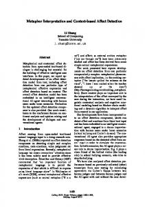
Pragmatic listener, given level-1 Interpretation

4 3 0

1

2

Probability density

5

6

7

Threshold prior Threshold posterior Height prior Height posterior

0.0

0.2

0.4

0.6

0.8

1.0

Height

Figure 1

Interpretation when tall is treated as a level-1 context-sensitive expression. The model predicts several core properties of relative adjectives: vagueness, borderline cases, and sensitivity to statistical priors.

will be shifted accordingly, while maintaining the same shape relative to the prior mean and standard deviation. Background knowledge, in the form of a statistical prior on answers to the QUD, thus interacts with lexical meaning and the pragmatic preference for informativity to yield a context-sensitive probabilistic meaning. Second, the inferred meaning of “tall” is essentially “significantly greater than average height”, an intuition which has been expressed in the literature in various forms (e.g., Fara 2000; Kennedy 2007). Crucially, though, the resulting interpretation remains vague: the interpreter maintains uncertainty about the contextual interpretation of tall, but this uncertainty does not prevent her from inferring that it does have a meaning, or from learning something about Al’s height from the utterance. Finally, the existence of borderline cases is predicted straightforwardly: if Al’s height falls around the posterior mean of θtall (height ≈ .7), he has equal probability of counting as “tall” and “not tall” in the current context, and we are thus maximally uncertain about the appropriateness of each label. The model of pragmatic interpretation sketched here, with threshold values and other semantic variables passed up to the pragmatic listener, interacts with our simple free-variable semantics to predict several of the key properties of relative adjectives in the positive form. In the next section we will consider the model’s predictions about interpretation with different types of priors. After that we return to a discussion of vagueness and the sorites paradox.

597

Lassiter & Goodman

4

Absolute adjectives

Absolute adjectives such as wet/dry, dangerous/safe, and full/empty differ from relative adjectives such as tall/short in a number of ways. As Rotstein & Winter (2004); Kennedy & McNally (2005); Kennedy (2007) and others have discussed, their meanings seem to admit of less uncertainty than those of relative adjectives, have little or no borderline region, and appear to be less susceptible to the sorites paradox (see Kennedy 2007 for detailed discussion). In this section we show that our model is able to account for these phenomena as well, given certain assumptions about the form of priors appropriate to different properties. A puzzle which has caught the attention of many semanticists in recent years is the correlation between the relative/absolute distinction and a certain topological property of scales: the presence or absence of inherent endpoints. Kennedy (2007) points out that absolute adjectives can occur only on scales with endpoints, and that there is a strong correlation between lack of endpoints and relative interpretation. He observes that theories of the positive form developed with only relative adjectives like tall in mind fail to predict the second observation: since there is no barrier to defining a context-dependent threshold on a bounded scale, relative meanings should be generally available. A major desideratum for a theory of adjectives, then, is to explain the correlation between boundedness and absolute interpretations. Kennedy (2007) claims that the meaning of a positive-form adjective associated with a bounded scale is always anchored to one of the endpoints. The proposed theoretical explanation invokes a principle of Interpretive Economy (IE): “Maximize the contribution of the conventional meanings of the elements of a sentence to the computation of its truth conditions”. Kennedy uses this principle to account for the correlation between boundedness and absolute interpretation, and argues in addition that absolute adjectives do not admit of vagueness, context-sensitivity, or borderline cases at all. Lingering uncertainty about the applicability of absolute adjectives in some cases is accounted for by invoking a qualitatively different kind of uncertainty — imprecision (Lasersohn 1999). This analysis is insightful, but some conceptual and empirical problems remain. First, the theoretical status of IE is unclear: as Potts (2008: 5) puts it, it is “an optimization principle left unsupported by a theory of optimization”. Second, there are several counter-examples to the generalization that relative and/or vague adjectives never fall on bounded scales. Kennedy (2007) himself (fn. 30) points out that bald, “the philosophers’ favorite vague adjective”, lives on a bounded scale and behaves like an absolute adjective with respect to degree modification even though it is vague. Expensive and cheap also appear to be counter-examples, since they are clearly relative adjectives, and their scale is intuitively lower-bounded by the point of zero cost. Kennedy suggests accounting for this pair by stipulating lexically

598

Context, scale structure, statistics, and adjective interpretation

that their linguistic scale excludes the zero point, even though the conceptual cost scale includes it. However, Lassiter (2010) argues that this move is ad hoc, and that additional exceptions exist including heavy/lightweight, (un)likely, and (im)probable. It is not clear whether lexical exclusion of counter-examples is a theoretically acceptable tactic; however, it does seem clear that much of the attraction of the IE-based theory is lost if problematic cases must be explained away by positing counter-intuitive scale structures. A further issue is the relative use of full noted by Kennedy & McNally (2005); McNally (2011), such as the convention of referring to a wine glass as “full” when its content is around the half-way mark. Presumably we should adopt only as a last resort a theory on which that the linguistic scale associated with full is bounded or unbounded, depending on whether the adjective describes a container whose contents are derived from grapes or grain. It would be better to have a theory which explained why the convention of filling wine glasses to a lower proportion of the total volume than beer glasses should influence the interpretation of the positive form of the adjective full. Our approach, in contrast, is embedded in a general pragmatic theory and is able to explain the correlation in question while also allowing for deviations under certain conditions. We suggest that the relevant mathematical property is a measure-theoretic one which generalizes the topological property of boundedness: prototypical relative interpretations arise with priors with a relatively mild rate of change and little or no mass on the endpoints, while prototypical absolute interpretations arise with priors in which a significant portion of the prior mass falls close to an upper or lower bound. The following figures illustrate. We suggest that the Beta(1,9) prior in figure 2, which is skewed toward the zero point, has appropriate qualitative features for min/max adjective pairs such as dangerous/safe. The probability that something counts as dangerous increases rapidly as its degree of danger deviates from the zero point, and the probability that it counts as safe decreases similarly (though slightly faster). Figure 3, with a uniform prior, likewise captures key features of the interpretation of max/max pairs such as full/empty: both indicate proximity to (though not necessarily identity with) an endpoint. (Note that a uniform prior may not be appropriate here: a prior with most of the mass at one or the other endpoint might be more realistic. If so, the change would merely strengthen the model’s preference for extreme interpretations of full and empty.) In both cases, the range over which the adjective’s applicability is uncertain is much smaller than it is in the case of tall. Our model derives the observation that absolute adjectives are less vague than relative adjectives in the positive form, but does so without appealing to distinct theoretical mechanisms. The distinction is not in the relevant kind of uncertainty, but in the amount and distribution of uncertainty.

599

Lassiter & Goodman

"Safe", lower-bounded prior 10

10

"Dangerous", lower-bounded prior

8 6 2 0 0.0

0.2

0.4

0.6

0.8

1.0

0.0

Degree of danger

Figure 2

Threshold prior Threshold posterior Danger prior Danger posterior

4

Probability density

6 4 0

2

Probability density

8

Threshold prior Threshold posterior Danger prior Danger posterior

0.2

0.4

0.6

0.8

1.0

Degree of danger

Qualitatively different statistical priors give rise to different, sometimes absolute-like interpretations. With a prior favoring low values, a nonzero but still small degree is required for the positive adjective, and a near-minimal degree for the negative adjective (generated from the positive adjective by replacing “>” with “ θtall ∣u = “xm is tall”) = P([µtall (xm ) − θtall ] ≥ ε∣u = “xm is tall”)

We can use the samples from PL1 (A,θtall ∣u) drawn in our “tall”-simulation to approximate this probability for various values of ε. As long as ε is small, the inductive premise has quite high probability: for example, with ε = .01, P(xm−1 is tall∣u = “xm is tall”) ≈ .9. We thus predict that the inductive premise of the “tall”-sorites is intuitively compelling if the step size ε in our sorites sequence is large enough. However, the argument’s conclusion is not a valid inference. According to the simulation, if André is very tall (say, .9) and Danny is very short (.1), the first and second premises of (19) will have high probability, but the third has very low probability. This is consistent because repeated use of a premise with non-maximal probability does not preserve high probability of a conclusion (see Kyburg 1961; Adams 1975, 1998). Semantically, then, the shift to a Bayesian perspective seems to dissolve the paradox as long as the gloss in (19) is reasonable.9 This model may also help to account for Kennedy’s (2007) observation that the sorites is less compelling with absolute adjectives. (21)

a. An activity with no danger attached to it is safe. b. A activity which is slightly more dangerous than a safe activity is also safe. c. ∴ A hugely dangerous activity is safe.

Unlike (18b), the inductive premise (21b) does not seem to be intuitively compelling. With ε = .1 and the prior used in the simulation above, the probability that a “safe” object will fall with ε of the threshold is less than .7. This is much lower than in the case of “tall”, and so we do not expect that the inductive premise will be as compelling with “safe” as it is with “tall”. 6

Conclusion

Our model of adjective interpretation is an application of a general pragmatic model which emphasizes the continuity of language understanding and uncertain reasoning 9 This account is of necessity very brief, and does not address other variants of the paradox. See Edgington 1997; Lassiter 2011a; Égré 2011 for additional discussion of the probabilistic account of the sorites with relative adjectives. Note in particular that the case is even clearer with the negative existential variant of the inductive premise, whose probabilistic rendition asserts that there is no sudden transition from high to low probability (Lassiter 2011a).

604

Context, scale structure, statistics, and adjective interpretation

and decision-making in other areas of cognition. Adopting a simple free-variable semantics for adjectives, we have applied tools from Bayesian modeling to predict context-sensitive meanings. The model we proposed derives novel quantitative and qualitative predictions about adjective interpretation, suggesting a new explanation of the vagueness and context-sensitivity of relative adjectives, the existence of borderline cases, and the absolute-relative distinction and its interaction with the sorites paradox. Some of the choices that we have made in setting up the model are overly simplified, such as the assumption that speakers care only about informativity and cost. The interpretive effects of rich speaker goals remain to be explored, as does varying the QUD and numerous other possible enrichments and modifications of the model. Likewise, our account of the relative/absolute distinction relies to a considerable extent on intuitions about reasonable priors to assume for specific properties. It will be necessary to refine the choice of priors using experimental and corpus investigation, and also to validate the assumed posterior distributions experimentally. Other natural extensions of the model include inferring the QUD (Kao, Wu, Bergen & Goodman 2014) and choosing the relevant scale for adjectives for which there are several options (Kennedy 1997; Sassoon 2013). We hope that this work will be seen as a demonstration of the potential for fruitful interaction between formal semantics/pragmatics and cognitive science (see also Goodman & Lassiter 2014). Bayesian modeling makes it possible to combine logical and probabilistic reasoning seamlessly, opening up new opportunities for exploring how listeners use context and background knowledge to construct rich context-sensitive interpretations in the presence of uncertainty. References Adams, Ernest W. 1975. The Logic of Conditionals: An Application of Probability to Deductive Logic. Springer. Adams, Ernest W. 1998. A Primer of Probability Logic. Center for the Study of Language and Information. Bale, Alan C. 2011. Scales and comparison classes. Natural Language Semantics 19. 169–190. Barker, Chris. 2002. The dynamics of vagueness. Linguistics and Philosophy 25(1). 1–36. Bartsch, Renate & Theo Vennemann. 1973. Semantic Structures: A Study In the Relation Between Semantics and Syntax. Athenäum. Benz, Anton, Gerhard Jäger & Robert van Rooij. 2005. Game Theory and Pragmatics. Palgrave Macmillan. Bergen, Leon, Noah D. Goodman & Roger Levy. 2012. That’s what she (could

605

Lassiter & Goodman

have) said: How alternative utterances affect language use. In David Peebles Naomi Miyake & Richard P. Cooper (eds.), Thirty-Fourth Annual Meeting of the Cognitive Science Society, 120–125. Cognitive Science Society. Burnett, Heather. 2014. A Delineation Solution to the Puzzles of Absolute Adjectives. Linguistics and Philosophy 37(1). 1–39. Clark, H.H. 1996. Using Language. Cambridge University Press. Edgington, Dorothy. 1995. On conditionals. Mind 104(414). 235. doi:10.1093/mind/104.414.235. Edgington, Dorothy. 1997. Vagueness by degrees. In Rosanna Keefe & Peter Smith (eds.), Vagueness: A Reader, 294–316. MIT Press. Égré, Paul. 2011. Perceptual ambiguity and the sorites. In Rick Nouwen, Robert van Rooij, Uli Sauerland & Hans-Christian Schmitz (eds.), Vagueness in Communication, 64–90. Springer. Fara, Delia Graff. 2000. Shifting sands: An interest-relative theory of vagueness. Philosophical Topics 20. 45–81. Fine, Kit. 1975. Vagueness, truth and logic. Synthese 30(3). 265–300. Fox, Danny & Roni Katzir. 2011. On the characterization of alternatives. Natural Language Semantics 19(1). 87–107. Frank, M.C. & N.D. Goodman. 2012. Predicting pragmatic reasoning in language games. Science 336(6084). 998–998. Franke, M. 2009. Signal to act: Game theory in pragmatics: University of Amsterdam dissertation. Franke, Michael. 2012a. On Scales, Salience and Referential Language Use. In Maria Aloni, Floris Roelofsen & Katrin Schulz (eds.), Amsterdam Colloquium 2011, Springer. Franke, Michael. 2012b. Scales, Salience and Referential Safety: The Benefit of Communicating the Extreme. In Thomas C. Scott-Phillips, Mónica Tamariz, Erica A. Cartmill & James R Hurford (eds.), The Evolution of Language: Proceedings of the 9th International Conference (EvoLang 9), 118–125. Frazee, Joey & David Beaver. 2010. Vagueness is rational under uncertainty. In Maria Aloni, Harald Bastiaanse, Tikitu de Jager & Katrin Schulz (eds.), Logic, Language and Meaning: 17th Amsterdam Colloquium, Amsterdam, The Netherlands, December 16-18, 2009, Revised Selected Papers, 153–162. Springer. Ginzburg, Jonathan. 1995a. Resolving questions, I. Linguistics and Philosophy 18(5). 459–527. Ginzburg, Jonathan. 1995b. Resolving questions, II. Linguistics and Philosophy 18(6). 567–609. Golland, Dave, Percy Liang & Dan Klein. 2010. A game-theoretic approach to generating spatial descriptions. In Empirical Methods in Natural Language Processing (EMNLP), 410–419.

606

Context, scale structure, statistics, and adjective interpretation

Goodman, N.D. & A. Stuhlmüller. 2012. Knowledge and implicature: Modeling language understanding as social cognition. Topics in Cognitive Science 5(1). 173–184. Goodman, Noah D. & Daniel Lassiter. 2014. Probabilistic semantics and pragmatics: Uncertainty in language and thought. In Shalom Lappin & Chris Fox (eds.), Handbook of Contemporary Semantic Theory, Wiley-Blackwell 2nd edn. Grice, H. Paul. 1957. Meaning. The Philosophical Review 66(3). 377–388. Grice, H. Paul. 1989. Studies in the Way of Words. Harvard University Press. Griffiths, Thomas L., Charles Kemp & Joshua B. Tenenbaum. 2008. Bayesian models of cognition. In Ron Sun (ed.), Cambridge Handbook of Computational Psychology, 59–100. Cambridge University Press. Jacobson, Pauline. 1999. Towards a variable-free semantics. Linguistics and Philosophy 22(2). 117–185. Jäger, Gerhard. 2007. Game dynamics connects semantics and pragmatics. Game theory and linguistic meaning 18. 103. Kamp, Hans. 1975. Two theories about adjectives. In E. Keenan (ed.), Formal Semantics of Natural Language, 123–155. Cambridge University Press. Kao, Justine T., Jean Y. Wu, Leon Bergen & Noah D. Goodman. 2014. Nonliteral language understanding for number words. Manuscript, Stanford University and MIT. Katzir, Roni. 2007. Structurally-defined alternatives. Linguistics and Philosophy 30(6). 669–690. Kehler, Andrew & Hannah Rohde. 2012. Grammatical and information-structural influences on pronoun production. To appear in Language and Cognitive Processes. Kehler, Andrew & Hannah Rohde. 2013. A probabilistic reconciliation of coherencedriven and centering-driven theories of pronoun interpretation. Theoretical Linguistics 1–37. Kennedy, Chris. 1997. Projecting the adjective: The syntax and semantics of gradability and comparison: U.C., Santa Cruz dissertation. Kennedy, Chris. 2007. Vagueness and grammar: The semantics of relative and absolute gradable adjectives. Linguistics and Philosophy 30(1). 1–45. Kennedy, Chris & Louise McNally. 2005. Scale structure, degree modification, and the semantics of gradable predicates. Language 81(2). 345–381. Klein, Ewan. 1980. A semantics for positive and comparative adjectives. Linguistics and Philosophy 4(1). 1–45. Kyburg, Henry. 1961. Probability and the Logic of Rational Belief. Wesleyan University Press. Lasersohn, Peter. 1999. Pragmatic halos. Language 522–551. Lassiter, Daniel. 2010. Gradable epistemic modals, probability, and scale structure.

607

Lassiter & Goodman

In Nan Li & David Lutz (eds.), Semantics & Linguistic Theory (SALT) 20, 197–215. CLC Publications. Lassiter, Daniel. 2011a. Measurement and Modality: The Scalar Basis of Modal Semantics: New York University dissertation. Lassiter, Daniel. 2011b. Vagueness as probabilistic linguistic knowledge. In R. Nouwen, R. van Rooij, U. Sauerland & H.-C. Schmitz (eds.), Vagueness in Communication, 127–150. Springer. Lassiter, Daniel. 2012. Presuppositions, provisos, and probability. Semantics & Pragmatics 1–37. Lewis, David. 1969. Convention: A Philosophical Study. Harvard University Press. Luce, R. Duncan. 1959. Individual Choice Behavior: A Theoretical Analysis. John Wiley. MacKay, David J.C. 2003. Information Theory, Inference, and Learning Algorithms. Cambridge University Press. McNally, Louise. 2011. The relative role of property type and scale structure in explaining the behavior of gradable adjectives. In Rick Nouwen, Robert van Rooij, Uli Sauerland & Hans-Christian Schmitz (eds.), Vagueness in Communication, 151–168. Springer. Neal, Radford M. 1993. Probabilistic inference using markov chain monte carlo methods. Technical Report CRG-TR-93-1, Department of Computer Science, University of Toronto. Pearl, Judea. 2000. Causality: Models, reasoning and inference. Cambridge University Press. Potts, Christopher. 2008. Interpretive Economy, Schelling points, and evolutionary stability. Ms., University of Massachusetts at Amherst. Roberts, Craige. 1996. Information structure in discourse: Towards an integrated formal theory of pragmatics. Working Papers in Linguistics-Ohio State University Department of Linguistics 91–136. Rotstein, Carmen & Yoad Winter. 2004. Total adjectives vs. partial adjectives: Scale structure and higher-order modifiers. Natural Language Semantics 12(3). 259–288. Sapir, Edward. 1944. Grading: A study in semantics. Philosophy of Science 11(2). 93–116. Sassoon, Galit W. 2013. A typology of multidimensional adjectives. Journal of Semantics 30(3). 335–380. Schmidt, Lauren, Noah D. Goodman, David Barner & Joshua Tenenbaum. 2009. How tall is Tall? Compositionality, statistics, and gradable adjectives. In Niels Taatgen & Hedderik van Rijn (eds.), 31st Annual Conference of the Cognitive Science Society, 3151–3156. Shannon, Claude E. 1948. A mathematical theory of communication. Bell System

608

Context, scale structure, statistics, and adjective interpretation

Technical Journal 27. 379–423. Smith, Nathaniel J, Noah Goodman & Michael Frank. 2013. Learning and using language via recursive pragmatic reasoning about other agents. In Christopher J.C. Burges, Léon Bottou, Max Welling, Zoubin Ghahramani & Kilian Q. Weinberger (eds.), Advances in Neural Information Processing Systems 26, 3039–3047. Curran Associates, Inc. Solt, Stephanie. 2011. Notes on the comparison class. In Rick Nouwen, Robert van Rooij, Uli Sauerland & Hans-Christian Schmitz (eds.), Vagueness in Communication, 127–150. Springer. Stalnaker, Robert. 1978. Assertion. In Peter Cole (ed.), Syntax and Semantics 9: Pragmatics, Academic Press. von Stechow, Arnim. 1984. Comparing semantic theories of comparison. Journal of Semantics 3(1). 1–77. Sutton, Peter. 2013. Vagueness, Communication and Semantic Information: King’s College London dissertation. Sutton, Richard S. & Andrew G. Barto. 1998. Reinforcement Learning: An Introduction. MIT Press. Tenenbaum, Joshua B., Charles Kemp, Tom L. Griffiths & Noah D. Goodman. 2011. How to grow a mind: Statistics, structure, and abstraction. Science 331(6022). 1279. http://www.cogsci.northwestern.edu/speakers/2011-2012/ tenenbaumEtAl_2011-HowToGrowAMind.pdf. Unger, Peter. 1971. A defense of skepticism. The Philosophical Review 80(2). 198–219. Vogel, Adam, Max Bodoia, Christopher Potts & Dan Jurafsky. 2013a. Emergence of Gricean maxims from multi-agent decision theory. In Human Language Technologies: The 2013 Annual Conference of the North American Chapter of the Association for Computational Linguistics, 1072–1081. Stroudsburg, PA: Association for Computational Linguistics. Vogel, Adam, Christopher Potts & Dan Jurafsky. 2013b. Implicatures and nested beliefs in approximate Decentralized-POMDPs. In Proceedings of the 2013 Annual Conference of the Association for Computational Linguistics, 74–80. Stroudsburg, PA: Association for Computational Linguistics. Williamson, Timothy. 1994. Vagueness. Routledge. Xu, Fei & Joshua B. Tenenbaum. 2007. Word learning as Bayesian inference. Psychological Review 114(2). 245.

609

Lassiter & Goodman

Noah D. Goodman Stanford Psychology Building 420, Jordan Hall 450 Serra Mall Stanford, CA 94305 [email protected]

Daniel Lassiter Stanford Linguistics Building 460, Margaret Jacks Hall 450 Serra Mall Stanford, CA 94305 [email protected]

610