buying in a selling market context than in a buying market. In order for ...... J. (1995). The New Market Wizards: Conversations with America's Top Traders, Wiley.
GLOBAL JOURNAL OF BUSINESS RESEARCH ♦ VOLUME 5 ♦ NUMBER 5 ♦ 2011
CONTEXT SENSITIVITY WITH NEURAL NETWORKS IN FINANCIAL DECISION PROCESSES Charles Wong, Boston University Massimiliano Versace, Boston University ABSTRACT Context modifies the influence of any trading indicator. Ceteris paribus, a buyer would be more cautious buying in a selling market context than in a buying market. In order for automated, adaptive systems like neural networks to better emulate and assist human decision-making, they need to be context sensitive. Most prior research applying neural networks to trading decision support systems neglected to extract contextual cues, rendering the systems blind to market conditions. This paper explores the theoretical development and quantitative evaluation of context sensitivity in a novel fast learning neural network architecture, Echo ARTMAP. The simulated risk and cost adjusted trading results compare very favorably on a 10-year, random stock study against the market random walk, regression, auto-regression, and multiple neural network models typically used in prior studies. By combining human trader techniques with biologically inspired neural network models, Echo ARTMAP may represent a new tool with which to assist in financial decision-making and to explore life-like context sensitivity. JEL: G11, G17 KEYWORDS: Recurrent neural networks, context sensitivity, financial forecasting, investment decisions INTRODUCTION
S
tock prices refer to the latest mutually decided transaction price and time between a voluntary buyer and seller. If the stock prices over time are increasing, they indicate that the buying interest exceeds the selling interest. This signals a bullish or optimistic market context favorable to investment, all else equal. A successful trader (Schwager, 1994) often considers the underlying market sentiment when making decisions. This sensitivity to context in decision-making is one of the hallmarks of human intelligence (Akman, 2002). Human subjects often treat similar tasks differently under different contexts (e.g. Carraher, Carraher, & Schliemann, 1985; Bjorklund & Rosenblum, 2002). Working memory allows features to be tracked over time to extract a context (Kane & Engle, 2002; Baddeley & Logie, 1999). Context sensitivity theoretically enables the decision-maker to disambiguate different feature inputs that may be identical at single points in time (Kane & Engle, 2002). To better model human decision-making with context sensitivity, an automatic decision system must be context sensitive (see Figure 1, left). Tracking the price over time to determine whether the market is uptrending (bullish) or downtrending (bearish) intuitively provides contextual cues (Schwager, 1994). This paper introduces a context sensitive neural network decision system, Echo ARTMAP.
27 Electronic copy available at: http://ssrn.com/abstract=1874850
C Wong & M. Versace | GJBR ♦ Vol. 5 ♦ No. 5 ♦ 2011
Figure 1: Extracting Contextual Patterns from Historical Prices Price (x)
Price (x)
12000
12000
9000
9000
BUY
6000
SELL
BUY
SELL
6000
June, 2008 June, 2009 June, 2008 June, 2009 Figure 1: One-year daily prices for the Dow Jones Industrial Average. (left) Identical point inputs (the horizontal line indicates same price) lead to different classes. The boxes show different contexts that can disambiguate the two inputs. (right) Identical short duration inputs (small boxes) lead to different classes. The longer duration input (large boxes) can disambiguate the two inputs.
The remaining sections of this paper divide as follows: Section II reviews the recent literature applying neural models to financial time series. Section III provides a brief review of the default ARTMAP neural network kernel mechanism as a base for later extension; Section IV demonstrates how to theoretically adapt the ARTMAP to context sensitivity; Section V outlines the data and methodology; Section VI provides the results and discussion; and Section VII contains concluding remarks. LITERATURE REVIEW Neural networks are biologically inspired, automated, and adaptive analysis models that can better accommodate non-linear, non-random, and non-stationary financial time series than alternatives (e.g. Lo, 2001; Lo & Repin, 2002; Lo, 2007; Gaganis, Pasiouras, & Doumpos, 2007; Yu, Wang, & Lai, 2008). Much research in the past decade applies them to financial time series with typically strong and compelling empirical results. Our survey of 25 studies published in the past decade (Wong & Versace, 2011a) divides the network models into four categories with breakdowns: (1) slow learning context blind, 56%; (2) fast learning context blind, 28%; (3) slow learning context sensitive, 16%; and (4) fast learning context sensitive, 0%. Saad, et al. (1998), compare multiple neural models on financial forecasting accuracy. Data included the daily prices for 10 different stocks over one year representing high volatility, consumer, and cyclical industries. Models included a fast learning radial basis function, a slow learning backpropagation network, and a slow context sensitive recurrent backpropagation model. Results showed that all three networks provided similar performance. Versace, et al. (2004), apply genetic algorithms to determine the network, structure, and input features for financial forecasting. Data included 300 daily prices from the Dow Jones Industrial Average. Features included a series of technical indicators. Models included both fast learning and slow context sensitive networks. Results showed that using a genetic algorithm to choose and design the network and features could generate significant accuracy in trading decisions. Sun, et al. (2005), use a fast learning neural model for time series. Data included two years of daily S&P 500 and Shanghai Stock Exchange indices. Their model updates the fast learning radial basis function with a novel Fisher’s optimal partition algorithm for determining basis function centers and sizes with
28 Electronic copy available at: http://ssrn.com/abstract=1874850
GLOBAL JOURNAL OF BUSINESS RESEARCH ♦ VOLUME 5 ♦ NUMBER 5 ♦ 2011
dynamic adjustment. improvements.
Results show that the updated fast learning model provides significant
Zhang, et al. (2005), explore slow learning backpropagation networks for financial time series analysis. Data included seven years of daily Shanghai Composite Index data. Enhancements to the slow learning model apply normalization and kernel smoothing to reduce noise. Results show that the slow learning models consistently outperformed the buy-and-hold strategy. Chen & Shih, (2006), apply neural network models to six Asian stock markets, including Nikkei, Hang Seng, Kospi, All Ordinaries, Straits Times, and Taiwan Weighted indices. Features included five technical analysis indicators. Models included fast learning support vector machines and the slow learning backpropagation. Results show that the neural models outperformed autoregression models, especially with respect to risk. The fast learning models also appear to outperform the slow learning models. Ko & Lin, (2008), apply a modified slow learning backpropagation model to a portfolio optimization problem on 21 companies from the Taiwan Stock Exchange for five years. Results show that their resource allocation neural network outperformed the buy-and-hold considerably, averaging 15% to 5% yearly gains. Freitas, et al. (2009), apply an enhanced slow learning context sensitive model to weekly closing prices for 52 Brazilian stocks for 8 years. Their model uses recurrence to increase emphasis towards more recent data. Results show that their model produced results in excess of the mean-variance model and the market index with similar levels of risk. In all remaining cases, the neural networks appear outperform random walk or buying-and-holding approaches to the financial time series. The results appear robust regardless of network learning rule or context sensitivity. The bias towards slow learning networks probably reflects their earlier availability (Rumelhart, Hinton, & Williams, 1986). Of the studies employing context sensitive models, all relied on slow learning rules incorporated in Jordan and Elman networks (e.g. Versace et al, 2004; Yu, Wang, & Lai, 2008; Freitas, Souza, & Almeida, 2009; Jordan, 1986; Elman, 1990). Studies directly comparing fast learning, slow learning, and slow learning context sensitive networks have found no significant differences in empirical results (e.g. Saad et al, 1998). This paper explores the disagreement between the intuition supporting the importance of context sensitivity and the empirical results showing no differential benefit relative to existing neural network models. The bulk of the studies indicate existing models tend not to incorporate fast learning with context in finance. Therefore, this paper introduces a novel context sensitive fast learning network, Echo ARTMAP, for transparent analysis (Moody & Darken, 1989; Carpenter, Grossberg, & Reynolds, 1991; Parsons & Carpenter, 2003). The base fast learning component model is ARTMAP (Amis & Carpenter, 2007) from the Adaptive Resonance Theory class of models. While ARTMAP is not a perfect blend of all existing fast learning characteristics (e.g. it differs in learning vs. Radial Basis Function networks), it can be regarded as a general purpose, default network that automatically adapts and scales its topology to a generic dataset (e.g. Carpenter, 2003). For this paper, benchmarks include random walk, regression, auto-regression, a slow learning backpropagation (Rumelhart, Hinton, & Williams, 1986), a fast learning ARTMAP (Amis & Carpenter, 2007), and a slow learning context sensitive model (Jordan, 1986). Kernel Review for a Typical Fast Learning Model Slow learning networks possess hidden layers that have opaque representations relating inputs to outputs. In contrast, fast learning allows immediate and transparent convergence for independent storage layer 29
C Wong & M. Versace | GJBR ♦ Vol. 5 ♦ No. 5 ♦ 2011
nodes. ARTMAP is a type of fast learning network that was inspired by biological constraints and can be adapted to a variety of uses. Extensive literature shows its capabilities and interprets its mathematical bases (e.g. Amis & Carpenter, 2007; Parsons & Carpenter, 2003). Figure 2 (left) shows the default ARTMAP flow diagram. Figure 2: A Typical General Purpose Fast Learning Neural Model, ARTMAP Input
X
Storage
Output Normalize
W1
Complement code
Fuzzy min
Sum
(0.5,0.3)
(0.8)
1 Wj
W2
WJ
BUY
SELL
0.7
X
0.5
(0.7,0.3) (0.5,0.5)
0 ARTMAP Kernel:
| X ∧W j |
Figure 2: (left) A default ARTMAP network diagram showing the three-layer architecture. For a particular input pattern,
X
the ARTMAP
kernel finds the most similar stored pattern, W j which maps to a specific output node. Boxes, or nodes, represent patterns (responses in the output layer) and circles represent individual components of the pattern. (right) This is an example of the ARTMAP kernel calculating the similarity between an input pattern and a single stored pattern. See the text for details.
There are three layers in the default ARTMAP network. The input layer receives input patterns, each represented by a vector with one or more components, X . Given this vector, the network finds the most similar vector W j from the storage layer, where j = {1...J} and J is the number of storage nodes. The output layer node associated with the most similar storage node dictates the network response. The ARTMAP kernel, which is a function that determines the similarity between vectors (Bishop, 2006), models pattern recognition as per equation (1):
T j =| X ∧ W j | ,
(1)
where T j is the similarity score for storage node j. The kernel procedure has four steps: normalize all vector component values to between 0 and 1; complement code both vectors such that X = ( x1 ,1 − x1 ) ; apply the fuzzy min operator (^) on the vectors; and sum (||). For example, given a normalized input value of 0.5 and a particular normalized storage node of 0.7, the complement codes would be (0.5, 0.5) and (0.7, 0.3). The fuzzy min would be the lesser of each component, or (0.5, 0.3) and their sum would be 0.8, which as a normalized value can also be read as 80% similar. The default ARTMAP learning rules that update and add storage layer nodes with their associated output nodes are not modified and are not treated here. For references on previously published ARTMAP models, please see http://techlab.bu.edu. The following section provides the theoretical modifications to this kernel.
30
GLOBAL JOURNAL OF BUSINESS RESEARCH ♦ VOLUME 5 ♦ NUMBER 5 ♦ 2011
Extracting Context The approach taken here explores fast learning network rules with context sensitivity. Figure 3 shows how a fast learning ARTMAP model can be modified to process time patterns in the data with three steps via input delays, decays, and output-to-input recurrence to create the novel Echo ARTMAP model. Figure 3: Echo ARTMAP Extends the General Purpose Neural Model for Context Input
Storage
X
Output
W1 Feedback w/Input
W2
Translate Feedback
Expanded Input
BUY= BUY SELL=
WJ
SELL Echo ARTMAP ' Kernel T j =| A . * X + (1 − A) |
Figure 3: (left) The full Echo ARTMAP architecture with time delay, decay, and recurrence. See text for the breakdown of the three steps. (right) Excerpted from figure 1, the feedback provides additional input information from past storage values. Translating the feedback back into its component pattern allows more information to be input into the network. This example assumes the patterns in Figure 1, left, have already been stored, for instance allowing the feedback Buy value to be translated into an uptrend. This process can be repeated infinitely, allowing greatly expanded inputs.
Implementing input time delays allows an ARTMAP network to model one aspect of working memory. Figure 3 (left) shows the ARTMAP network from figure 2 with multiple components in each node, the right two being the same feature at different points in time. Similarity proceeds from equation (1), but depends on multiple points in time. Figure 4 (a and b) compares the influence of a given input over time when introducing input time delay. With no delay, the network at time t can only consider inputs from time t. Figure 4: Graphical Representation of Past Influence on Decision with Context Sensitivity (a)
(b)
(c)
(d)
Influence
t-3
t-2 Time
t-1
t
t-3
t-2 Time
t-1
t
t-3
t-2 Time
t-1 t
t-3
t-2
t-1
t
Time
Figure 4: The influence of past inputs at time t. (a) At time t, a model with no time delay only considers the current input from t. (b) A model with a delay of 2 considers both the input from t and the past two inputs equally. (c) A model with delay of 2 with decay considers the input from t and the past two inputs, but with more emphasis on more current inputs. (d) A model with delay of 2 with decay and output-to-input recurrence theoretically considers all prior inputs albeit with very little emphasis on distant inputs in time.
Implementing time decay allows an ARTMAP network to model a more complex, non-stationary working memory. In a non-stationary data set, proximal points in time should have more influence than distal points in time (Hamilton, 1994). The underlying state or context is shifting over time, such that 31
C Wong & M. Versace | GJBR ♦ Vol. 5 ♦ No. 5 ♦ 2011
feature values within the current state are more relevant. Equation (2) shows how to scale the contextual importance:
T j =| A . * X '+(1 − A) | ,
(2)
where X ' = X ∧ W j , or the component-wise collection after the first three steps in equation (1), A = (a1 , a 2 ,...a M ) , 0