Contextual Building Selection Based on a Genetic Algorithm in ... - MDPI

International Journal of

Geo-Information Article

Contextual Building Selection Based on a Genetic Algorithm in Map Generalization Lin Wang 1 1 2 3 4

*

ID

, Qingsheng Guo 1,2, *

ID

, Yuangang Liu 3 , Yageng Sun 4 and Zhiwei Wei 1

School of Resource and Environmental Science, Wuhan University, Wuhan 430079, China; [email protected] (L.W.); [email protected] (Z.W.) State Key Laboratory of Information Engineering in Surveying, Mapping and Remote Sensing, Wuhan University, Wuhan 430079, China School of Geoscience, Yangtze University, Wuhan 430010, China; [email protected] Wuhan Geomatics Institute, Wuhan 430022, China; [email protected] Correspondence: [email protected]; Tel.: +86-138-7144-1265

Received: 6 July 2017; Accepted: 28 August 2017; Published: 30 August 2017

Abstract: In map generalization, scale reduction and feature symbolization inevitably generate problems of overlapping objects or map congestion. To solve the legibility problem with respect to the generalization of dispersed rural buildings, selection of buildings is necessary and can be transformed into an optimization problem. In this paper, an improved genetic algorithm for building selection is designed to be able to incorporate cartographic constraints related to the building selection problem. Part of the local constraints for building selection is used to constrain the encoding and genetic operation. To satisfy other local constraints, a preparation phase is necessary before building selection, which includes building enlargement, local displacement, conflict detection, and attribute enrichment. The contextual constraints are used to ascertain a fitness function. The experimental results indicate that the algorithm proposed in this article can obtain good results for building selection whilst preserving the spatial distribution characteristics of buildings. Keywords: building generalization; selection operator; genetic algorithm; contextual information

1. Introduction Map generalization aims to represent geographic information in an abstract way when deriving small-scale maps from larger-scale ones. It has long been a core issue in automated map production and multi-scale spatial representation [1–3]. Among the various data themes, the building features have attracted much research attention in the field of map generalization because of their man-made shape and complex spatial distribution. Scale reduction and feature symbolization in building generalization inevitably generate spatial conflicts of proximity and overlap, which reduce the readability of maps. To solve such conflicts, cartographers have conducted a great deal of research [4–12]. In these approaches, displacement has been the major generalization operator [4–9]. However, displacement itself does not guarantee that all conflicts are resolved, especially when the map space available is insufficient. As one of the contextual operators, building selection, which can also be referred to as building elimination, is aimed at reducing the number of buildings under specific cartographic rules. When the density is too high to displace buildings while not high enough to aggregate them, selection should be used to eliminate the conflicts. At present, most selection algorithms have been developed for point set [13–19]. In terms of building selection, existing studies have focused either on local elimination [20,21] or on elimination of buildings with a regular distribution such as linear-structured buildings [11,22–24]. Therefore, it is necessary to find effective building selection approaches for irregularly distributed buildings, especially when their overall density is high. ISPRS Int. J. Geo-Inf. 2017, 6, 271; doi:10.3390/ijgi6090271

www.mdpi.com/journal/ijgi

ISPRS Int. J. Geo-Inf. 2017, 6, 271

2 of 23

Instead of the generalization of urban buildings, which has already been studied [25,26], the focus here is on the generalization of rural buildings. The main objective is to transform groups of buildings into a readable form at the target scales by extracting a new representative set of buildings. The major challenge facing the selection problem is that a set of cartographic constraints should be satisfied. For example, the result should contain as few conflicts as possible, preferably none; the spatial relationships and patterns of the original building set should be preserved as much as possible after the selection process. This implies that selection can be considered as an optimization problem, where different goals have to be satisfied simultaneously. The genetic algorithm (GA) is a well-known optimization approach. The algorithm was first proposed by Holland [27] and then developed by Goldberg [28] in the field of artificial intelligence. Through simulation of biological evolutionary strategy, the algorithm is able to find the optimal or sub-optimal solution for a difficult problem from a host of feasible solutions. It has proven to be effective in building cluster displacement [29–31] and in other generalization problems such as map labeling [32] and line simplification [33]. Compared to other optimization algorithms (such as the steepest descent method and the simulated annealing algorithm), the GA has better performance under many constraints. The GA is therefore proven to be suitable for solving the building selection problem in this paper. To make the generalization solutions more attractive to cartographers, the GA has been improved to satisfy a set of cartographic constraints. First, the concept of conflicting block is introduced in the encoding and genetic operation, making all solutions free of conflicts. Then, important buildings and identified alignments are preserved in the form of fixing the corresponding genes. Finally, spatial distribution and density constraints are specified in a fitness function. By incorporating these constraints into the GA design, it can be ensured that no conflict exists among the retained buildings and that the spatial distribution characteristics are preserved to the greatest extent possible. The remainder of this paper is organized as follows. Section 2 reviews previous work on building generalization. Section 3 focuses on how to design the GA in three main compositions considering the related constraints that act on buildings. Section 4 describes the implementation of the method for the problem considered. To validate the algorithm, Section 5 presents experiments on two topographic datasets and discusses the experimental results. Finally, Section 6 concludes this study and suggests future works. 2. Related Work Over the past few decades, many research studies have been carried out on building generalization. Some of these studies have focused on the overall process of generalization. Examples include agent modeling techniques based on constraints and the Multi-Agent System (MAS) paradigm [21,34,35]; a method for building groupings and then generalizations utilizing Gestalt principles and urban morphology [25]; and a multi-parameter approach to building grouping and generalization based on three principles of Gestalt theories and six parameters [12]. Other studies have focused mainly on developing new algorithms for specific generalization operators. These algorithms can be roughly categorized into two types: non-contextual operators for an individual building like simplification [24,36], and contextual operators for building groups such as displacement, selection or typification [4–9,22–24]. Compared with other generalization operators, the specificity of selection implies the need to determine the number of objects retained in the target map according to the scale and the purposes. Töpfer and Pillewizer [37] proposed a law, known as the radical law, which allows making such a decision. Another challenge facing selection is to decide which buildings should be retained and which ones should be removed. This decision needs to take into consideration not only the characteristics of the building such as its shape and size, but also contextual information such as the relationships among the building and the road or other features, all of which add to the complexity of selection.


3 of 23

Bjørke [20] proposed an entropy-based method for feature elimination. In an example of area elimination, house symbols were set to be of equal size. The grade of similarity of any two neighboring symbols could be evaluated according to their proximity to each other. After mapping, the grade of similarity to transition probabilities, the local equivocation for each symbol, was computed. At each step, the symbol with the greatest equivocation was eliminated from the map. This process was terminated when a map index received its maximum value. Ruas [21] presented another iterative elimination algorithm. Unlike the entropy-based method, which can only consider one criterion in the process of elimination, this algorithm can consider numerous constraints simultaneously. These constraints were combined to define a cost function for each building. At each step, the elimination cost of the building was calculated, and the building with the highest value eliminated. These steps were repeated until the result satisfied a predefined criterion. As elimination algorithms can only delete one building in one iteration step, they are most suitable for situations where the local density of buildings is high. When the overall density of buildings is high, these algorithms become inapplicable. Building typification can be termed as selection with building relocation [38]. There is no clear distinction between selection and typification in some holistic process. Regnauld [11] presented a method for selection based on the typification principle. Buildings were grouped into homogeneous clusters, making use of graph theory and Gestalt principles, then the buildings in each group were analyzed, and the representation of new buildings according to each group’s information (e.g., size, orientation, length, width, etc.) were determined. This algorithm was mainly suitable for buildings with linear structures. Sester [24] adopted a neural network technique in generalization, and presented a typification algorithm based on self-organizing maps. In the algorithm, the original building point set served as the input space. A subset of the point set represented the map space. The number of points in the subset could be determined using Töpfer’s radical law [37]. Each point was a neuron, and these neurons were linked to form a network by constructing a Delaunay triangulation. The points and their neighborhoods were iteratively adjusted according to the stimuli until they approximated the distribution of the original dataset. The prominent advantage of this algorithm is that the density characteristic can be well maintained after typification. The disadvantage is that the algorithm does not take into account other constraints such as the minimum distance constraint. Burghardt and Cecconi [22] adopted a mesh simplification technique to develop a typification algorithm for buildings. The algorithm could be basically divided into two phases: positioning and representation. In the positioning phase, the target number and position of buildings were determined based on Töpfer’s radical law and Delaunay triangulation. The representation phase elaborated how to construct new buildings to replace the ones they represented in the determined position. Typification of buildings for any scale between two source scales (e.g., 1:25,000 and 1:200,000) can be achieved using this algorithm. One limitation is that no consideration was given to alignment. Gong and Wu [23] identified a linear pattern utilizing Gestalt visual perception, computational geometry, and graph theory, and then developed a typification algorithm for linear pattern buildings. They divided the typification process into three parts: elimination of buildings with minimum overall effect, exaggeration of the remaining buildings according to their relative location in the linear pattern and displacement of buildings along the linear pattern trajectory direction. By iteratively executing the above three parts, the maintenance of linear patterns could be guaranteed after typification. Building generalization is challenging because it needs to take into account spatial structure knowledge. Such knowledge is often implicit in datasets, and specific methods, such as cluster analysis and pattern recognition, should be used to make it explicit. For example, Jones et al. [36] used Delaunay triangulation for neighborhood analysis. Regnauld [39] extracted linear building clusters by constructing and segmenting a minimum spanning tree. Anders and Sester [40] proposed a parameter-free grouping method based on graph theory. Christophe and Ruas [38] identified straight-line building alignments and preserved the regular ones for typification. Li et al. [25] adopted


4 of 23

a neighborhood model form urban morphology for global partitioning and then applied Gestalt principles to group buildings locally. Basaraner and Selcuk [41] developed a structure recognition technique using of Voronoi diagrams and spatial analysis methods. Zhang et al. [42] developed two algorithms to recognize collinear and curvilinear alignments in buildings. The knowledge gained from all these studies provides useful information for successful generalization. 3. Cartographic Selection from a GA Perspective 3.1. GA Summary This section outlines the process of how to use a GA to solve an optimization problem. The core idea of the GA is to mimic Darwin’s idea of finding the optimal individual through selective reproduction in a given environment. When the GA is applied in generalization, a solution to the problem is represented using a chromosome. Each chromosome is composed of a number of genes and modeled by a string of values. A gene has two or more different versions called alleles. A certain number of chromosomal individuals make up a population. The evolutionary process is conducted on the basis of the population. The GA uses a fitness function to determine which individuals in the population can better solve a problem. Appropriate individuals are selected to generate a new generation by crossover and mutation. This process is iterated until a stop criterion is reached. The individual with the highest fitness value is considered as the best solution. The main components of a typical GA include: Encoding: transforming solutions of a problem into gene representations. Initialization: generating a set of chromosomes that represent optional solutions to the problem. Selection: selecting individuals from the current population as parents for reproduction, based on their fitness values. Crossover: producing children by recombining the genes of two parents. Mutation: randomly selecting genes in an individual and replacing them by their allele to ensure diversity. Termination criterion: stopping the algorithm when the algorithm converges or when the number of iterations reaches a pre-specified value. When using a GA to solve generalization problems, the following three key issues must be made clear in the algorithm design: 1. 2. 3.

Definition and expression of the solution to the problem, namely how to design the genes of an individual in the GA. Choice of appropriate genetic operators, such as selection, crossover, mutation, etc., to evolve the population of solutions. Definition of a fitness function to evaluate the quality of the solution with respect to a practical problem. The next two subsections will propose solutions for these three issues.

3.2. Selection Constraints Successful generalization needs to meet the requirements derived from the map specifications. These requirements are usually defined as a set of constraints. The constraint-based approach has been actively researched in generalization [11,25,26]. In these studies, constraints have mainly been used to control the process and evaluate the results. As one of the contextual operations, selection is applied to a set of buildings in this paper. In addition to individual characteristics, contextual characteristics should be considered in the selection process. Therefore, the constraints required for a successful selection can be divided into two kinds: local constraints with respect to a single building (see Figure 1) and contextual constraints with respect to groups of buildings (see Figure 2). Each of them will be discussed in detail below.


5 of 23


5 of 23


5 of 23

Figure 1. Local constraints acting on buildings.

Figure 1. Local constraints acting on buildings. Figure 1. Local constraints acting on buildings.

Figure 2. Contextual constraints acting on buildings. Figure 2. Contextual constraints acting on buildings.

Figure 2. Contextual constraints acting on buildings. Local constraints Local constraints constraint (C1). Buildings should have a minimum size to be interpretable. This size is set • LocalSize constraints Size constraint (C1).and Buildings have a thresholds. minimum size to be of interpretable. This sizeinisthis set depending on the scale visual should interpretation In terms the scales involved 2 depending on the scale and visual interpretation thresholds. In terms of the scales involved in this paper (1:25,000 and 50,000), the should value can be specified as 0.35size m [43]. Size constraint (C1).1: Buildings have a minimum to be interpretable. This size is set paperGranularity (1:25,000 and 1:and 50,000), theThe value can be m2terms [43]. boundary constraint (C2). length ofspecified anthresholds. edgeasof0.35 a building should be large depending on the scale visual interpretation In of the scales involved in this Granularity constraint (C2). The length of an edge of a building (0.3and mm)1:to50,000), avoid visual confusion [11]. paperenough (1:25,000 the value can be specified as 0.35 m2 [43].boundary should be large enough (0.3 mm) to avoid(C3). visual [11]. Separation constraint Theconfusion minimum distance between two buildings should be greater Granularity constraint (C2). The length of an edge of a building boundary should be largethan enough Separation constraint (C3). The minimum distance two buildings should be greater than a specific threshold. For instance, the human eye has abetween resolution power of approximately 0.2 mm at (0.3 mm) to avoid visual confusion [11]. a reading specific threshold. instance, distance ofFor 30 cm [44]. the human eye has a resolution power of approximately 0.2 mm at Separation constraint (C3). The minimum distance between two buildings should be greater than a reading distance of 30 cm [44]. Position constraint (C4). A building should be as close to its original position as possible. If it is to a specific threshold. instance, the human eye has a resolution power of(e.g., approximately mm at Position constraint (C4). A building should be asexceed close toa its original position as0.5 possible. If it0.2 is to be displaced, the For displacement distance should not specified value mm) [45]. a reading distance of 30 cm [44]. be displaced, theconstraint displacement distance should notpreserve exceed aits specified value (e.g., 0.5 mm) [45]. Orientation (C5). A building should initial main orientation. Position constraint (C4). A building should be as toitsits original as possible. If it is to Orientation constraint (C5). A building should preserve initial mainposition orientation. Squareness constraint (C6). The square angles ofclose the buildings should be maintained to make constraint (C6). The square angles the buildings should be(e.g., maintained to [45]. make themSquareness recognizable. be displaced, the displacement distance should not of exceed a specified value 0.5 mm) themFunctionality recognizable. constraint Important buildings should be preserved. How to define the Orientation constraint (C5). (C7). A building should preserve its initial main orientation. Functionality constraint (C7). Important buildings should be preserved. How to define to themake importance of a building depends on the purpose of the map. Squareness constraint (C6). The square angles of the buildings should be maintained importance of a building depends on the purpose of the map. themrecognizable. Contextual constraints  Contextualconstraint constraints(C7). Important buildings should be preserved. How to define the Functionality Alignment constraint (C8). Particular building arrangements should be maintained. importance of a building depends ontopological the purpose of the map. Alignment constraint (C8). The Particular building arrangements should be maintained. Topology constraints (C9). relationships among the buildings and other features Topology constraints (C9). The topological relationships among the buildings and other features should be retained as much as possible. • Contextual constraints should be retained as much possible. Spatial distribution and as density constraints (C10). Spatial distribution patterns and density of Alignment constraint building arrangements should bepatterns maintained. Spatialprior distribution and Particular density constraints (C10). Spatial distribution and density of settlement to and(C8). after generalization should be maintained. settlementconstraints prior to and afterThe generalization should be maintained. Topology (C9). topological relationships among the buildings and other features 3.3.be Anretained Improvedas GA should much as possible. 3.3. An Improved GA Spatial distribution and constraints (C10). how Spatial distribution patterns Having identified twodensity main kinds of constraints, to introduce them into the GAand mustdensity now of Having identified twogeneralization main kinds oftasks constraints, how to introduce them into the must now be addressed. When designing a GA, key are to how a solution is to beGA modeled as a settlement prior to and after should bedetermine maintained. be addressed. When designing specific a GA, key to determine how abehave, solutionand is tohow be modeled as a chromosome, how operators totasks the are chromosome should the fitness chromosome, how operators specific By to considering the chromosome should behave, and how fitness 3.3. An Improved GA function should evaluate the solution. the cartographic constraints, this the subsection function should evaluate the solution. elaborates the decision-making process.By considering the cartographic constraints, this subsection Having identified two main kinds of constraints, how to introduce them into the GA must now elaborates the decision-making process.

• •

be addressed. When designing a GA, key tasks are to determine how a solution is to be modeled as a chromosome, how operators specific to the chromosome should behave, and how the fitness function


6 of 23

should evaluate the solution. By considering the cartographic constraints, this subsection elaborates the decision-making process. ISPRS Int. J. Geo-Inf. 2017, 6, 271

3.3.1. Encoding

6 of 23

3.3.1. Encoding When GA 2017, is applied to building selection, a chromosome represents a selection6 of solution. ISPRS Int.the J. Geo-Inf. 6, 271 23 The number of buildings in a selection unit determines the chromosome length, and each building When the GA is applied to building selection, a chromosome represents a selection solution. 3.3.1. Encoding corresponds to a of specific gene the chromosome. The the state of each building determines the value The number buildings in on a selection unit determines chromosome length, and each building to GA a specific gene on the chromosome. state of eachrepresents building determines the value or of its corresponds corresponding gene. In theto selection process, The each building has two states: being selected When the is applied building selection, a chromosome a selection solution. ofdiscarded. itsnumber corresponding gene.in selection each building has two states: being selected or ofTherefore, buildings a the selection unitprocess, determines the chromosome length, and each building beingThe aIn binary encoding can be adopted, composed of two binary characters being discarded. Therefore, a binary encoding can be adopted, composed of two binary characters corresponds to a specific gene on the chromosome. The state of each building determines the value (0 and 1), and which is convenient for encoding, decoding, and crossover. Figure 3 shows the (0 binary and and which is gene. convenient for encoding, decoding, and crossover. Figure 3 shows the binary of its1), corresponding In theof selection process, eachchromosome building has is two states: being selected encoding process for the selection 10 buildings. The a string composed of 1ors and encoding processTherefore, for the selection of encoding 10 buildings. chromosome is a string composed of 1 s and(00 being a binary can The be(the adopted, composed ofand two characters 0 s, with 1 discarded. corresponding to the selected buildings gray buildings) 0binary corresponding to the s, with 1 corresponding to the selected buildings (the gray buildings) and 0 corresponding to the and 1), and which is convenient for encoding, decoding, and crossover. Figure 3 shows the binary discarded buildings (the white buildings). discarded buildings (the white buildings). encoding process for the selection of 10 buildings. The chromosome is a string composed of 1 s and 0 s, with 1 corresponding to the selected buildings (the gray buildings) and 0 corresponding to the discarded buildings (the white buildings).

Figure 3. Binary encoding for the selection problem of 10 buildings.

Figure 3. Binary encoding for the selection problem of 10 buildings.

According to constraint C3, encoding there should no conflict among the retained buildings. The Figure 3. Binary for thebe selection problem of 10 buildings.

encoding should be restricted by there this constraint. selectedthe to be retained,buildings. then According to constraint C3, should Once be noa building conflict isamong retained otherAccording buildings that conflict with this building should be discarded. Here, the concept of conflicting The encoding should be restricted by this constraint. Once a building is selected to be to constraint C3, there should be no conflict among the retained buildings. retained, The blocks is proposed to assist the constrained coding. The definition of a conflicting block for should bethat restricted bywith this constraint. Onceshould a building is selected to Here, be retained, thena of then encoding other buildings conflict this building be discarded. the concept building is a setthat of buildings thatthis theshould building and all the others are in conflict other buildings conflictto with building be itself discarded. Here, the concept of conflicting conflicting blocks is proposed assistincludes the constrained coding. The definition of that a conflicting block for with this building. As shown in Figure 4, the building set {B 1 , B 2 , B 3 } is the conflicting block of blocks is proposed to assist the constrained coding. The definition of a conflicting block for a a building is a set of buildings that includes the building itself and all the others that are in conflict building B 2 (expressed as CB(B 2 )). Similarly, CB(B 4 ) includes B 3 , B 4 and B 5 . If B 2 is included in building is a set of buildings that includes the building itself and all the others that are in conflicta with this building. As shown in Figure 4, the building set {B1 , B2 , B3 } is the conflicting block of building solution, B1 andAs B3 shown should in notFigure be selected. with this then building. 4, the building set {B1, B2, B3} is the conflicting block of B2 (expressed as CB(B2 )). Similarly, CB(B4 ) includes B3 , B4 and B5 . If B2 is included in a solution, building B2 (expressed as CB(B2)). Similarly, CB(B4) includes B3, B4 and B5. If B2 is included in a then solution, B1 and Bthen selected. 3 should B1 andnot B3 be should not be selected.

Figure 4. Conflicting blocks. r is the minimum distance threshold for detecting conflicts.

According important buildingsdistance must bethreshold selected.for Adetecting buildingconflicts. can be considered Figureto4.constraint ConflictingC7, blocks. r is the minimum Figure 4. Conflicting blocks. r is or theon minimum distance threshold for detecting important either on the semantic level the structural level. For topographic mapconflicts. data, semantic information is often poor. Taking into account the scarcity of information, this paper to According to constraint C7, important buildings must be selected. A building can be attempts considered identify and preserve the structurally important buildings. Three types of such buildings are important either on the semantic level or on the structural For topographic map data, semantic According to constraint C7, important buildings mustlevel. be selected. A building can be considered involved (see Figure 5): (1) a building that is the initially large enough to bethis without information often Taking into account scarcity of information, paper attempts important eitherison thepoor. semantic level or on the structural level. For represented topographic mapto data, enlargement at the target scale (type I building), (2)buildings. a building Three that is types locatedofatsuch a road intersection identify and preserve the structurally important buildings are semantic information is often poor. Taking into account the scarcity of information, this paper attempts to (type II building), and 5): (3) (1) a building that that is a representative oneenough on the borders of a settlement (type involved (see Figure a building is initially large to be represented without identify and preserve the structurally important buildings. Three types of such buildings are involved III building). at These structural are detected original scale by attribute enrichment (see enlargement the target scalefeatures (type I building), (2)ina the building that is located at a road intersection (see Figure 5): (1) a building that is initially large enough to be represented without enlargement Section 4.5). (type II building), and (3) a building that is a representative one on the borders of a settlement (type III building). These structural features are detected in the original scale by attribute enrichment (see Section 4.5).


7 of 23

at the target scale (type I building), (2) a building that is located at a road intersection (type II building), and (3) a building that is a representative one on the borders of a settlement (type III building). These structural are detected in the original scale by attribute enrichment (see Section 4.5). 7 of 23 ISPRS Int. J. Geo-Inf.features 2017, 6, 271 ISPRS Int. J. Geo-Inf. 2017, 6, 271

7 of 23

Figure 5. Three types of structurally important buildings. Figure 5. Three types of structurally important buildings. Figure 5. Three types of structurally important buildings.

A must-be-selected building can be represented in the encoding process by the gene with a A must-be-selected building can beberepresented in the encoding process by the with awith fixed must-be-selected buildingthe cangene represented in the encoding by gene theitsgene fixedAvalue, namely 1. Similarly, values corresponding to otherprocess buildings in conflictinga value, namely 1. Similarly, the gene values corresponding to other to buildings in its conflicting block are fixed value, namely the gene valuescase corresponding other buildings block are always set 1. toSimilarly, be 0 s. There is a special in which the conflicting block in of its an conflicting important always set to be 0 s. There is a special case in which the conflicting block of an important building block arecontains always set to be 0 s. There is a special case in which the conflicting block an important building other important buildings. If these important buildings belong to of different types, contains other important buildings.buildings. If these important buildings belong to different to types, the priority building contains other important If these important types, the priority to retain buildings is as follows: type I > type II > typebuildings III. If theybelong are of thedifferent same type, the to retain buildings is as follows: type I > type II > type III. If they are of the same type, the building the priority to the retain buildings as follows: type I > type II > type III. If they are of the same type, the building with largest size isispreferred. with the largest size is preferred. building with the size isconstraint preferred. that needs to be considered during encoding. For each Constraint C8largest is another Constraint C8 isisanother constraint that needs to be to considered during during encoding. For each building Constraint C8 another constraint needs considered encoding. each building alignment, the building located that at either end be is firstly selected. From the first For selected alignment, the building located at either end is firstly selected. From the first selected building, building alignment, the that building located at either endprevious is firstlyone selected. From the first selected building, the buildings do not conflict with the are selected in turn. Having the buildings that do not conflict with the previous one are selected one in turn. Having determined which building, the buildings that do not conflict with the previous are selected in turn. Having determined which buildings should be retained and which buildings should be removed, the buildings should be buildings retained and which buildings should be removed, the alignment canthe be determined which should be andgene which buildings be pattern removed, alignment pattern can be maintained by retained fixing their values in the should GA. Figure 6 shows the maintained by fixing their gene values in the GA. Figure 6 shows the selection configuration guided by alignmentconfiguration pattern can be maintained by fixing values in the gene GA. representation Figure 6 showsfor the selection guided by the rules abovetheir and gene the corresponding a the rules above and the corresponding gene representation for a group of aligned buildings. This gene selection configuration guided by the rules above and the corresponding gene representation for a group of aligned buildings. This gene segment remains unchanged throughout the GA process. segment remains unchanged throughout the GA process. group of aligned buildings. This gene segment remains unchanged throughout the GA process.

Figure 6. Encoding for a group of aligned buildings. r’ is half the minimum distance threshold for Figure 6. 6. conflicts. Encoding for group of of aligned aligned buildings. buildings. r’ half the the minimum minimum distance distance threshold threshold for for detecting Figure Encoding for aa group r’ is is half detecting conflicts. detecting conflicts.

3.3.2. Crossover and Mutation by Considering Conflicting Blocks 3.3.2. Crossover and Mutation Mutation by by Considering Considering Conflicting Conflicting Blocks 3.3.2. Crossover and There are two kinds of crossover operators commonlyBlocks used in the GA: single point and uniform There are two kinds of crossover operators commonly usedselected in the the GA: GA: single point and uniform uniform (Figure 7). In single-point crossover, a gene point is randomly on the parent chromosomes, There are two kinds of crossover operators commonly used in single point and (Figure 7). In single-point crossover, a gene point is randomly selected on the parent chromosomes, and then before or aftera the point inisboth chromosomes generate two (Figure 7).the In segments single-point crossover, gene point randomly selectedare on swapped the parenttochromosomes, and then then the the segments segments before or after after the the point in in uniform both chromosomes chromosomes are swapped swapped to generate generate two sub-chromosomes. Unlike single-point crossover, crossover enables the children to inherit and before or point both are to two sub-chromosomes. Unlike single-point uniform crossover enables children togene inherit information at the gene level rather thancrossover, at the segment level. With a probability 0.5, eachto on sub-chromosomes. Unlike single-point crossover, uniform crossover enables the theofchildren inherit information at the gene level rather than at the segment level. With a probability of 0.5, each gene on both parent chromosomes is evaluated for exchange. both parent chromosomes is evaluated for exchange.


8 of 23

information at the gene level rather than at the segment level. With a probability of 0.5, each gene on both chromosomes ISPRS parent Int. J. Geo-Inf. 2017, 6, 271 is evaluated for exchange. 8 of 23 ISPRS Int. J. Geo-Inf. 2017, 6, 271

8 of 23

Figure 7. Single-point crossover and uniform crossover. Figure 7. Single-point crossover and uniform crossover. Figure 7. Single-point crossover and uniform crossover.

Which crossover to use depends on the problem structure and the encoding. As pointed out by Which to depends on the the problem problem structure and the the encoding. encoding.problems. Aspointed pointed out by by Which crossover to use use depends on structure and As out Van Dijk etcrossover al. [32], single-point crossover is unsuitable for two-dimensional Uniform Van Dijk al.al. [32], single-point crossover unsuitable for two-dimensional problems. Uniform crossover Van Dijketet single-point crossover isare unsuitable for two-dimensional Uniform crossover has a [32], better effect when the is genes independent of each other, asproblems. this crossover will has a better effect when the genes are independent of each other, as this crossover will cause too crossover has a disruption better effect whenare thelinkages genes are independent other,problem, as this crossover will cause too much if there among genes. In of theeach selection linkages exist much disruption if thereto are linkages among the selection problem, linkages exist among cause much disruption if there areconflicting linkagesgenes. among genes. In the selection problem, linkages exist amongtoo genes belonging the same block.InFigure 8 shows uniform crossover performed genes belonging to the same conflicting block. Figure 8 shows uniform crossover performed on two among belonging the buildings same conflicting block. Figure 8there shows crossover performed on two genes chromosomes fortothe in Figure 4. Initially, is uniform no conflict in the two parent chromosomes for the buildings in Figure 4. Initially, there is no conflict in the two parent chromosomes. on two chromosomes forgenes the buildings in BFigure 4. Initially, is nochanges conflict such in thethat twoconflicts parent chromosomes. After the (in gray) of 2 are swapped, thethere situation After the genes (in gray) of B are swapped, the situation changes such that conflicts occur in one of the 2 chromosomes. After the genes (in gray) of B 2 are swapped, the situation changes such that conflicts occur in one of the generated sub-chromosomes. generated sub-chromosomes. occur in one of the generated sub-chromosomes.

Figure 8. Example of generic uniform crossover (conflicting genes are shown in blue). Figure (conflicting genes genes are are shown shown in in blue). blue). Figure 8. 8. Example Example of of generic generic uniform uniform crossover crossover (conflicting

To avoid the abovementioned situation, an enhanced uniform crossover considering conflicting Towas avoid the abovementioned situation, anchromosome enhanced uniform crossover considering conflicting blocks constructed. When a gene bit in the is selected to cross, it is first checked to To avoid the abovementioned situation, an enhanced uniform crossover considering conflicting blocks was constructed. When a gene bit in the chromosome is selected to cross, it is first checked to see if the values of the genes on the two parent chromosomes are the same. If they are inconsistent, blocks was constructed. When a gene bit in the chromosome is selected to cross, it is first checked to see if the values of the on conflicting the two parent chromosomes aresimultaneously. the same. If they are inconsistent, the genes belonging to genes the same block are exchanged see if the values of the genes on the two parent chromosomes are the same. If they are inconsistent, the genes theoverlapping same conflicting aredifferent exchanged simultaneously. Sincebelonging there maytobe partsblock among conflicting blocks, new conflicts may the genes belonging to the same conflicting block are exchanged simultaneously. Since there may be overlapping parts among different conflicting blocks, new conflicts may occur with a low probability after crossover. To remove the new conflicts, it is necessary to optimize Since there may be overlapping parts among different conflicting blocks, new conflicts may occur occur with a low probability the newifconflicts, it is necessary optimize the chromosome locally. Forafter two crossover. buildings To in aremove new conflict, their conflicting blockstoare of the with a low probability after crossover. To remove the new conflicts, it is necessary to optimize the the chromosome locally. For two buildings in a new conflict, if their conflicting blocks are of same size, the larger building (at the original map scale) is preferred; otherwise, priority shouldthe be chromosome locally. For two buildings in a new conflict, if their conflicting blocks are of the same size, same larger the original map scale) is preferred; otherwise, priority should be given size, to thethe one with building a smaller(at conflicting block. the larger building (at the original map scale) is preferred; otherwise, priority should be given to the givenFigure to the 9one withan a smaller block. uniform crossover. As shown in Figure 4, B3 is the shows exampleconflicting of the enhanced one with a smaller conflicting block. Figure 9 shows an example of the enhanced shown in chromosomes Figure 4, B3 is the overlapping building of CB(B2) and CB(B4). Since uniform the gene crossover. values of BAs 2 on the two are Figure 9 shows an example of the enhanced uniform crossover. As shown in Figure 4, B3 is the overlapping building of CB(B 2 ) and CB(B 4 ). Since the gene values of B 2 on the two chromosomes are not the same, genes (drawn in gray) for CB(B2) in two parents are all exchanged. After that, a conflict overlapping of CB(B and CB(B the gene values of exchanged. B2 on the two chromosomes are 4 ). Since not thebetween same,building genes (drawn in2 )gray) for CB(B 2) in two parents are all After a conflict arises B3 and B4. The conflict is then removed through local optimizing. Bthat, 4 is discarded not the same, genes (drawn in gray) for CB(B ) in two parents are all exchanged. After that, a conflict 2 arises between 3 and B4. The conflict is then removed through local optimizing. B4 is discarded because the sizeBof the conflicting block of B4 is the same as that of B 3, but its area is smaller. arises between B and B . The conflict is then removed through local optimizing. B 3 4 4 is discarded because the size of the conflicting block of B4 is the same as that of B3, but its area is smaller. because the size of the conflicting block of B4 is the same as that of B3 , but its area is smaller.


9 of 23

Figure 9. Example of uniform crossover considering conflicting blocks.

After crossover, a single-bit flip mutation strategy is adopted. Mutation in the traditional sense randomly changes the gene value in a chromosome. To avoid destroying the assignment of genes for a conflicting block, the mutation is performed only on the non-fixed buildings without conflicting blocks. 3.3.3. Objective Function and Fitness Function A fitness function is used to evaluate the relative quality of individuals and decide which individuals to evolve. How to set the fitness function is closely related to the problem to be solved, and will significantly affect the convergence speed. Generally, the fitness function can be derived from the objective function by scaling. The objectives from a global view of the current problem are defined below and the measures to describe these objectives determined. Building selection is mainly for solving the spatial conflict caused by scale reduction whilst maintaining the spatial distribution as much as possible. Genetic operators such as encoding, crossover, and mutation ensure that there is no conflict among buildings in any selection configuration. Therefore, the objective function used here mainly focuses on whether the spatial distribution characteristics are maintained. There are two criteria in the objective function.

•

Maintain distribution range

Clustered map features usually occupy a circumscribed area in a map space. The distribution range refers to the polygon that covers this area. After selection, the buildings retained should cover the original distribution range as much as possible. The goal can be achieved by minimizing the difference of the distribution range before and after selection. The convex hull approach is a common method used for characterizing the distribution range of a group of objects. However, it is not suitable in this article as the distribution shape of some settlements may be concave. In addition, it does not take into account the impact area of the building. To be more realistic, the buffered building overlap technique is adopted here. The detailed method can be found in the selection unit extraction process (see Section 4.1). The distribution range of buildings before selection is fixed, while the distribution range of each individual in the selection process changes and requires immediate calculation. The formula for the first objective can be expressed as follows: f1 = |r − Rng|,

(1)

where f 1 represents the absolute value of range variation, Rng represents the area of the distribution range of buildings at the target scale when the selection is not performed, and r represents the area of the range polygon of any individual in the GA. Minimizing f 1 produces a more attractive selection result.

•

Maintain density difference

1

In settlement generalization, the difference in density of different units across a map should be preserved. That is, units with a greater density before selection should still possess a higher density after selection. Since the GA is applied to only one selection unit (see Section 4.1) at a time, the density


10 of 23

contrast information among different selection units is not available during the selection process. Preservation of the density difference can be ensured by minimizing the density variation before and after the selection in each unit. If the building densities of the two units after selection are as close as possible to their initial densities, the density contrast between them can also be maintained to the greatest extent possible. To detect the variation, the first issue is to select the appropriate method for measuring the density. Traditionally, building density is measured by ink/paper area ratios [46]. As there is no partition available in rural settlements, distribution range can be used to estimate building density. The formula for the second objective can be expressed as follows: f2 = |d − Den|,

(2)

where f 2 represents the absolute value of the building density variation, Den represents the building density before selection, and d represents the building density of any individual in the GA. Minimizing f 2 produces a more attractive selection result. These two criteria together constitute the objective function, and the mathematical description is as follows: f = w1 f1 + w2 f2 , (3) where w1 and w2 represent the weight values of f 1 and f 2 , respectively. The larger the weight value, the greater the effect on the objective function. For different selection units, the magnitudes of f 1 and f 2 may be different, so fixed weights are not desirable. Here, the adaptive weights approach proposed by Cheng et al. [47] is adopted. This method assigns weights to each objective function adaptively according to the current population. The adaptive weight for objective i can be calculated by the following equation: 1 wi = max , i = 1, 2, (4) fi − fimin where fimax and fimin are the maximum and minimum values, respectively, for objective i in a certain generation. The adaptive weights approach can make the objective function better toward the ideal point. Then, the weighted-sum objective function for a given individual can be expressed as follows: fi − fimin . max − fimin i=1 f i

2

f =

2

∑ wi ( fi − fimin ) = ∑

i=1

(5)

The objective function obtained is a minimal function, that is, the smaller the objective score, the better the selection configuration. However, in a GA, the individuals with higher fitness scores are better adapted and have a higher probability of surviving to the next generation. Therefore, the objective function of this problem can be transformed into a fitness function by the following formula: Fit( f ) = cmax − f ,

(6)

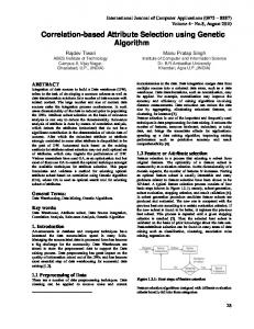
where Fit (f ) is the fitness function, cmax is the maximum estimate of the objective score, and f is the objective function value. The value of cmax is critical for ensuring that Fit (f ) is non-negative; otherwise, the problem may appear in the selection stage of the GA. According to the estimation of Equation (5), the value of cmax is 2. 4. Implementation of the Proposed Method Before the selection operation, operating units are extracted from the map dataset based on the “divide and conquer” principle. The selection is then carried out for each unit independently. Selection starts with the preprocessing procedure including building enlargement, local displacement,


11 of 23

conflict detection, and attribute enrichment. Then, the GA is employed to obtain the best solution. A flowchart of the selection process is given in Figure 10. ISPRS Int. J. Geo-Inf. 2017, 6, 271 11 of 23

Figure 10. Buildings selection procedure.

Figure 10. Buildings selection procedure.

4.1. Extraction of Selection Units

4.1. Extraction of Selection Units

First, selection units are extracted from the whole map. For this approach, a selection unit is a

First, units are extracted from whole map. in For this approach, a conflict selection unit is naturalselection group including a set of buildings andthe roads. Buildings a specific unit do not with buildings inincluding other units,a and thus they canand be treated in the Similar ideas of with a natural group set of buildings roads.together Buildings in ageneralization. specific unit do not conflict data partitioning haveand beenthus studied In thesetogether studies, the road network was used as aideas buildings in other units, they[8,25,30]. can be treated in the generalization. Similar framework to define the partition. Since roads in rural areas are not always enclosed, a new method of data partitioning have been studied [8,25,30]. In these studies, the road network was used as to extract selection units is necessary. a framework to define the partition. Since roads in rural areas are not always enclosed, a new method To derive suitable selection units, a polygon buffering approach is adopted based on the work to extract selection units is necessary. of Boffet [48]. This method was originally used to identify different types of settlements such as To derive suitable selectionand units, a polygon buffering approach isused adopted the work of major cities, towns, villages, hamlets. The values of the parameters belowbased are seton according Boffetto[48]. This method was originally used to identify different types of settlements such the experiments conducted by Boffet [48]. The main steps of the extraction process, as shownasinmajor cities,Figure towns, and hamlets. The values of thewith parameters below areassign set according 11,villages, are: (1) conducting a buffering operation 25 m as used the radius and a bufferedto the experiments conducted [48]. The mainbuffer steps areas of theinto extraction process, as shown in Figure area to each building;by (2)Boffet merging overlapping several large polygons that cover all 11, theconducting buildings; (3)a calculating the area of each polygons with areasaless than 20area ha can are: (1) buffering operation withpolygon, 25 m as and the radius and assign buffered to each be termed as rural settlements; and (4) selecting polygons for rural settlements, and overlaying them building; (2) merging overlapping buffer areas into several large polygons that cover all the buildings; with the building roadpolygon, layers. Buildings and roads the20 same polygon together (3) calculating the areaand of each and polygons withfalling areas within less than ha can be termed as rural form a selection unit. settlements; and (4) selecting polygons for rural settlements, and overlaying them with the building Note that not all selection units need to use the GA to perform the selection. For a unit with 10 and road layers. Buildings and roads falling within the same polygon together form a selection unit. or fewer buildings, the selection can be carried out directly according to a sequencing rule such as Note thatofnot selection units need to use the GA to perform the selection. For a unit with 10 or the sizes the all buildings. fewer buildings, the selection can be carried out directly according to a sequencing rule such as the sizes of the buildings.


12 of 23


12 of 23


12 of 23

Figure 11. Extraction selectionunits: units: (a) (a) building (b)(b) merging of buffered polygons; Figure 11. Extraction of of selection buildingbuffering; buffering; merging of buffered polygons; (c) conducting an overlap with roads; (d) conducting an overlap with buildings; (e) assigning (c) conducting an overlap with roads; (d) conducting an overlap with buildings; (e) assigning buildings buildings and roads to form selection units. and roads to form selection units.

4.2. Building Enlargement

4.2. Building Enlargement

To enforce the constraints of units: minimum size, buffering; small buildings should be enlarged before Figure 11. Extraction of selection (a) building (b) merging of buffered polygons; selection. If enlargement occurs after selection, the expansion of building size may lead to To enforce the constraints of minimum size, small buildings should be enlarged before selection. (c) conducting an overlap with roads; (d) conducting an overlap with buildings; (e) assigning new conflicts. According to the National Administration of Surveying [43], the rules for enlargement of buildings and roads to form selectionthe units. If enlargement occurs after selection, expansion of building size may lead to new conflicts. individual buildings at scales of 1:25,000 and 1:50,000 can be determined as follows. According to the National Administration of Surveying [43], the rules for enlargement of individual 4.2. Building Enlargement buildings at scales of graphic 1:25,000length and 1:50,000 can width be determined as follows. Rule 1. If the and graphic of a building are less than 0.7 mm and 0.5 mm, To enforce constraints of minimum small buildings be enlarged before respectively, thenthe replace the building with asize, predefined symbol ofshould the appropriate size and Rule 1. If the Ifgraphic lengthoccurs and graphic widththe of expansion a buildingofare less than 0.5 mm, selection. enlargement after selection, building size 0.7 maymm leadand to new orientation. respectively, then replace building withofthan aSurveying predefined the appropriate conflicts. According to the National Administration thegraphic rulesoffor enlargement of size Rule 2. If the graphic length ofthe a building is larger 0.7 mm,[43], butsymbol its width is less than individual buildings scales of 1:25,000 and can be determined as follows. 0.5 mm, then expandatits symbol width to 0.51:50,000 mm. Similarly, if the graphic width of a building is and orientation. larger thangraphic 0.5 mm, but its graphic length is less than 0.7than mm, 0.7 thenmm, expand its symbol length to 0.7ismm. Rule 2. IfRule the length of a building is larger graphic width less than 1. If the graphic length and graphic width of a building arebut lessits than 0.7 mm and 0.5 mm, Rule 3. If the graphic length and graphic width of a building are larger than 0.7 mm and 0.5amm, 0.5 mm, then width mm. Similarly, graphic width size of building respectively, then expand replace its thesymbol building withtoa 0.5 predefined symbolifofthethe appropriate and respectively, then represent them with their original outline. orientation. is larger than 0.5 mm, but its graphic length is less than 0.7 mm, then expand its symbol length Rule 2. If the of graphic length of is a building larger 12. than 0.7prerequisite mm, but its for graphic widthrules is less schematic the three rules shown inisFigure The the above is than that toA 0.7 mm. 0.5 mm, then expand its symbol width to 0.5 mm. Similarly, if the graphic width of a building is mm, the building is rectangular default. However, buildings are rectangles in the Rule 3. If the graphic lengthby and graphic widthnot of all a building arerepresented larger thanas0.7 mm and 0.5 larger than 0.5 mm, but its graphic length is less than 0.7 mm, then expand its symbol length to 0.7 mm. map. For non-rectangular buildings, in addition to expanding their size, shape simplification may respectively, then represent them with their original outline. Rulerequired. 3. If the graphic lengththat andrural graphic width ofare a building larger than 0.7itmm and 0.5 mm, also be Considering buildings usually are relatively small, is rarely worth respectively, then represent them is with original outline. simplifying their shapes. antheir enlargement method proposed that the smallest A schematic of the threeTherefore, rules shown in Figure 12. Theisprerequisite forutilizes the above rules is that minimum bounding rectangle (SMBR). On the premise of expanding the size, this method can A schematic of the three rules is shown in Figure prerequisite for the above as rules is that the building is rectangular by default. However, not12. allThe buildings are represented rectangles in simplify the shape simultaneously. As the smallest rectangle that includes the whole building, the the building is rectangular by buildings, default. However, not all to buildings are represented rectangles in the the map. For non-rectangular in addition expanding their size,asshape simplification SMBR is fitted because it can maximally approximate the size and shape of the original building. Forrequired. non-rectangular buildings, addition to expanding their relatively size, shapesmall, simplification mayworth may map. also be Considering thatinrural buildings are usually it is rarely also be required. Considering that rural buildings are usually relatively small, it is rarely worth simplifying their shapes. Therefore, an enlargement method is proposed that utilizes the smallest simplifying their shapes. Therefore, an enlargement method is proposed that utilizes the smallest minimum bounding rectangle (SMBR). On the premise of expanding the size, this method can simplify minimum bounding rectangle (SMBR). On the premise of expanding the size, this method can the shape simultaneously. As the smallest rectangle that includes the whole building, the SMBR is simplify the shape simultaneously. As the smallest rectangle that includes the whole building, the fittedSMBR because it can maximally approximate the size and shape the original building. is fitted because it can maximally approximate the size andofshape of the original building.

Figure 12. Three rules for enlargement of individual buildings at scales of 1:25,000 and 1:50,000.



ISPRS J. Geo-Inf. Geo-Inf. 2017, 2017, 6, 6, 271 271 ISPRS Int. Int. J. ISPRS Int. J. Geo-Inf. 2017, 6, 271

13 of of 23 23 13 13 of 23

In the Cartesian coordinate system with the east–west direction as the horizontal axis, the direction as the horizontal axis,axis, the In the the Cartesian Cartesian coordinate coordinatesystem systemwith withthetheeast–west east–west direction as the horizontal enlargement begins by generating an SMBR for each building. Using the center of gravity as the enlargement begins by generating an SMBR for for eacheach building. Using the center of gravity as the the enlargement begins by generating an SMBR building. Using the center of gravity as anchor point, the SMBR is then rotated so that its long axis is horizontal. By comparing the length anchor point, thethe SMBR is then rotated soso that the anchor point, SMBR is then rotated thatitsitslong longaxis axisisishorizontal. horizontal.By By comparing comparing the length and width of the rotated graphic symbols with the predefined thresholds, a simple geometric widthofof rotated graphic symbols with the predefined thresholds, a simple expansion geometric and width thethe rotated graphic symbols with the predefined thresholds, a simple geometric expansion is performed in the horizontal and vertical directions. Finally, the rotation is implemented expansion is performed in the horizontal and vertical directions. Finally, theisrotation is implemented is performed in the horizontal and vertical directions. Finally, the rotation implemented again for again for each enlarged SMBR to return the long axis to its original orientation. Then, the original againenlarged for each SMBR enlarged SMBR the to return the to long axis to its original orientation. Then, the original each to return long axis its original orientation. Then, the original buildings buildings can be replaced by these enlarged graphic symbols. Figure 13 illustrates the process buildings can be by these enlarged graphic symbols. Figure illustrates the process can be replaced by replaced these enlarged graphic symbols. Figure 13 illustrates the13 process consisting of two consisting of two rotations and one geometric change. consisting of two rotations and one geometric change. rotations and one geometric change.

Figure 13. Building enlargement process: (a) original buildings; (b) SMBRs; (c) first rotation; 13.Building Building enlargement process: (a) original buildings; (b) SMBRs; (c) first(d) rotation; Figure 13. enlargement process: (a) original buildings; (b) SMBRs; (c) first rotation; simple (d) simple geometric transformation; (e) second rotation; (f) buildings after enlargement compared to (d) simple geometric transformation; (e)rotation; second rotation; (f) buildings after enlargement compared to geometric transformation; (e) second (f) buildings after enlargement compared to their their initial states. their initial initial states.states.

4.3. Local Displacement 4.3. Local Displacement After enlargement of the building size, the feature symbols that are originally separated from After enlargement of the building size, the feature symbols that are originally originally separated from each other may overlap. To maintain the topological relationship among the buildings and their overlap. To each other may overlap. To maintain the topological relationship among the buildings and their surrounding roads, the overlap needs to be removed. Since roads are more important than buildings surrounding roads, the overlap needs to be removed. Since roads are more important than buildings in maps [49], the correct topological relationship is retained by displacing the overlapping buildings. in maps [49], the correct topological relationship is retained by displacing the overlapping buildings. According to the positional relationship, overlapping buildings can be classified into two types: According to the positional relationship, overlapping buildings can be classified into two types: the corner type (C-type) and the edge type (E-type) (see Figure 14). Definitions for the buildings of the corner type (C-type) and the edge type type (E-type) (E-type) (see Figure Figure 14). 14). Definitions for the buildings of these two types are as follows: are as as follows: follows: these two types are • A C-type building is one that is located at a road corner and overlaps at least one of the roads. A C-type C-type building building is is one one that that is is located located at at aa road road corner corner and and overlaps overlaps at at least least one oneof of the theroads. roads. •• A • An E-type building is one that is located on one side of the road and only overlaps one of the •• An E-type building is one that is located on one side of the road and only overlaps one the An E-type building is one that is located on one side of the road and only overlaps one of the of roads. roads. roads.

Two types of buildings that overlap surrounding roads. Figure 14. Two Figure 14. Two types of buildings that overlap surrounding roads.

ISPRS Int. J. Geo-Inf. 2017, 6, 271 ISPRS Int. J. Geo-Inf. 2017, 6, 271

14 of 23 14 of 23

For C-type vector. ISPRSaInt. J. Geo-Inf.building, 2017, 6, 271 buffering technology is used to determine its displacement 14 of 23 building, buffering technology is determine displacement vector. In In Figure For 15a,a aC-type buffering operation is conducted forused the tonearby roaditsedges. The buffer radius is Figure 15a, a buffering operation is conducted for the nearby road edges. The buffer radius is set to For a C-type building, buffering technology is used to determine its displacement vector. In set to be half the larger diagonal length of the enlarged building. After that, the overlapping buffers be half 15a, the larger diagonal lengthisofconducted the enlarged building. After theThe overlapping buffers will Figure a buffering operation nearby roadthat, edges. buffer radius is set to then will form an intersection (marked as a star) on for thethe inside corner. The displacement vector can form anthe intersection (marked as a of star) the inside corner.After The that, displacement vector can thenwill be be half larger diagonal length theon enlarged building. the overlapping buffers be determined with the center of gravity of the building as the start point and the intersection as determined with the (marked center of as gravity thethe building as the start and the vector intersection as the form an intersection a star)ofon inside corner. The point displacement can then be the end point. Figure15b 15bshows shows that, an E-type building, the displacement direction end point. Figure forfor anthe E-type building, displacement direction is set as to is beset to determined with the center ofthat, gravity of building as thethe start point and the intersection the be perpendicular to road. The displacement magnitude is the d1direction and d2 , is where 1 is the perpendicular to the the The displacement magnitude the sumsum of dof 1 and d2, where d1 istodthe end point. Figure 15broad. shows that, for an E-type building,isthe displacement set be nearest distance from the original building the road,and and isthethe distance that the nearest distance the original building to to magnitude the road, d2d2is maximum perpendicular tofrom the road. The displacement is the sum of dmaximum 1 and d2distance , where dthat 1 is the enlarged building covers the road. avoid of constraint C4, is necessary to check enlarged building covers road.To To avoidthe the violation constraint it isitnecessary to check the the nearest distance from thethe original building to violation the road,of and d2 is theC4, maximum distance that displacement magnitude before a building is displaced. Once the displacement magnitude exceeds displacement magnitude before a building is displaced. Once the displacement magnitude enlarged building covers the road. To avoid the violation of constraint C4, it is necessary to check exceeds the 0.5 mm, the building should removed instead of being beingOnce displaced. displacement magnitude before a building is displaced. the displacement magnitude exceeds 0.5 mm, the building should bebe removed instead of displaced. 0.5 mm, the building should be removed instead of being displaced.

Figure 15. Determination of the building displacement vector for: (a) a C-type building; (b) an E-type Figure 15. Determination of the building displacement vector for: (a) a C-type building; (b) an E-type building. building. Figure 15. Determination of the building displacement vector for: (a) a C-type building; (b) an E-type building.

4.4. Conflict Detection among Buildings 4.4. Conflict Detection among Buildings

4.4. Conflict Detection Buildings Spatial conflicts occuramong whenwhen the distance between two two buildings is shorter thanthan the minimum distance Spatial conflicts occur the distance between buildings is shorter the minimum distance oroccur whenoverlap buildings overlap This paper the buffer-based approach threshold, or threshold, when buildings each other.each Thisother. paper uses the uses buffer-based approach [6,49,50] to Spatial conflicts when the distance between two buildings is shorter than the minimum to (see detect conflicts (see Figure 16). Inaeach thisother. method, buffer area isbuffer-based constructed for each distance threshold, or when overlap This uses thefor approach detect[6,49,50] conflicts Figure 16). buildings In this method, buffer area isapaper constructed each building with half building with half threshold the minimum distance as of theone radius. Ifarea theoverlaps buffer of onethat building [6,49,50] to detect conflicts (see Figure 16).threshold this method, a buffer is constructed for of each the minimum distance as the radius. IfInthe buffer building with another overlaps with that of another building, there is a conflict between the two buildings. building with half the minimum distance threshold as the radius. If the buffer of one building building, there is a conflict between the two buildings. overlaps with that of another building, there is a conflict between the two buildings.

Figure 16. The buffer-based approach for detecting conflicts. r’ is half the minimum distance threshold detecting conflicts. Figure 16.for The buffer-based approach for detecting conflicts. r’ is the halfminimum the minimum distance Figure 16. The buffer-based approach for detecting conflicts. r’ is half distance threshold threshold for detecting conflicts. for detecting conflicts. Conflicting blocks are taken into account in encoding, crossover, and mutation. To avoid repetitive detection of spatial conflicts to speed the running speed ofand the mutation. GA, a conflict Conflicting blocks are taken intoand account in up encoding, crossover, To index avoid Conflicting blocks are taken into account in encoding, crossover, and mutation. To avoid repetitive list after building enlargement and local displacement generated. The conflict indexa mainly repetitive detection of spatial conflicts and to speed upisthe running speed of the GA, conflict stores index detection of spatial conflicts and to speed up the running speed of the GA, a conflict index list conflicting block information each building. Therefore, in the selection process, oncemainly a building is after list after building enlargementfor and local displacement is generated. The conflict index stores processed, all buildings that conflict it can be easily searched. building enlargement and local displacement is generated. The index mainly conflicting conflicting block information for eachwith building. Therefore, in theconflict selection process, oncestores a building is

all buildings conflictTherefore, with it canin bethe easily searched. blockprocessed, information for each that building. selection process, once a building is processed, all buildings that conflict with it can be easily searched.


15 of 23

4.5. Enrichment of Geometric Attributes This subsection aims to identify specific buildings on the source map that are important to retain. According to the previous description, it is necessary to identify three types of important buildings. (1)

(2)

(3)

A type I building is determined by simple area calculation and comparison to the minimum size threshold. According to the National Administration of Surveying [43], buildings with an area of more than 0.35 mm2 are considered to be of this type. A type II building is identified on the basis of detecting the proximity relationship among buildings and roads. Before performing the GA on a selection unit, a proximity graph is constructed using the method proposed by Liu et al. [51]. It is then possible to obtain information as to whether a building is adjacent to a road and how close it is. Utilizing the information, a building that is adjacent to two or more roads and whose proximity distance to each road is less than a certain threshold (e.g., 15 m) can be defined as a type II building. To identify a type III building, the boundary of a settlement should be defined first. A boundary deriving method proposed by Yan and Weibel [17] is adopted after converting the building group to a point cluster. The buildings that overlap the generated boundary are called the boundary buildings. A type III building can be derived from these boundary buildings by performing a line reduction algorithm on the boundary line. The Douglas–Peucker algorithm [52] is preferred because it keeps all the key points that make up the basic shape of a line and removes the other points. The simplified tolerance in the algorithm is set to 25 m by experiment. The buildings corresponding to the points retained on the simplified line will be type III buildings.

4.6. Selection Based on the GA Before running the GA, the must-be-selected buildings should be extracted from the three types of important buildings and the building alignment. Then, the must-be-discarded buildings can be easily determined using the generated conflict index. 4.6.1. Initialization The GA begins with initialization, which generates the first population. The process of initializing a chromosome can be summarized as: (1) (2) (3) (4)

Mark all genes as ‘free’; Assign the gene values corresponding with the must-be-selected buildings as 1 s and mark these genes as ‘fixed’; Assign the gene values corresponding with the must-be-discarded buildings as 0 s and mark these genes as ‘fixed’; Repeat the following steps until the number of genes assigned as 1 s reaches the target selection number or all the genes are marked as ‘fixed’; (4.1) (4.2)

Randomly select a ‘free’ building B and assign its gene as 1, then mark the gene as ‘fixed’; Identify ‘free’ buildings from CB(B), assign the corresponding genes as 0 s and mark these genes as ‘fixed’;

To determine the target selection number, Töpfer’s radical law [37] can be applied: Nt = Ns

p

Ms /Mt ,

(7)

where Nt is the number of buildings in the target map, Ns is the number of buildings in the source map, Ms is the denominator of the source scale, and Mt is the denominator of the target scale. Through the above process, initialization of a chromosome is completed. A population often contains a set of chromosomes. In general, an initial population with a large size can handle more


16 of 23

solutions at the same time, making it easier to find the global optimal solution. But the disadvantage is that it increases the time of each iteration. The general value of population size Psize ranges from 20 to 100. In this paper, the population sizes are set to 50 (at 1:25,000) and 150 (at 1:50,000), which have been determined through experimental testing. 4.6.2. Selection, Crossover, and Mutation After the population is initialized, the GA makes use of crossover and mutation to evolve new solutions. The first step is to select appropriate individuals for the genetic operators. There are several selection operations available, and the one used here is the fitness proportionate selection, because it makes the GA robust. The basic idea is that the probability for each individual to be selected is proportional to its fitness value. The way to perform crossover and mutation has been discussed in Section 3.3, but how to set the crossover probability Pc and mutation probability Pm remains a problem. The crossover probability indicates the probability that crossover operation will occur on two selected parents. If the value is set too high, individuals with high fitness can easily be destroyed. However, too small a crossover probability will slow down the search process. The mutation probability determines the probability that a gene value in an individual is altered. The GA becomes a random search algorithm when the mutation probability is set too high, since the gene information is easy to change. Too low a mutation probability will reduce the local search capability of the algorithm. In this paper, the crossover probability is set to 0.8, and the mutation probability is set to 0.1, which have been determined through experimental testing. 4.6.3. Iteration and the Elite Retention Strategy After crossover and mutation, the children will replace the parent chromosomes in the initial population. To avoid destroying an excellent individual in the evolutionary process, the elite retention strategy [53] is introduced into the GA. The idea of the strategy in this paper is that the best individual of the previous generation can be directly copied to the next generation. This excellent individual, together with other children, produces a new population. The GA then starts the next evolution based on the new population. Through multiple iterations, the individual with the highest fitness value is obtained as the selection results. The iterative process terminates when the algorithm reaches the maximum generation Gm , where Gm is set using an experimentally determined threshold, namely 30 (at 1:25,000) and 50 (at 1:50,000). 5. Results and Analysis 5.1. Experimental Results To validate the effectiveness of the approach, two selection units were chosen to carry out experiments on. They were extracted from the topographic dataset of Caidian District, Wuhan City, China. The original scale of the topographic map was 1:10,000, and the target scales were 1:25,000 and 1:50,000. For both selection units, the symbol width of roads was set to 0.2 mm and the outline width of buildings was set to 0.1 mm. The road was properly selected according to the scale changes. The proposed approach was programmed using C# and ArcGIS Engine, and the tests were implemented on a PC with Windows 7 OS and Intel® Core™ i5-4460 CPU (3.20 GHz). Figure 17 shows the two selection units. Unit A contains 157 buildings and unit B contains 204 buildings. Figures 18 and 19 demonstrate the results of unit A and a comparison of its states before and after selection. As shown in Figures 17–19, there are two identified building alignments plotted with blue lines in selection unit A. The experimental results for unit B are shown in Figures 20 and 21. A preliminary conclusion can be obtained through visual evaluation that the resultant map is more legible and the distribution characteristic is well maintained. Detailed statistical information is given in Tables 1–3 below.


17 of 23


17 of 23 17 of 23

Figure 17. Two test datasets: (a) selection unit A and (b) selection unit B. Figure 17. Two test datasets: (a) selection unit A and (b) selection unit B. Figure 17. Two test datasets: (a) selection unit A and (b) selection unit B.

Figure 18. Test results of selection unit A: (a) visual reduction without selection (1:25,000), (b) selection the GA (1:25,000), (c) selection results (1:25,000), enlarged (b) to selection 1:10,000 result from Figure 18. Testresult resultsusing of selection unit A: (a) visual and reduction without selection Figure 18. Test results of selection unit A: (a) visual reduction without selection (1:25,000), 1:25,000. using the GA (1:25,000), and (c) selection results enlarged to 1:10,000 from 1:25,000. (b) selection result using the GA (1:25,000), and (c) selection results enlarged to 1:10,000 from 1:25,000.

19.Test Test results of selection unit A: reduction (a) visual reduction without selection (1:50,000), Figure 19. results of selection unit A: (a) visual without selection (1:50,000), (b) selection result (b) selection using the(c)GA (1:50,000), (c) selection result enlarged to 1:10,000 from 1:50,000. using the GA result (1:50,000), and selection resultand enlarged to 1:10,000 from 1:50,000. Figure 19. Test results of selection unit A: (a) visual reduction without selection (1:50,000), (b) selection result using the GA (1:50,000), and (c) selection result enlarged to 1:10,000 from 1:50,000.

J. Geo-Inf. 6, 271 ISPRS ISPRS Int. J. Int. Geo-Inf. 2017,2017, 6, 271

18 of 23 18 of 23 18 of 23


Figure 20.results Test results of selection B: reduction (a) visualwithout reduction without selection Figure 20. Test of selection unit B: (a)unit visual selection (1:25,000), (b) (1:25,000), selection result Figure 20. Test results of selection unit B: (a) visual reduction without selection (1:25,000), selection result using theselection GA (1:25,000), and (c) selection resultfrom enlarged to 1:10,000 from 1:25,000. using(b) the GA (1:25,000), and (c) result enlarged to 1:10,000 1:25,000. (b) selection result using the GA (1:25,000), and (c) selection result enlarged to 1:10,000 from 1:25,000.

Figure 21. Test of selection unit B: (a)unit visual selection (1:50,000), (b) (1:50,000), selection result Figure 21.results Test results of selection B: reduction (a) visualwithout reduction without selection Figure 21. Test results of selection unit B: (a) visual reduction without selection (1:50,000), result using theselection GA (1:50,000), (c) selection resultfrom enlarged to 1:10,000 from 1:50,000. using(b) theselection GA (1:50,000), and (c) resultand enlarged to 1:10,000 1:50,000. (b) selection result using the GA (1:50,000), and (c) selection result enlarged to 1:10,000 from 1:50,000. Table Statisticalanalysis analysis of Table 1. 1. Statistical ofthe theGA GAresults. results. Table 1. Statistical analysis of the GA results. Selection Selection

Unit Selection Unit Unit A A

A B

B B

Scale Scale Scale 1:25,000 1:25,000 1:50,000 1:50,000 1:25,000 1:25,000 1:25,000 1:50,000 1:50,000 1:50,000

1:25,000 1:50,000

Initial Initial

Final Final

Estimated Building Estimated Building

0 0 0 0 0 0

70 99 129 129 70 91

Conflicts Conflicts Estimated Number Initial Final Building Conflicts Conflicts Number 170 0 99 Conflicts Conflicts Number 170 0 99 642

642 170132 132 642637 637

0 0

70

91

Resultant Execution Resultant Execution Building Number (s) Resultant BuildingTime Building Number TimeExecution (s) 79 66Time (s) Number 79 66 37 136 37 136 125 79 108 66 125 108 53 37 193 136 53 193

132 0 129 2. Magnitude of distribution changes. 637Table 0 91 range Table 2. Magnitude of distribution range changes.

125 53

108 193

Selection Unit Unit A Unit B Selection Unit Unit A Unit B Scale 1:25,000 1:50,000 1:25,000 1:50,000 Table 2. Magnitude of distribution changes. Scale 1:25,000 1:50,000 range 1:25,000 1:50,000 Ratio of changes (%) 3.38 11.24 1.85 9.99 Ratio of changes (%) 3.38 11.24 1.85 9.99

Selection Unit

Unit A

Unit B

Table 3. Density information at different scales. information at different1:25,000 scales. Scale Table 3. Density 1:25,000 1:50,000 1:50,000 Selection Unit Unit A B Ratio of changes 3.38 11.24 1.85Unit 9.99 Selection Unit (%) Unit A Unit B Scale 1:10,000 1:25,000 1:50,000 1:10,000 1:25,000 1:50,000 Scale 1:10,000 1:25,000 1:50,000 1:10,000 1:25,000 1:50,000 Building density 0.112 0.122 0.206 0.126 0.149 0.212 Building density 0.112 0.206at different 0.126 scales. 0.149 0.212 Table 3. Density0.122 information

Selection Unit Scale Building density

Unit A 1:10,000 0.112

1:25,000 0.122

Unit B 1:50,000 0.206

1:10,000 0.126

1:25,000 0.149

1:50,000 0.212


19 of 23

5.2. Analysis The goal of building selection is to remove spatial conflicts caused by scale reduction under related cartographic constraints. Therefore, the quality of the selection results can be assessed by determining whether these constraints have been satisfied. 5.2.1. Local Constraints ISPRS Int. J. Geo-Inf. 2017, 6, 271

19 of 23

In this approach, the size constraint was enforced by building enlargement. It is advisable to give 5.2. Analysis a higher priority to this constraint because it generally has an impact on other constraints. For example, The goal building selection is towill remove spatial conflicts causedwhich by scale reduction the distance among theofenlarged buildings inevitably be reduced, may cause under violation of the cartographic constraints. Therefore, the quality of the selection results can be assessed by separationrelated constraint. Using the strategy that the enlargement comes first can avoid potential conflicts. determining whether these constraints have been satisfied. The enlargement method used in this paper adopts the SMBR. Therefore, it has the beneficial effects of 5.2.1.constraints Local Constraints satisfying the on granularity and squareness at the same time. In addition, the two rotations guarantee that In the resultant maintain original mainenlargement. directions.ItRespecting this approach,buildings the size constraint was their enforced by building is advisable tothese give aconstraints higher priority to this constraint it generally has legible. an impactAfter on other constraints. For the the spatial ensures that the buildings retained inbecause the target map are enlargement, toexample, maintain distance among the enlarged will inevitably be reduced, which may of the displaced relationship among the building andbuildings other features, the building symbols maycause needviolation to be locally separation constraint. Using the strategy that the enlargement comes first can avoid potential conflicts. during theThe selection process. To ensure positional accuracy, the displacements have been purposefully enlargement method used in this paper adopts the SMBR. Therefore, it has the beneficial effects of limited within a specific range (e.g., 0.5 mm). satisfying the constraints on granularity and squareness at the same time. In addition, the two rotations guarantee that the resultant buildings maintain their original main directions. Respecting The separation constraint is evaluated by measuring the number of spatial conflicts.these As shown in constraints ensures that the buildings retained in the target map are legible. After enlargement, to Table 1, initial conflicts and final conflicts refer to the conflicts among the enlarged buildings at the maintain the spatial relationship among the building and other features, the building symbols may target scale before and after selection. It can be seen that all the conflicts among the buildings have need to be locally displaced during the selection process. To ensure positional accuracy, the been completely resolved selection. However, thea specific number of selected buildings does not strictly displacements haveafter been purposefully limited within range (e.g., 0.5 mm). constraint is evaluated measuring the number of spatial conflicts. shown building correspond to The theseparation radical law, especially at theby1:50,000 scale. The reason is that the As enlarged Table 1, initial conflicts when and final conflicts to the conflicts among the enlarged buildings at the size is far frominthe initial geometry the scale refer is reduced to 1:50,000. This greatly increases the target scale before and after selection. It can be seen that all the conflicts among the buildings of the conflicting block of each building and further reduces the number of optional buildings when have been completely resolved after selection. However, the number of selected buildings does not encoding.strictly Taking this situation into law, account, theatinitialization ofThe a chromosome been set to be correspond to the radical especially the 1:50,000 scale. reason is that thehas enlarged far the frombuildings the initial geometry when theeven scale is to 1:50,000. This greatly increases stopped asbuilding long asisall are processed, if reduced the estimated building number has not been the size of the conflicting block of each building and further reduces the number of optional reached. In this way, building conflicts can be avoided as much as possible. buildings when encoding. Taking this situation into account, the initialization of a chromosome has The current method satisfies the functionality constraint by enriching the geometry attributes and been set to be stopped as long as all the buildings are processed, even if the estimated building fixing important buildings when encoding. identified must-be-selected buildings number has not been reached. In this way, The building conflicts can be avoided as much as possible.for two units The current satisfies the functionality constraintare by enriching thetypes geometry andbuildings, are shown in Figures 22method and 23. Among these buildings the three of attributes important fixing important buildings that whenshould encoding. identified buildings for Some two units are whilst others are the buildings beThe kept in themust-be-selected identified alignments. buildings may shown in Figures 22 and 23. Among these buildings are the three types of important buildings, whilst belong to more than one type at the same time. All these buildings are contained in the final solution. others are the buildings that should be kept in the identified alignments. Some buildings may belong As shown,to the at these 1:25,000 are are more than in those at 1:50,000. moremust-be-selected than one type at the buildings same time. All buildings contained the final solution. As The main must-be-selected buildings at 1:25,000 are more at 1:50,000.asThe main difference differenceshown, lies inthe the type I buildings. A building that canthan bethose recognized type I on a 1:50,000 map lies in the type I buildings. A2building that can be recognized as type I on a 1:50,000 map requires an requires an area of at least 2875 m in the real world. Such a large building is very rare in rural areas. area of at least 875 m in the real world. Such a large building is very rare in rural areas. In this paper, In this paper, the semantic attributes of buildings are lacking. As for a dataset with rich semantic the semantic attributes of buildings are lacking. As for a dataset with rich semantic attributes, the attributes,approach the approach can extended be easilytoextended tosemantically include these semantically can be easily include these important buildings. important buildings.

22. Must-be-selected buildings in in selection unitunit A when the target is: (a)scale 1:25,000, Figure 22.Figure Must-be-selected buildings selection A when thescale target is: and (a) 1:25,000, (b) 1:50,000. The green dashed line is the simplified boundary line. and (b) 1:50,000. The green dashed line is the simplified boundary line.


20 of 23


20 of 23 20 of 23

23. Must-be-selected buildings in selection unit BB when the the target scale is: (a)scale 1:25,000, Figure 23.Figure Must-be-selected buildings inin selection unit when target scale is: (a) 1:25,000, and Must-be-selected buildings selection unit B when the target is: and (a) 1:25,000, (b) 1:50,000. The green dashed line is the simplified boundary line. (b) 1:50,000. The green dashed line is theissimplified boundary line.line. and (b) 1:50,000. The green dashed line the simplified boundary

5.2.2. Contextual Constraint of Spatial Relationships and Patterns

Constraint of Spatial 5.2.2. Contextual Relationships andresults Patterns An important indicator to assess the generalization is whether building alignments are preserved. To satisfy this constraint, the building alignments must first be identified. Multiple An important indicator to assess the generalization results is whether building alignments are studies have been undertaken by various researchers to detect buildings in alignment [11,25,38,42]. preserved.With Tosatisfy satisfyofthis constraint, the building alignments must first be identified. Multiple preserved. To constraint, building must first be identified. Multiple studies the aid this these methods,the these buildingalignments alignments are extracted automatically and then studiesbeen have beenin undertaken by various researchers to detect buildingsinin alignment alignment [11,25,38,42]. handled the algorithm. have undertaken by various researchers to detect buildings [11,25,38,42]. building alignments of selection unitalignments A in are Figures 17–19 are magnified for closer With the theaid aidofThe of these methods, these building are extracted automatically then With these methods, these building alignments extracted automatically and thenand handled observation in Figure 24. When the scale is reduced to 1:25,000, it is still possible to identify the handled in the algorithm. in the algorithm. alignments. In the 1:50,000 maps, the number of buildings in both alignments is reduced to 2. As the building alignment alignments ofcontain selection unit A in Figures are magnified for closer The building of selection in Figures 17–19 are17–19 magnified for closer observation recognizedalignments should atunit leastAthree buildings, the alignments are unrecognizable at observation in Figure 24. When the scale is reduced to 1:25,000, it is still possible to identify the It is found that whether the alignment constraint be satisfied is highly correlated the to two in Figure 1:50,000. 24. When the scale is reduced to 1:25,000, it can is still possible to identify alignments. factors: the number of aligned buildings and the degree of scale change. When the number of alignments. In maps, the 1:50,000 maps, of thebuildings number of in both is alignments 2. As the In the 1:50,000 the number in buildings both alignments reduced tois2.reduced As the to recognized buildings is relatively small, may be unrecognized at a the scalealignments of 1:25,000. On theunrecognizable contrary, recognizedaligned alignment should contain atitleast three buildings, are at alignment should contain at least three buildings, the alignments are unrecognizable at 1:50,000. alignments with a higher number of buildings may still be significant, even at 1:50,000. 1:50,000. It is found that whether the alignment constraint can be satisfied is highly correlated to two It is found that whether the alignment constraint can be satisfied is highly correlated to two factors: factors: the of number aligned and buildings andofthe degree of When scale the change. When the number of the number alignedofbuildings the degree scale change. number of aligned buildings aligned buildings small, it may at beaunrecognized at a scale of contrary, 1:25,000. alignments On the contrary, is relatively small,isitrelatively may be unrecognized scale of 1:25,000. On the with with aofhigher number buildings may still be at significant, aalignments higher number buildings mayof still be significant, even 1:50,000. even at 1:50,000.

Figure 24. Two alignments of selection unit A in detail. The pictures on the left are building alignments at the source map scale, the pictures in the middle are building alignments at 1:25,000, and the pictures on the right are building alignments at 1:50,000 (outlined shapes: original buildings, fully shaded shapes: selected buildings).

To evaluate the change of distribution range, the ratio between the area difference of the distribution range and the area of the initial distribution range was used. The smaller the ratio, the better the preservation of the distribution range. The results are shown in Table 2, where the

Figure 24. of selection unit unit A in detail. The pictures on the left building alignments 24.Two Twoalignments alignments of selection A in detail. The pictures onare the left are building at the sourceatmap themap pictures thepictures middle are building alignments at 1:25,000, and the pictures alignments the scale, source scale,inthe in the middle are building alignments at 1:25,000, on are building alignments at 1:50,000 (outlined shapes: original buildings, fully shaded andthe theright pictures on the right are building alignments at 1:50,000 (outlined shapes: original buildings, shapes: selected buildings). fully shaded shapes: selected buildings).

To evaluate evaluatethe the change of distribution thebetween ratio between the area difference of the To change of distribution range,range, the ratio the area difference of the distribution distribution range and the area of the initial distribution range was used. The smaller the ratio, range and the area of the initial distribution range was used. The smaller the ratio, the better the the better the preservation of the range. distribution range.are The results shown in Table 2, whereratio the preservation of the distribution The results shown in are Table 2, where the maximum of range changes is 11.24%. It can therefore be considered that the distribution range is well preserved.


21 of 23

According to Regnauld et al. [46], distribution density can be evaluated from the perspective of contrast of different units across a map. Table 3 illustrates the density information of the two selection units at different scales. As shown, the ordering of density values between the two units is consistent prior to and after selection. That is, unit B has a higher density than unit A at 1:10,000, and this situation still exists after selection. The conclusion can be drawn that the contrast among units of different density is well maintained. 6. Conclusions and Future Work Building selection is a process in which various factors interact with and restrict each other. This study has proposed an improved GA for automated building selection. The proposed algorithm is highly efficient as it takes into account a wide range of constraints while producing very satisfactory results. On the one hand, spatial conflicts among buildings have all been resolved after selection by considering conflicting blocks when performing the encoding and genetic operations. On the other hand, the spatial distribution characteristics are well maintained, as the contextual constraints have been introduced into the fitness function. The improved algorithm was found to be feasible for conflict resolution for rural buildings, especially when their overall density was too high to perform displacement. Future research will focus on collaborative generalization with other contextual operators, especially displacement. In this paper, the GA was mainly used to remove intra-feature conflicts. Inter-feature conflicts among buildings and their surrounding features, such as roads and rivers, have not been fully considered. These conflicts may be caused by scale reduction or the generalization operations of other features. For example, the symbolization, simplification, and displacement of roads may lead to spatial conflicts among roads and their adjacent buildings. Therefore, it is of great interest to collaborate the available generalization algorithms to resolve multiple cartographic conflicts. Acknowledgments: This research was supported in part by the National Natural Science Foundation of China (Grant No. 41471384, No. 41071289, and No. 41701537). Author Contributions: Lin Wang and Qingsheng Guo conceived and designed the experiments; Lin Wang and Yageng Sun performed the experiments; Lin Wang, Qingsheng Guo, and Zhiwei Wei analyzed the data; Yuangang Liu contributed reagents/materials/analysis tools; Lin Wang and Qingsheng Guo wrote the paper. Conflicts of Interest: The authors declare no conflict of interest.

References 1. 2. 3. 4. 5. 6. 7. 8. 9.

McMaster, R.B.; Shea, K.S. Generalization in digital cartography. In Spatial Data Handling; Association of American Geographers: Washington, DC, USA, 1992; pp. 6.1–6.18. Ruas, A.; Plazanet, C. Strategies for automated generalization. In Proceedings of the 7th International Symposium on Spatial Data Handling, Delft, The Netherlands, 12–16 August 1996. Brassel, K.E.; Weibel, R. A review and conceptual framework of automated map generalization. Int. J. Geogr. Inf. Syst. 1988, 2, 229–244. [CrossRef] Mackaness, W.A. An algorithm for conflict identification and feature displacement in automated map generalization. Cartogr. Geogr. Inf. Syst. 1994, 21, 219–232. [CrossRef] Ruas, A. A method for building displacement in automated map generalisation. Int. J. Geogr. Inf. Syst. 1998, 12, 789–803. [CrossRef] Lonergan, M.; Jones, C.B. An iterative displacement method for conflict resolution in map generalization. Algorithmica 2001, 30, 287–301. [CrossRef] Harrie, L.; Sarjakoski, T. Simultaneous graphic generalization of vector data sets. GeoInformatica 2002, 6, 233–261. [CrossRef] Bader, M.; Barrault, M.; Weibel, R. Building displacement over a ductile truss. Int. J. Geogr. Inf. Sci. 2005, 19, 915–936. [CrossRef] Ai, T.; Zhang, X.; Zhou, Q.; Yang, M. A vector field model to handle the displacement of multiple conflicts in building generalization. Int. J. Geogr. Inf. Sci. 2015, 29, 1310–1331. [CrossRef]


10.

11. 12. 13. 14.

15.

16.

17. 18. 19. 20. 21. 22. 23. 24. 25. 26. 27. 28. 29. 30. 31. 32. 33.

22 of 23

Ai, T.; Zhang, X. The aggregation of urban building clusters based on the skeleton partitioning of gap space. In The European Information Society; Fabrikant, S., Wachowicz, M., Eds.; Springer: Aalborg, Denmark, 2007; pp. 153–170. Regnauld, N. Contextual building typification in automated map generalization. Algorithmica 2001, 30, 312–333. [CrossRef] Yan, H.; Weibel, R.; Yang, B. A multi-parameter approach to automated building grouping and generalization. Geoinformatica 2008, 12, 73–89. [CrossRef] Kadmon, N. Automated selection of settlements in map generalisation. Cartogr. J. 1972, 9, 93–98. [CrossRef] Langran, G.E.; Poiker, T.K. Integration of name selection and name placement. In Proceedings of the 2nd International Symposium on Spatial Data Handling, Seattle, WA, USA, 5–10 July 1986; International Geographical Union and International Cartographic Association: Seattle, WA, USA, 1986; pp. 50–64. Ai, T.; Liu, Y. Analysis and simplification of point cluster based on delaunay triangulation model. In Advances in Spatial Analysis and Decision Making; Li, Z., Zhou, Q., Kainz, W., Eds.; Taylor & Francis: London, UK, 2003; pp. 9–18. Qian, H.; Meng, L. Polarization transformation as an algorithm for automatic generalization and quality assessment. In Proceedings of the SPIE 6751, Geoinformatics 2007: Cartographic Theory and Models, Nanjing, China, 25–27 May 2007; Li, M., Wang, J., Eds.; The International Society for Optical Engineering: Nanjing, China, 2007; Volume 67510Y. Yan, H.; Weibel, R. An algorithm for point cluster generalization based on the voronoi diagram. Comput. Geosci. 2008, 34, 939–954. [CrossRef] Peters, S. Quadtree-and octree-based approach for point data selection in 2D or 3D. Ann. GIS 2013, 19, 37–44. [CrossRef] Yan, H.; Li, J. An approach to simplifying point features on maps using the multiplicative weighted voronoi diagram. J. Spat. Sci. 2013, 58, 291–304. [CrossRef] Bjørke, J.T. Framework for entropy-based map evaluation. Cartogr. Geogr. Inf. Syst. 1996, 23, 78–95. [CrossRef] Ruas, A. Modèle de Généralisation de Données Géographiques à Base de Contraintes et D’autonomie. Ph.D. Thesis, Université de Marne la Vallée, Marne La Vallée, France, 1999. Burghardt, D.; Cecconi, A. Mesh simplification for building typification. Int. J. Geogr. Inf. Sci. 2007, 21, 283–298. [CrossRef] Gong, X.; Wu, F. A typification method for linear pattern in urban building generalisation. Geocarto Int. 2016, 1–19. [CrossRef] Sester, M. Optimization approaches for generalization and data abstraction. Int. J. Geogr. Inf. Sci. 2005, 19, 871–897. [CrossRef] Li, Z.; Yan, H.; Ai, T.; Chen, J. Automated building generalization based on urban morphology and gestalt theory. Int. J. Geogr. Inf. Sci. 2004, 18, 513–534. [CrossRef] Steiniger, S.; Taillandier, P.; Weibel, R. Utilising urban context recognition and machine learning to improve the generalisation of buildings. Int. J. Geogr. Inf. Sci. 2010, 24, 253–282. [CrossRef] Holland, J.H. Adaptation in Natural and Artificial Systems: An Introductory Analysis with Applications to Biology, Control, and Artificial Intelligence; MIT Press: Cambridge, MA, USA, 1992. Goldberg, D.E. Genetic Algorithms in Search, Optimization, and Machine Learning; Addison-Wesley Longman Publishing Co., Inc.: Boston, MA, USA, 1989. Wilson, I.D.; Ware, J.M.; Ware, J.A. A genetic algorithm approach to cartographic map generalisation. Comput. Ind. 2003, 52, 291–304. [CrossRef] Ware, J.M.; Wilson, I.D.; Ware, J.A. A knowledge based genetic algorithm approach to automating cartographic generalisation. Knowl. Based Syst. 2003, 16, 295–303. [CrossRef] Sun, Y.; Guo, Q.; Liu, Y.; Ma, X.; Weng, J. An immune genetic algorithm to buildings displacement in cartographic generalization. Trans. GIS 2016, 20, 585–612. [CrossRef] Van Dijk, S.; Thierens, D.; De Berg, M. Using genetic algorithms for solving hard problems in GIS. GeoInformatica 2002, 6, 381–413. [CrossRef] Wu, F.; Deng, H.-Y. Using genetic algorithms for solving problems in automated line simplification. Acta Geodaetica Cartogr. Sin. 2003, 4, 013.


34.

35. 36. 37. 38. 39.

40. 41. 42. 43.

44. 45.

46. 47.

48. 49. 50. 51. 52. 53.

23 of 23

Lamy, S.; Ruas, A.; Demazeau, Y.; Jackson, M.; Mackaness, W.; Weibel, R. The application of agents in automated map generalisation. In Proceedings of the 19th ICA Meeting, Ottawa, ON, Canada, 14–21 August 1999; Volume 14, pp. 1–8. Duchêne, C.; Ruas, A.; Cambier, C. The cartacom model: Transforming cartographic features into communicating agents for cartographic generalisation. Int. J. Geogr. Inf. Sci. 2012, 26, 1533–1562. [CrossRef] Jones, C.B.; Bundy, G.L.; Ware, M.J. Map generalization with a triangulated data structure. Cartogr. Geogr. Inform. 1995, 22, 317–331. Topfer, F.; Pillewizer, W. The principles of selection. Cartogr. J. 1966, 3, 10–16. [CrossRef] Christophe, S.; Ruas, A. Detecting building alignments for generalisation purposes. In Advances in Spatial Data Handling; Richardson, D.E., Oosterom, P.V., Eds.; Springer: Berlin/Heidelberg, Germany, 2002; pp. 419–432. Regnauld, N. Recognition of building clusters for generalization. In Proceedings of the 7th International Symposium on Spatial Data Handling, Delft, The Netherlands, 12–16 August 1996; Kraak, M.-J.M.M., Ed.; Taylor & Francis: London, UK, 1996; Volume 1, pp. 185–198. Anders, K.-H.; Sester, M. Parameter-free cluster detection in spatial databases and its application to typification. Int. Arch. Photogramm. Remote Sens. 2000, 33, 75–83. Basaraner, M.; Selcuk, M. A structure recognition technique in contextual generalisation of buildings and built-up areas. Cartogr. J. 2008, 45, 274–285. [CrossRef] Zhang, X.; Ai, T.; Stoter, J.; Kraak, M.-J.; Molenaar, M. Building pattern recognition in topographic data: Examples on collinear and curvilinear alignments. Geoinformatica 2013, 17, 1–33. [CrossRef] National Administration of Surveying, Mapping and Geoinformation of China. Cartographic Symbols for National Fundamental Scale Map-Part3: Specifications for Cartographic Symbols 1:25,000, 1:50,000 & 1:100,000 Topographic Maps; China Zhijian Publishing House: Beijing, China, 2006. Swiss Society of Cartography. Topographic Maps: Map Graphics and Generalization; Federal Office of Topography: Berne, Switzerland, 2005. National Administration of Surveying, Mapping and Geoinformation of China. Compilation Specification for National Fundamental Scale Maps-Part1: Complilation Specifications for 1:25,000, 1:50,000 & 1:100,000 Topographic Maps; China Zhijian Publishing House: Beijing, China, 2008. Regnauld, N. Preserving density contrasts during cartographic generalization. In GIS and Geocomputation; Peter, M., David, M., Eds.; Taylor & Francis: London, UK, 2000; pp. 175–186. Cheng, R.; Gen, M.; Oren, S.S. An adaptive hyperplane approach for multiple objective optimization problems with complex constraints. In Proceedings of the 2nd Annual Conference on Genetic and Evolutionary Computation, Las Vegas, NV, USA, 10–12 July 2000; Whitley, L.D., Goldberg, D.E., Cantú-Paz, E., Spector, L., Parmee, I.C., Eds.; Morgan Kaufmann Publishers Inc.: Las Vegas, NV, USA, 2000; pp. 299–306. Boffet, A. Méthode de Création D’Informations Multi-Niveaux Pour la Généralisation Cartographique de L’urbain. Ph.D. Thesis, Université de Marne la Vallée, Marne La Vallée, France, 2001. Bader, M. Energy Minimization Methods for Feature Displacement in Map Generalization. Ph.D. Thesis, University of Zurich, Zurich, Switzerland, 2001. Nickerson, B.G. Automated cartographic generalization for linear features. Int. J. Geogr. Inf. Geovis. 1988, 25, 15–66. [CrossRef] Liu, Y.; Guo, Q.; Sun, Y.; Ma, X. A combined approach to cartographic displacement for buildings based on skeleton and improved elastic beam algorithm. PLoS ONE 2014, 9, e113953. [CrossRef] [PubMed] Douglas, D.H.; Peucker, T.K. Algorithms for the reduction of the number of points required to represent a digitized line or its caricature. Int. J. Geogr. Inf. Geovis. 1973, 10, 112–122. [CrossRef] Jong, K.A.D. An Analysis of the Behavior of a Class of Genetic Adaptive Systems. Ph.D. Thesis, University of Michigan, Ann Arbor, MI, USA, 1975. © 2017 by the authors. Licensee MDPI, Basel, Switzerland. This article is an open access article distributed under the terms and conditions of the Creative Commons Attribution (CC BY) license (http://creativecommons.org/licenses/by/4.0/).

Contextual Building Selection Based on a Genetic Algorithm in ... - MDPI

Contextual Building Selection Based on a Genetic Algorithm in ... - MDPI

Suggest Documents

Genetic Algorithm Based Feature Selection In a ... - Semantic Scholar

Genetic Algorithm Based Feature Selection In a ...

Correlation-based Attribute Selection using Genetic Algorithm

Materialized View Selection Based on Adaptive Genetic Algorithm and

Feature Selection for Image Retrieval based on Genetic Algorithm

a genetic algorithm based wrapper feature selection ... - CiteSeerX

Genetic Algorithm based Input Selection for a ... - Semantic Scholar

Genetic Algorithm based Input Selection for a ... - Semantic Scholar

A Genetic-Algorithm-Based Neighbor-Selection Strategy ... - CiteSeerX

a genetic algorithm based wrapper feature selection method for ...

Genetic Algorithm based Input Selection for a ... - Semantic Scholar

A Genetic-Algorithm-Based Neighbor-Selection Strategy ... - CiteSeerX

Security Enhancement Mechanism Based on Contextual ... - MDPI

Feature Subset Selection Using A Genetic Algorithm

A Modified Decision Tree Algorithm Based on Genetic Algorithm for ...

A Novel RPL Algorithm Based on Chaotic Genetic Algorithm

A Genetic Algorithm Based Optimization Framework for ... - MDPI

A Data-Placement Strategy Based on Genetic Algorithm in Cloud ...

Genetic Drift in Genetic Algorithm Selection Schemes - CiteSeerX

Genetic algorithm-based multi-criteria project portfolio selection

An Efficient Genetic Algorithm Based Optimal Route Selection ... - IJRIT

Cluster Head Selection Based On Genetic

Selection Based on Indirect Genetic Effects for

Using Genetic Algorithm Based Variable Selection ... - Semantic Scholar