Continued Fractions for Special Functions

Continued Fractions for Special Functions: Handbook and Software

Annie Cuyt, Franky Backeljauw, Stefan Becuwe, Michel Colman, Tom Docx and Joris Van Deun Abstract The revived interest in continued fractions stems from the fact that many special functions enjoy easy to handle and rapidly converging continued fraction representations. These can be made to good use in a project that envisages the provably correct (or interval) evaluation of these functions. Of course, first a catalogue of these continued fraction representations needs to be put together. The Handbook of continued fractions for special functions is the result of a systematic study of series and continued fraction representations for several families of mathematical functions used in science and engineering. Only 10% of the listed continued fraction representations can also be found in the famous NBS Handbook edited by Abramowitz and Stegun. More information is given in Section 1. The new handbook is brought to life at the website www.cfhblive.ua.ac.be where visitors can recreate tables to their own specifications, and can explore the numerical behaviour of the series and continued fraction representations. An easy web interface supporting these features is discussed in the Sections 2, 3 and 4. 1. Introduction 1.1. Handbooks and software on special functions. Special functions are pervasive in all fields of science. The most well-known application areas are in physics, engineering, chemistry, computer science and statistics. Because of their importance, several books and websites and a large collection of papers have been devoted to these functions. Of the standard work on the subject, the Handbook of mathematical functions with formulas, graphs and mathematical tables edited by Milton Abramowitz and Irene Stegun [1], the American National Institute of Standards and Technology (formerly National Bureau of Standards) claims to have sold over 700 000 copies (over 150 000 directly and more than fourfold that number through commercial publishers)! But the NBS Handbook, as well as the Bateman volumes written in the early fifties [6, 7, 8], are currently out of date due to the rapid progress in research and the revolutionary changes in technology. Already in the nineties several projects were launched to update the principal handbooks on special functions and to make them available on the web and extend them with computational facilities. However, up to this date, even environments such as Maple, Mathematica, MATLAB and libraries such as IMSL, CERN and NAG offer no routines for the provably correct evaluation of special functions. The following quotes concisely express the need for new developments in the evaluation of special functions: 1

2

– “Algorithms with strict bounds on truncation and rounding errors are not generally available for special functions. These obstacles provide an opportunity for creative mathematicians and computer scientists.” Dan Lozier, general director of the DLMF project, and Frank Olver [4, 10]. – “The decisions that go into these algorithm designs — the choice of reduction formulae and interval, the nature and derivation of the approximations — involve skills that few have mastered. The algorithms that MATLAB uses for gamma functions, Bessel functions, error functions, Airy functions, and the like are based on Fortran codes written 20 or 30 years ago.” Cleve Moler, founder of MATLAB [11]. Fortunately a lot of well-known constants in mathematics, physics and engineering, as well as elementary and special functions enjoy very nice and rapidly converging continued fraction representations. In addition, many of these fractions are limit-periodic. We point out how series and limit-periodic continued fraction representations can form a basis for a scalable precision technique allowing the provably correct evaluation of a large class of special functions. Our software is based on the use of sharpened a priori truncation and round-off error upper bounds. The implementation is validated, meaning that it returns a sharp interval enclosure for the requested function evaluation, at the same cost as the evaluation. In order to get started we must of course first set up a systematic and encyclopedic study of continued fraction representations of special functions. The Handbook of Continued fractions for Special functions is the result of such an endeavour. We emphasise that only 10% of the continued fractions contained in the new handbook, can also be found in the Abramowitz and Stegun project or at special functions websites! 1.2. Limit-periodic continued fraction representations. Let us consider a convergent continued fraction representation of the form f=

a1 = a2 1+ 1 + ...

∞

K

a

n=1

n

1

,

an := an (x),

f := f (x).

(1)

Here an is called the n-th partial numerator. The continued fraction is said to be limitperiodic if the limit limn→∞ an exists (it is allowed to be +∞). We respectively denote by the N -th approximant fN (x; wN ) and N -th tail tN (x) of (1), the values N −1

aN an , 1 + 1 + wN n=1 ∞ a n tN (x) = . 1 n=N +1

fN (x; wN ) =

K

K

We restrict ourselves to the case where a sequence {wn }n can be chosen such that limn→∞ fn (x; wn ) = limn→∞ fn (x; 0). The value wN is called a modification. The tails tN (x) of a convergent continued fraction can behave quite differently compared to the tails of a convergent series which always go to zero. We illustrate the different

3

cases with an example. Take for instance the continued fraction expansion √ ∞ x 1 1 + 4x − 1 , an = x, x≥− . = 2 1 4 n=1

K

√ Each tail tN (x) represents the value 1/2( 1 + 4x − 1) as well and hence the sequence of tails is a constant sequence. More remarkable is that the sequence of even-numbered tails of the convergent continued fraction √

∞

2−1=

K n=1

(3 + (−1)n )/2 1

√ √ converge to 2 − 1 while the sequence of odd-numbered tails converge to 2 (hence the sequence of tails does not converge), and that the sequence of tails {tN (x)}N = {N +1}N of ∞ n(n + 2) 1= 1 n=1

K

converges to +∞. When carefully monitoring the behaviour of these continued fraction tails, very accurate approximants fN (x; wN ) for f can be computed by making an -1 appropriate choice for wN . For instance, √ when /4 ≤ limn→∞ an = a < +∞ then an estimate of the N -th tail is given by ( 1 + 4a − 1)/2. 2. A handbook of continued fractions and its live version. The idea to write [5] originated more than 15 years ago in the mind of W. B. Jones, but the project only got started end of 2001 under the guidance of the first author. By that time the plan to produce merely a printed version of the continued fraction catalogue was outdated. We started to think of a more dynamic webversion accompanying a printed encyclopedic list of continued fraction representations. The recently published printed handbook splits naturally into three parts. Part I comprises the necessary theoretic background about continued fractions. We deal with three term recurrence relations, linear fractional transformations, equivalence transformations, limit periodicity, continued fraction tails and minimal solutions. The connection between continued fractions and series is worked out in detail, especially the correspondence with formal power series at 0 and ∞. The different continued fraction representations are grouped into families. Classical convergence results are given, formulated in terms of element and value regions. The connection with Padé approximants, two-point Padé approximants, moment problems, Stieltjes integral transform representations and orthogonal polynomials are discussed. In Part II the reader is offered algorithms to construct various continued fraction representations of functions, known either by one or more (formal) series representations or by a set of function values. When evaluating a continued fraction representation, only a finite part of the fraction can be taken into account. Several algorithms exist to compute continued fraction approximants. Each of them can make use of an estimate

4

of the continued fraction tail to improve the convergence. A priori and a posteriori truncation error bounds are developed and accurate roundoff error bounds are given. The families of special functions discussed in the separate chapters of Part III form the bulk of the handbook. We present series and continued fraction representations for several mathematical constants, the elementary functions, functions related to the gamma function, the error function, the exponential integrals, the Bessel functions and several probability functions. All can be formulated in terms of either hypergeometric or confluent hypergeometric functions. We conclude with a brief discussion of the qhypergeometric function and its continued fraction representations. Since, in practice, it is the initial convergence behaviour of a series or continued fraction representation that matters and not the asymptotic one, we illustrate the convergence rate empirically by the presentation of tables, where we evaluate different representations for a large range of arguments. This is where the handbook comes to life! Besides the tables shown in Part III of the printed version, the tabulate facility at the website www.cfhblive.ua.ac.be offers the possibility to create table output satisfying a reader’s personal requirements. An illustration of the use of tabulate is given in Figure 1. The resulting table is found in Table 1. All tables are composed in the same way. The two leftmost columns contain the function argument and the function value. The function value is the correctly rounded mathematical value, verified in a variety of programming environments. In case the function value f (z) is a complex value, only its signed modulus |f (z)|s = sgn ( CIGammaCF := create( contfrac, label = "CIGammaCF", factor = z^ a * exp(-z), begin = [ [1,z] ], general = [ [(m/2)-a,1], [(m-1)/2,z] ], parameters = a, function = GAMMA, lhs = GAMMA(a, z), category = "S-fraction", constraints = abs(functions:-argument(z)) < Pi );. When visiting our life handbook on the web, a user doesn’t have to create any of these continued fractions though. A full library of series and continued fraction representations for special functions is provided. An easy interface to the available formulas is provided in the approximate option on the webpage www.cfhblive.ua.ac.be (experienced Maple programmers can of course download the full package and its manual [3]). Users can request the N -th partial sum of a series or the N -th approximant of a chosen continued fraction, with or without one of the automatically computed modifications wN that approximate the tail tN . The latter is possible through Maple’s assuming facility, which allows to compute the limiting behavior of the partial numerators an and obtain several formulas suitable as a replacement for the tail. The web interface outputs the requested tail estimate together with the N -th approximant. An illustration of the use of approximate is found in Figure 2 with the accompanying output displayed in Figure 3.

9

From the website’s menu we choose the continued fraction representation

2

e−z erfc(z) = √ π

2z 1 + 2z 2 +

∞

K

m=2

−(2m − 3)(2m − 2) 4m − 3 + 2z 2

! 0,

,

(8)

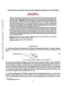
of which we want to inspect the 13-th approximant using the approximate option. This approximant is computed symbolically and afterwards evaluated at z = 6.5 using Maple’s built-in decimal arithmetic. For the latter we choose the decimal precision t = 46. The particular choice N = 13 and t = 46 allows an easy comparison with the results from Section 4. At this moment we do not want to emphasize the role of the continued fraction tail. For this option we select none. The output screen lists 46 digits of the approximant value, as well as the absolute and relative error, where the exact value of erfc(6.5) is replaced by a very high precision estimate (computed at a multiple of the chosen precision t). Apparently the 13-th approximant yields 27 significant digits at z = 6.5. Special functions : cont i nue d f ra ct i on a nd s e ri e s re pre s e nt a t i ons

Function categories

Handbook

Software

A. Cuyt W. B. Jones V. Petersen B. Verdonk H. Waadeland

F. Backeljauw S. Becuwe M. Colman A. Cuyt T. Docx

Error function and related integrals » erfc » approximate

Elementary functions Gamma function and related functions Error function and related integrals erf dawson erfc Fresnel C Fresnel S

Representation

Input

Exponential integrals and related functions

rhs

J-fraction

Hypergeometric functions

parameters

none

Confluent hypergeometric functions

base

10

digits

46

approximant

13

z

6.5

Bessel functions

tail estimate

(5 ≤ digits ≤ 999) (1 ≤ approximant ≤ 999)

none

standard

improved

user defined (simregular form)

Continue

© C opyright 2 0 0 8 Universiteit A nt werpen

c ontac t@ c fhblive.ua.ac .be

Figure 2

Special functions : 10

cont i nue d f ra ct i on a nd s e ri e s re pre s e nt a t i ons

Function categories

Handbook

Software



Error function and related integrals » erfc » approximate

Elementary functions Gamma function and related functions Error function and related integrals erf dawson erfc Fresnel C Fresnel S

Representation

Input

Exponential integrals and related functions

rhs

J-fraction

Hypergeometric functions

parameters

none

Confluent hypergeometric functions

base

10

digits

46

approximant

13

z

6.5

Bessel functions

(5 ≤ digits ≤ 999) (1 ≤ approximant ≤ 999)

none

tail estimate

standard

improved

user defined (simregular form)

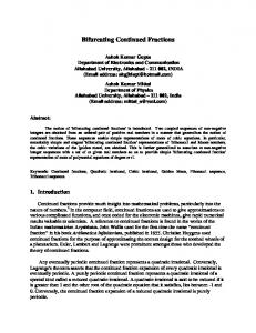
Output approximant

3.842148327120647469875804525852808522764701220e-20

absolute error

1.792e-46

relative error

4.663e-27

tail estimate

0

Continue

© C opyright 2 0 0 8 Universit eit A nt werpen


Figure 3 Information about the domain of convergence of a series or continued fraction is obtained from the constraints argument, which is used for instance in the construction of (6). In the web interface we distinguish between violating a parameter constraint and the case where the variable is taken outside the domain of convergence. In the latter, a result is still returned with the warning that it may be unreliable. This aproach allows the user to observe the behaviour of the representation outside its domain. In the former, when a parameter constraint is violated, no value is returned. When a user suspects the discovery of a new continued fraction representation, its equivalence with the existing continued fractions supported in the Maple library can be checked using the equivalent function. The function checks if the sequences of approximants are the same. Since we are dealing with limit-periodic continued fractions, this comes down to comparing all approximants up to the least common multiple of the numbers of general elements increased with the maximum number of begin elements. This can only be done in the Maple programming environment, not via the webpage. In Maple the library can also be searched for the predefined continued fractions and series using the query command. Predefined formulas can be retrieved using the formula command. 4. Evaluating the special functions reliably. In the wake of the continued fraction handbook, again making use of series and continued fraction representations, a numeric software library for the provably correct evaluation

11

of a large family of special functions is being developed as well. For the time being use of this library is restricted to the real line. So in the sequel we denote the function variable by x rather than by z. We only summarize the workings here and refer to [2] for more detailed information. The library will be made available on the handbook’s website and will be accessible via the web interface under the option evaluate. Let us assume to have at our disposal a scalable precision IEEE 754-854 compliant [9] floating-point implementation of the basic operations, comparisons, base and type conversions, in the rounding modes upward, downward, truncation and round-to-nearest. Such an implementation is characterized by four parameters: the internal base β, the precision t and the exponent range [L, U ]. We target implementations in β = 2 at precisions t ≥ 53, and implementations for use with β = 2i or β = 10i where i > 1. We denote by ⊕, , ⊗, the exactly rounded (to the nearest) floating-point implementation of the basic operations +, −, ×, ÷ in the chosen base β and precision t. Hence these basic operations are carried out with a relative error of at most 1/2 β −t+1 which is also called 1/2 ulp in precision t: (x ~ y) − (x ∗ y) 1 −t+1 ≤ β , ∗ ∈ {+, −, ×, ÷}. 2 x∗y In the other three rounding modes the upper bound on the relative error doubles to 1 ulp. The realization of an implementation of a function f (x) in that floating-point environment is essentially a three-step procedure: 1) For a given argument x, the evaluation f (x) is often reduced to the evaluation of f for another argument x ˜ lying within specified bounds and for which there exists an easy relationship between f (x) and f (˜ x). The issue of argument reduction is a topic in its own right and mostly applies to only the simplest transcendental functions [12]. In the sequel we skip the issue of argument reduction and assume for simplicity that x = x ˜. 2) After determining the argument, a mathematical model F for f is constructed, in our case either a partial sum of a series or an approximant of a continued fraction, and a truncation error |f (x) − F (x)| (9) |f (x)| comes into play, which needs to be bounded. In the sequel we systematically denote the approximation F (x) ≈ f (x) by a capital italic letter. 3) When implemented, in other words evaluated as F(x) by replacing each mathematical operation ∗ by its implementation ~, this mathematical model is also subject to a round-off error |F (x) − F(x)| (10) |f (x)| which needs to be controlled. We systematically denote the implementation F(x) of F (x) in capital typewriter font. The technique to provide a mathematical model F (x) of a function f (x) differs substantially when going from a fixed finite precision context to a finite scalable precision

12

context. In the former, the aim is to provide an optimal mathematical model, often a so-called best approximant, satisfying the truncation error bound imposed by the fixed finite precision and requiring as few operations as possible. In the latter, the goal is to provide a generic technique, from which a mathematical model yielding the imposed accuracy, is deduced at runtime. Hence best approximants are not an option since these models have to be recomputed every time the precision is altered and a function evaluation is requested. At the same time the generic technique should generate an approximant of as low complexity as possible. We also want our implementation to be reliable, meaning that a sharp interval enclosure for the requested function evaluation is returned without any additional cost. If the total error |f (x) − F(x)|/|f (x)| is bounded by αβ −t+1 , then a reliable interval enclosure for the function value f (x) is [F(x) − αβ e+1−t+1 , F(x) + αβ e+1−t+1 ],

blogβ |f |c = e.

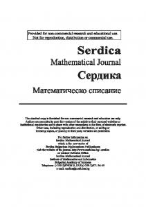
To make sure that the total error |f (x) − F(x)|/|f (x)| is bounded by αβ −t+1 we must determine N such that for the mathematical model F (x), being either a partial sum of degree N or an N -th approximant of a continued fraction, the truncation error f (x) − F (x) α −t+1 ≤ β f (x) 2 and evaluate F (x), in a suitable working precision s larger than the user precision t, such that the computed value F(x) satisfies F (x) − F(x) α −t+1 ≤ β . f (x) 2 How this can be guaranteed for series and continued fraction models is described in [2], where it is also illustrated with some examples. We content ourselves here with a teaser of the web interface to the evaluate option in the Figures 4 and 5. In its verbose mode the web interface also returns the computed N (obtained from the tolerated truncation error), the working precision s (obtained from the tolerated round-off error), the tail estimate wN (if applicable) and the at runtime computed theoretical truncation and round-off error bounds. We choose to evaluate the complementary error function at x = 6.5 and request the total relative error (truncation and round-off acccumulated, taking into account any 2 √ errors in the computation of the factor e−x / π as well) to be bounded above by one decimal unit (β = 10) in the 40-th digit (not counting any leading zeroes). In other words we expect to receive a computed value ERFC(6.5) that satisfies erfc(6.5) − ERFC(6.5) ≤ 10−39 erfc(6.5) In the option evaluate the base is not restricted to 10. It can be set to 10i (1 ≤ i ≤ 7) or 2i (1 ≤ i ≤ 24). We have made the choice β = 10 here in order to compare the

13

output to the one from Figure 3. The program returns the requested 40 digits with the information (verbose mode) that N = 13, s = 46, tN ≈ −0.037. Needless to say that the effortless but appropriate choice of the tail tN has greatly improved the accuracy of the result, from 27 to 40 significant digits!

Special functions : cont i nue d f ra ct i on a nd s e ri e s re pre s e nt a t i ons

Function categories

Handbook

Software



Error function and related integrals » erfc » evaluate

Elementary functions Gamma function and related functions

Representation

Error function and related integrals erf dawson erfc Fresnel C Fresnel S Exponential integrals and related functions Hypergeometric functions Confluent hypergeometric functions Bessel functions

Input parameters

none

base

10^k

digits

40

verbose x

yes

k= 1

(base 2^k: 1 ≤ k ≤ 24; base 10^k: 1 ≤ k ≤ 7)

(5 ≤ digits ≤ 999) no

6.5

Continue

© C opyright 2 0 0 8 Universiteit A ntwerpen


Figure 4

Special functions : 14

cont i nue d f ra ct i on a nd s e ri e s re pre s e nt a t i ons

Function categories

Handbook

Software



Error function and related integrals » erfc » evaluate

Elementary functions Gamma function and related functions

Representation

Error function and related integrals erf dawson erfc Fresnel C Fresnel S Exponential integrals and related functions Hypergeometric functions Confluent hypergeometric functions Bessel functions

Input parameters

none

base

10^k

digits

40

verbose

yes

x

k= 1

(base 2^k: 1 ≤ k ≤ 24; base 10^k: 1 ≤ k ≤ 7)

(5 ≤ digits ≤ 999) no

6.5

Output value

3.842148327120647469875804543768776621449e-20

absolute error bound

3.520e-61

relative error bound

9.162e-42

tail estimate

-3.691114343068676e-02

working precision

46

approximant

13

Continue

© C opyright 2 0 0 8 Universiteit A ntwerpen

Figure 5


5. Future work. The project is an ongoing project and future work includes the inventory and symbolic implementation of representations for the Coulomb wave functions, the Legendre functions, the Riemann zeta function and other frequently used special functions. As they become available, the list of functions available in the tabulate (Section 2) and approximate (Section 3) options on the web is enlarged. As far as the option evaluate (Section 4) is concerned, an interface to this numeric library from within Maple and from Matlab is under development, and a similar implementation in the complex plane is the subject of future research. As the work evolves, the webpage www.cfhblive.ua.ac.be will be updated. References [1] M. Abramowitz and I.A. Stegun. Handbook of mathematical functions with formulas, graphs and mathematical tables. U.S. Government Printing Office, NBS, Washington, D. C., 1964. [2] F. Backeljauw, S. Becuwe, and A. Cuyt. Validated evaluation of special mathematical functions. Lecture Notes in Artificial Intelligence, 5144:206–216, 2008.

15

[3] F. Backeljauw and A. Cuyt. A continued fraction package for special functions. ACM Transactions on Mathematical Software, 2008. Submitted. [4] Barry A. Cipra. A new testament for special functions? SIAM News, 31(2), 1998. [5] A. Cuyt, V. Brevik Petersen, B. Verdonk, H. Waadeland, and W. B. Jones. Handbook of Continued Fractions for Special Functions. Springer, 2008. [6] A. Erdélyi, W. Magnus, F. Oberhettinger, and F.G. Tricomi. Higher transcendental functions, volume 1. McGraw-Hill, New York, 1953. [7] A. Erdélyi, W. Magnus, F. Oberhettinger, and F.G. Tricomi. Higher transcendental functions, volume 2. McGraw-Hill, New York, 1953. [8] A. Erdélyi, W. Magnus, F. Oberhettinger, and F.G. Tricomi. Higher transcendental functions, volume 3. McGraw-Hill, New York, 1955. [9] Floating-Point Working Group. IEEE standard for binary floating-point arithmetic. SIGPLAN, 22:9–25, 1987. [10] D. Lozier. NIST Digital Library of Mathematical Functions. Annals of Mathematics and Artificial Intelligence, 38(1–3), May 2003. [11] Cleve Moler. The tetragamma function and numerical craftmanship. MATLAB News & Notes, 2002. [12] J.-M. Muller. Elementary functions: Algorithms and implementation. Birkhäuser, 1997.