Continuous and Discrete-Time Optimal Controls for an Isolated
Recommend Documents
and Mechanics, ANAS, Baku, Azerbaijan. Abstract. In this paper, we continue investigation of the problem considered in our earlier works. The paper deals with ...
Jul 20, 1995 - ... in part by the National Science Foundation under grants IRI-9222926, IRI- ... library information systems, entertainment industry, educational.
Jul 20, 1995 - of a structured presentation is hiccup{free when it satis es the temporal constraints imposed on the display of each object. \Reboot" Ber94] is an ...
namics of this model, characterize the optimal controls related to drug therapy, ... Key words and phrases: Optimal controls, Mycobacterium tuberculosis, ...
Oct 5, 2014 - we construct a series of finite element spaces Vh1 , Vh2 , ··· , Vhn defined ... of multilevel meshes Thk (k = 1, 2, ··· ,n) such that VH â Vh1 â Vh2 ...
Dec 18, 2018 - The means of handling the irregular real wind farm ... After an upstream wind turbine extracts kinetic energy from wind, .... farm layout optimization problem with more advanced optimization .... Two-Dimensional Analytical Wake Model .
Michael Herty. Technische ... CLAUS KIRCHNER, MICHAEL HERTY, SIMONE GÃTTLICH AND AXEL KLAR approach has ...... [5] C. D'Apice, R. Manzo. A fluid ...
Apr 8, 2018 - 1âKey Laboratory for Applied Statistics of MOE, School of ... Bergquist (2007), discontinuous processes, i.e., processes where parts or batches are ... a complete overview on the subject of the theory of opetimal design ... on the bra
Feb 9, 2011 - The proposed algorithms are built upon the linear minimum variance unbiased estimation. Unlike the other existing approaches such as those.
Ziyu Guo. May 2016. 1 Introduction to Optimal Control. Optimal control theory aims to solve optimization problems. It is an exten- sion of the classical calculus of ...
MATHEMATICAL PROGRAMMING METHODS ... This paper deals with suitable stochastic optimization in continuous casting process of steel via ..... Rao, S. S. Engineering Optimization Theory and Practice, Fourth Edition, New Jersey, Willey ...
Abstract. In this paper we study continuous-time Markov decision processes with the average sample-path reward (ASPR) criterion and possibly unbounded ...
results on a microgrid test system verify the effectiveness and superiority of the presented .... times, limited EV range and high battery replacement cost [12], which, to a certain .... PDF used to depict the probabilistic nature of solar irradiance
Feb 8, 2013 - criteria) between the payoff of the option and the terminal value of the hedging ... price of the option is related to two components: first, the ...
Without a centralized database to draw fromâa ... need to pull data from its own databases (as well as from ... for Pe
The Department of Health and Human Services of United States of America cited 4 ...... E.E.M. Monninkhof, P.P.D.L.P.M. van der Valk, G.G.A. Zielhuis, E.H. Walters, ... C. Turro, M. Taha, âQoE assesment of MPEG-DASH in polimedia eLearning.
special cases of optimal low-thrust orbit-transfer problems, but the general continuous-thrust problem requires full numerical integration of each initial condition ...
Methods- From August 2011 through September 2012, 71 patients ... 2 MATERIALS AND METHODS .... from operation theatre to ICU on ventilatory support.
L. Jetto*,â and V. Orsini. Dipartimento di Ingegneria dell'Informazione, UniversitÑ Politecnica delle Marche, Ancona, Italy. SUMMARY. This paper presents a new ...
tion is derived in Section III using a dynamic programming type argument. We present ... Optimal control over an RF channel with limited controls. Limited control ...
with the hip joint center ï¬xed and the foot rigidly attached to the pedal. The model ... local minimum before the maximum number of function calls. number of data ...
Apr 27, 2012 - DOI: 10.1002/oca.2023. Further results on H1 control for discrete-time uncertain singular systems with interval time-varying delays in state and ...
Dec 15, 2010 - [4] P. Caldiroli, R. Musina, On a variational degenerate elliptic problem, Nonlinear Diff. Equa. Appl., 7(2000), 187â199. [5] V. Chiad`o Piat, ...
Continuous and Discrete-Time Optimal Controls for an Isolated
Jul 19, 2017 - ed the continuous-time model by including the maximum queue lengths .... control problem (see (6)) with free terminal time . The decision variable ... ple (PMP) to derive the optimal solution to the continuous- time model ...
Hindawi Journal of Sensors Volume 2017, Article ID 6290248, 11 pages https://doi.org/10.1155/2017/6290248
Research Article Continuous and Discrete-Time Optimal Controls for an Isolated Signalized Intersection Jiyuan Tan,1 Xiangyun Shi,1 Zhiheng Li,2 Kaidi Yang,3 Na Xie,4 Haiyang Yu,5 Li Wang,1 and Zhengxi Li1 1
Beijing Key Lab of Urban Intelligent Traffic Control Technology, North China University of Technology, Beijing 100144, China Graduate School at Shenzhen, Tsinghua University, Shenzhen 518055, China 3 The Institute for Transport Planning and Systems (IVT), ETH Zurich, Zurich, Switzerland 4 School of Management Science and Engineering, Central University of Finance and Economics, Beijing 100081, China 5 Beijing Key Laboratory for Cooperative Vehicle Infrastructure Systems and Safety Control, School of Transportation Science and Engineering, Beihang University, Beijing 100191, China 2
1. Introduction Along with the fast increase of auto population, urban streets are becoming more crowded nowadays. To relieve congestions and reduce accidents, various traffic control methods have been proposed since the late 1950s [1]. As a typical traffic scenario, oversaturated intersections attracted consistent interest during the last six decades [2, 3]. The term “oversaturated” means the following: the vehicles that remained since the last cycle plus the vehicles that newly arrived exceed the capacity of the intersection. This leads to the carryover of vehicle queues (at least in one leg of the intersection) to the next cycle. Discussions on the road networks that consist of many oversaturated intersections can be found in researches done by Chang and Sun [4], Di Febbraro and Sacco [5], Dotoli and Fanti [6], Ma [7, 8], and Sun et al. [9, 10]. In the research done by Varaiya [11] and Le et al. [12], the study of pressure-based signal control developed stability properties of a decentralized signal timing policy for networks with stochastic arrivals.
But for a real-time signal timing optimization problem, the data that could be used is the arriving information of vehicles in the recent several signal cycles (data could be gotten by connecting vehicle technology, etc.). The optimization objects and scenarios are different between the model in this paper and pressure-based policies. This paper will focus on the isolated oversaturated intersection. Usually, researchers aim to find an optimal signal timing plan that minimizes the total delay of vehicles passing this intersection. The total delay is often defined as the time integral of the sum of all queue lengths for all legs of the intersection over a given time horizon. However, the total delay is a nonlinear and nonconvex function of control variables (e.g., green phases), which makes it difficult to optimize. One promising approach is to apply heuristic algorithms to solve the formulated optimization problem. For example, the genetic algorithm was applied by Park et al. [13] to optimize the total delay. An alternative approach is to first approximate the nonconvex total delay with some convex functions and then solve the newly formulated optimization problem. The
2 rest of this paper will focus on the second approach within a typical traffic scenario: an isolated intersection with only two movements. There are mainly two kinds of convexified models for this scenario. The first kind of models originated from Gazis [3] who used continuous-time differential equations to describe the traffic dynamics. The cycle length, departing flow rates, and arriving flow rates in Gazis [3] were all assumed to be constant. Michalopoulos and Stephanopoulos [14, 15] extended the continuous-time model by including the maximum queue lengths constraints and time-variant arrival flow rates. Such formulations led to a classical control problem that can be solved via the Pontryagin Maximum Principle (PMP) [16]. However, the obtained continuous-time signal timing plan should be discretized into the corresponding discrete-time signal timing plan that can be executed in practice. The second kind of models uses discrete-time difference equations to describe the traffic dynamics [7, 8, 17–19]. The corresponding design problem can then be formulated as a linear programming (LP) problem [20–25]. One interesting question that naturally arises is how to depict the difference and connection between the discrete-time model and the continuous-time model. Recently, Ioslovich et al. [26] studied the formulated LP problem by considering the corresponding continuous-time approximation model and gave an elegant approximate solution in continuous-time forms. However, it was not verified how this approximate solution differs from the accurate solution (the solution obtained by the continuous-time model). Whether a discretized version of this continuous-time approximate solution is still optimal to the LP problem also needs further discussions. Zou et al. [27] have given a preliminary result on the relationship between the continuous-time model and the discrete-time model. Zou et al. applied a graphical method to adjust the continuous-time approximate solution to a discrete-time accurate solution. They assumed that both streams are dispatched simultaneously and the adjustment method does not influence the clearance cycle. It is shown that the approximate solution can be adjusted to the optimal solution by changing the green ratio in the switching cycle. However, the discrete-time LP problem in Ioslovich et al. [26] is more complex than the one considered in [27], since the two streams are allowed to be cleared at different times. Merely changing the green ratios at the switching cycle may not obtain the accurate solution. In this paper, the LP problems proposed by Ioslovich et al. [26] are directly attacked using the strong duality theorem [28]. It is first shown that the approximate solution and the accurate solution do not coincide in many situations. Then, the relationship between the approximate solution and the accurate solution will be discussed. The errors introduced by discretization are carefully studied. It is shown that, in many cases, the discretized approximate solution can be converted to the accurate solution within a few gradient descent adjustments. Finally, an algorithm is proposed to implement this conversion. These findings shed light on the connection between the continuous-time and discrete-time signal timing models.
Journal of Sensors
m1
m2
Figure 1: An isolated intersection with two one-way movements 𝑚1 and 𝑚2 .
To give a detailed analysis, the rest of this paper is arranged as follows. Section 2 introduces the LP problem proposed by Ioslovich et al. [26] and lists the nomenclature used in this paper. Section 3 proposes two counterexamples to show that the optimality of the discretized approximate solution may not hold. Section 4 discusses the difference and connection between the discrete-time model and the continuoustime model. Finally, Section 5 concludes the paper.
2. Problem Presentation 2.1. Nomenclature and Assumptions. For presentation simplicity, the nomenclature in this paper follows Ioslovich et al. [26] as shown in Nomenclature List. Similar to Ioslovich et al. [26], consider an isolated intersection with two one-way streams 𝑚1 and 𝑚2 governed by signal lights, as shown in Figure 1. Note that the two-stream isolated intersection is chosen as an initial building block to understand the connection between the continuous-time model and the discretetime model. This is a widely applied treatment even in recent works (e.g., [23]). Nevertheless, this assumption can be relaxed to consider general intersections. Both the continuous model and the discrete model are able to handle cases with more generalized intersections. Although it is hard to directly compare the two types of models in generalized intersections, we expect that the findings in this paper can shed light on more generalized intersections. Likewise, the following assumptions are imposed as in Ioslovich et al. [26]. Assumption 1. (a) Each signal cycle starts with a green light for 𝑚1 . (b) There is no lost time for each cycle. Suppose that the green ratio for stream 𝑚1 in cycle 𝑘 is denoted as 𝑢(𝑘); the green ratio for stream 𝑚2 is then equal to 1 − 𝑢(𝑘).
Journal of Sensors
3
(c) The arrival flow rates and the saturation departure flow rates of both streams are constant over time. Denote 𝑎𝑖 as the arrival flow rates for 𝑚𝑖 and 𝑑𝑖 as the departure flow rates. (d) Without loss of generality, 𝑚1 is assumed to be the main stream (i.e., 𝑑1 > 𝑑2 ). (e) For some reasons (e.g., physical constraints), both streams are constrained by minimum green ratios. Define 𝑢min and 1 − 𝑢max as the minimum green ratios for 𝑚1 and 𝑚2 , respectively; then, the constraint on 𝑢(𝑘) is represented as 𝑢min ≤ 𝑢(𝑘) ≤ 𝑢max . (f) There exists a signal timing strategy such that queues in both streams can be cleared finally but may not be in the
min s.t.
𝑁
𝐽𝐷 = ∑ [𝑞1 (𝑘) + 𝑞2 (𝑘)] + 𝑘=0
same cycle. Define 𝑢𝐿 = 𝑎1 /𝑑1 and 𝑢𝐻 = 1 − 𝑎2 /𝑑2 . This assumption is written as 𝑢𝐿 < 𝑢𝐻, 𝑢𝐿 < 𝑢max , and 𝑢min < 𝑢𝐻. (g) Cycle lengths are known to be constant 𝑇. In Assumption 1, (a)–(f) are inherited from Ioslovich et al. [26] directly and (g) is added to simplify the discussion. In fact, if cycle lengths are not fixed, a similar conclusion can still be drawn but the detailed timing plan is much more complicated. 2.2. The Discrete-Time LP Model and Its PMP Solution. Similar to Ioslovich et al. [26], the discrete-time model is formulated as the following problem to minimize the total delay of vehicles: 𝑎1 + 𝑎2 𝑁−1 𝑇 ∑ 𝑢 (𝑘) 2 𝑘=0
for 𝑘 = 0, 1, . . . , 𝑁 − 1. In (1)–(5), the objective function is a linear approximation for total delay. The decision variables are 𝑢(𝑘), 𝑘 = 0, 1, . . . , 𝑁. For presentation convenience, it is assumed that the number of total cycles 𝑁 is large enough such that both streams are cleared before cycle 𝑁. Equations (2) and (3) represent the evolution of both queues in time. Equation (4) gives the upper and lower bound of the green ratio in each cycle. Equation (5) is the initial queue lengths. It is easy to verify that this LP problem is equivalent to the Relaxed Discrete-Event MaxPlus Problem proposed by Haddad et al. [22]. In Ioslovich et al. [26], the above LP (see (1)–(5)) was transformed into an equivalent continuous-time optimal control problem (see (6)) with free terminal time𝑡𝑓 . The decision variable is V(𝑡).
𝑞𝑖 (𝑡𝑓 ) = 0, 𝑖 = 1, 2. (6) Ioslovich et al. [26] applied Pontryagin Maximum Principle (PMP) to derive the optimal solution to the continuoustime model (see (6)). Particularly, the following four cases were discussed with respect to the order of 𝑢𝐿 , 𝑢𝐻, 𝑢min , and 𝑢max : (I) 𝑢𝐿 < 𝑢min < 𝑢𝐻 < 𝑢max ; (II) 𝑢𝐿 < 𝑢min < 𝑢max < 𝑢𝐻; (III) 𝑢min < 𝑢𝐿 < 𝑢max < 𝑢𝐻; (IV) 𝑢min < 𝑢𝐿 < 𝑢𝐻 < 𝑢max . Table 1 lists the solution. The optimal continuous-time solution is denoted asV∗ (𝑡). 𝑡𝑠 is the switching time where the optimal control switches. 𝑀 and 𝑅 are represented as
For example, Figure 2 illustrates the evolution of queue lengths under the optimal solution for Case I(a). It is observed that the optimal solution is a two-stage strategy, namely, bang-bang control. The green ratio remains 𝑢max at first, causing the length of stream 𝑚1 to decrease sharply and stream 𝑚2 to increase. After the switching time 𝑡𝑠 , the green ratio changes into 𝑢min and both streams start to decrease. The optimal switch-over point where the solution switches from maximum to minimum green split is given in Table 1.
4
Journal of Sensors Table 1: The optimal solution to the continuous model.
Case
Condition
Solution
I(a)
𝑞1,int >𝑅 𝑞2,int
{ {𝑢max , V∗ (𝑡) = { { {𝑢min ,
𝑞1,int 𝑀 𝑞2,int
V∗ (𝑡) = 𝑢max
III(b)
𝑞1,int 𝑡𝑠 {𝑢𝐿 ,
𝑞1,int 𝑑1 (𝑢max − 𝑢𝐿 )
{ {𝑢max , 𝑡 < 𝑡𝑠 V∗ (𝑡) = { { 𝑡 > 𝑡𝑠 {𝑢𝐿 ,
𝑞1,int 𝑑1 (𝑢max − 𝑢𝐿 )
V∗ (𝑡) = 𝑢min
IV
The discretized solution of V∗ (𝑡) is obtained as follows. Suppose the cycle length is 𝑇; the discretization is done as 𝑘 = 0, 1, . . . , 𝑁 − 1.
(8)
(t)
𝑢𝐷 (𝑘) = V∗ (𝑘𝑇) ,
uG;R uGCH
For presentation simplicity, the solution 𝑢𝐷(𝑘), 𝑘 = 0, 1, . . . , 𝑁 − 1, is called the discretized approximate solution in the rest of this paper.
2.3. The Steady State and the Steady-State Solution. According to Haddad et al. [22], the steady state is defined as the state where the queue lengths are the same in the beginning and end of each cycle. This means, given the green ratio for a certain stream, the queue lengths of this stream keep the same in a certain period. Denote the queue lengths in the steady state as 𝑞𝑖,ss , 𝑖 = 1, 2, and the green ratio in the steady state as 𝑢ss . So, considering a single-cycle version of discrete-time model (see (1)–(5)), the steady state can be formulated into the following model:
0
ts
t
tf
Figure 2: An illustration of the queue lengths and optimal timing plan in Case I(a).
The objective equation (9) is a linear approximation of delay in a single cycle. Equations (10) and (11) depict the queue evolution. Equation (12) gives the bound of the green ratio.
Journal of Sensors
5
The optimal green ratio 𝑢ss is called the steady-state solution. Haddad et al. [22] gave a neat analytical form of 𝑢ss as follows: {max {𝑢𝐿 , 𝑢min } , 𝑎1 < 𝑎2 , 𝑢ss = { min {𝑢𝐻, 𝑢max } , 𝑎1 > 𝑎2 . {
(13)
According to Haddad et al. [22], the two streams that follow the discrete-time model (see (1)–(5)) will eventually enter the steady state under Assumptions (a)–(g). Therefore, in the accurate solution, the green ratios in the steady state are the steady-state solution 𝑢ss .
3. The Nonoptimality of the Discretized Approximate Solution In this section, it is shown that the discretized approximate solution does not always coincide with the accurate solution. The term “coincide” here means that the discretized approximate solution is not always optimal for the discrete-time model. In particular, two counterexamples are constructed. The first counterexample is used to deal with Case I and Case II where the minimum green ratio 𝑢min plays an important role in the approximate solution. In contrast, the second counterexample is used to handle Case III and Case IV where the minimum green ratio 𝑢min does not influence the approximate solution. The two counterexamples are as follows. Counter Example 1 (for Case I and Case II). The parameters are set as 𝑞1,int = 60, 𝑞2,int = 20, 𝑑1 = 0.55, 𝑑2 = 0.30, 𝑎1 = 0.15, 𝑎1 = 0.10, 𝑢min = 0.40, 𝑢max = 0.80, 𝑇 = 160, and 𝑁 = 6. Then, the accurate solution and the discretized approximate solution are shown in Figure 3(a). Counter Example 2 (for Case III and Case IV). The parameters are set as 𝑞1,int = 40, 𝑞2,int = 40, 𝑑1 = 0.60, 𝑑2 = 0.35, 𝑎1 = 0.15, 𝑎1 = 0.10, 𝑢min = 0.15, 𝑢max = 0.80, 𝑇 = 100, and 𝑁 = 25. Then, the accurate solution and the discretized approximate solution are shown in Figure 3(b). As is shown in Figure 3, the accurate solution deviates from the discretized approximate solution in two ways. In Counterexample 1, the accurate solution roughly remains as a bang-bang form before the system enters steady state. The difference concentrates around the switching cycle and steady state. However, in Counterexample 2, the accurate solution exhibits oscillation and differs from the discretized approximation solution in almost every cycle. Such deviations are caused by discretization and can be classified into two categories. The first category of deviations is caused by the discretization of the model constraints. For the continuous-time model, the queue length for stream 𝑚𝑖 is lower-bounded by the constraint 𝑞1 (𝑘) ≥ 0, while for the discrete-time model, the corresponding constraint is 𝑞1 (𝑘) ≥ 𝑎1 𝑇(1 − 𝑢(𝑘)). When cycle length 𝑇 is large, the discretization of model constraints may introduce huge errors. In Counterexample 1, the switching time locates in the middle of a cycle. As
shown in Figure 4, the discretization leads to waste of green ratio around the switching cycle due to the restriction of the minimum green ratio. When 𝑇 is small enough, the solution of the continuous-time model and the solution of the discrete-time model are coherent. A proper 𝑇 should be selected to ensure consistency. The second category deviation is caused by the discretization of the approximate solution. In Counterexample 2, the clearance time of stream 𝑚1 locates in the middle of a cycle. So, the discretization causes oscillation in the accurate solution.
4. The Relationship between the Discretized Approximate Solution and the Accurate Solution In this section, the connection between the discrete approximate solution and the accurate solution is further discussed. For Case I and Case II, the errors are relatively concentrated. The discretized approximate solution does not deviate largely from the accurate solution in many cases. In fact, the discretized approximate solution can be modified to the accurate solution by some minor adjustments; see Algorithm 1. The details of adjustments will be discussed in Sections 4.1–4.3. For Case III and Case IV, however, the dispersed errors make it hard to adjust the solution in a few steps. However, for some carefully chosen cycle length, the accurate solution coincides with the discretized approximate solution. For example, in Case III, if the cycle length is chosen as 𝑇 = 𝑞1,int /[𝑛𝑑1 (𝑢max −𝑢𝐿 )+(𝑑1 −𝑎1 )𝑢𝐿 ], where 𝑛 is any positive integer, the accurate solution can be written as {𝑢max , 𝑘 ≤ 𝑛, (14) 𝑢 (𝑘) = { 𝑢 , 𝑘 > 𝑛. { 𝐿 It is easy to show that this accurate solution coincides with the corresponding discretized approximate solution. In the rest of this section, the discussion will focus on the adjustments for Case I, and the adjustments for Case II are similar. For presentation simplicity, define several denotations before starting the discussion. Define ̂𝑘1 and ̂𝑘2 , respectively, as the clearance cycle indices in which streams 𝑚1 and 𝑚2 are cleared exactly: ̂𝑘 fl max {𝑘 : 𝑞 (𝑘) > 𝑎 𝑇 (1 − 𝑢 (𝑘))} , 1 1 1
(15)
̂𝑘 fl max {𝑘 : 𝑞 (𝑘) > 0} . 2 2
(16)
Apparently, in Case I(a), it holds that ̂𝑘1 ≤ ̂𝑘2 . So, both streams enter steady state after cycle ̂𝑘2 . Note that there is also a switch in the discretized approximate solution. Define ̂𝑘𝑠 as the switching cycle index where switch occurs; that is, ̂𝑘 : min {𝑘 : 𝑢 (𝑘) < 𝑢 } . 𝑠 max
(17)
The adjustments contain two parts. Section 4.1 deals with the adjustment in the steady state. Section 4.2 includes
6
Journal of Sensors
0.7
0.8
0.6
0.7
0.5
0.6
u(k)
u(k)
0.8
0.4
0.5 0.4
0.3
0.3 0
1
2
3
4
5
6
0
1
2
3
4
5
k
k (a)
(b)
Figure 3: The two counterexamples. The dotted line represents the discretized approximate solution. The solid line represents the accurate solution.
Figure 4: An illustration of the error caused by discretization. The dotted line represents the queue lengths in the continuous-time model. The solid line represents the queue lengths in the discretetime model.
the adjustment around the switching cycle. Both parts are summarized as Algorithm 1. The optimality of Algorithm 1 will be proven in the Appendix. Finally, Counterexample 1 in Section 3 is revisited to better illustrate the adjustments. 4.1. The Steady-State Adjustment. The adjustment for the steady state is shown in lines (34)–(38) in Algorithm 1. Since the steady-state solution is optimal for the discrete-time model after the two streams enter steady state, 𝑢(𝑘) can be set as 𝑢 (𝑘) = 𝑢ss , 𝑘 > ̂𝑘2 .
(18)
However, in the clearance cycle ̂𝑘2 , the optimal green ratio is not 𝑢ss due to discretization. So, 𝑢(̂𝑘2 ) can be set as follows:
(19)
4.2. The Adjustment around the Switch. The adjustment around the switching cycle is shown in lines (2)–(33) in Algorithm 1. There are two cases of adjustment: increasing the green ratios after the switch and decreasing the green ratios before the switch. For presentation simplicity, this subsection only handles the case of increasing the green ratios after the switch. The adjustment to the other case is similar except for some details; see Algorithm 1, lines (9)–(20). This adjustment can be viewed as a gradient descent approach to gradually reduce the total delay. It operates in three steps: (1) determine the direction of adjustment; (2) update the green ratio; (3) check feasibility of the new green ratio. It will be proven in the Appendix that such adjustment operations can be finished in a few steps. Due to constraint equations (3) and (4), the discrete-time model is a nonsmooth model. Thus, a subdifferential will be used instead of a gradient. Without loss of generality, assume that both streams are cleared after the switching cycle (i.e., ̂𝑘 ≥ ̂𝑘 ). The case of ̂𝑘 < ̂𝑘 can be transformed easily to the 1 𝑠 1 𝑠 case of ̂𝑘1 > ̂𝑘𝑠 (Algorithm 1, lines (2)–(8)). In the first step, the direction of adjustment is determined by calculating the subdifferential. Denote the subdifferential of the total delay 𝐽𝐷 with respect to 𝑢(̂𝑘𝑠 ) as 𝜕𝐽𝐷. Define the function 𝑄(̂𝑘1 , ̂𝑘2 , ̂𝑘𝑠 ) as 𝑄 (̂𝑘1 , ̂𝑘2 , ̂𝑘𝑠 ) 𝑎 + 𝑎2 {[𝑑2 (̂𝑘2 − ̂𝑘𝑠 ) − 𝑑1 (̂𝑘1 − ̂𝑘𝑠 ) + 1 ] 𝑇, 𝑎1 < 𝑎2 , (20) 2 ={ ̂ ̂ ̂ ̂ 𝑎1 > 𝑎2 , {[𝑑2 (𝑘2 − 𝑘𝑠 ) − 𝑑1 (𝑘1 − 𝑘𝑠 ) + 𝑎1 ] 𝑇,
so as to represent the subdifferential in a more convenient way. Clearly, the case of increasing the green ratios after the switch corresponds to the condition of 𝑄(̂𝑘1 , ̂𝑘2 , ̂𝑘𝑠 ) < 0.
Journal of Sensors
7 (1) Set 𝑢(𝑘) as the discretized approximate solution. Calculate ̂𝑘1 , ̂𝑘2 , ̂𝑘𝑠 by Eq. (15)-(16); (2) if ̂𝑘1 < ̂𝑘2 then (3) Set 𝑢(̂𝑘𝑠 − 1) ← min{(𝑞1 (̂𝑘𝑠 − 1)/𝑇)/(𝑑1 − 𝑎1 ), 𝑢max } and set 𝑢(𝑘) ← 𝑢min , 𝑘 ≥ ̂𝑘𝑠 ; (4) Update ̂𝑘2 by Eq. (16) and set ̂𝑘1 ← ̂𝑘𝑠 ; (5) if 𝑢(̂𝑘𝑠 − 1) ≤ 𝑢min then (6) 𝑢(̂𝑘𝑠 − 1) ← 𝑢min , ̂𝑘𝑠 ← ̂𝑘1 − 1 and update ̂𝑘1 and ̂𝑘2 by Eq. (15) and (16); (7) end (8) end (9) while 𝑄(̂𝑘1 , ̂𝑘2 , ̂𝑘𝑠 − 1) > 0 do; ̂𝑘 ← ̂𝑘 − 1. Update 𝑢(̂𝑘 − 1) such that stream 𝑚 is cleared exactly in cycle ̂𝑘 ; (10) 2 2 𝑠 2 2 (11) Update ̂𝑘1 by Eq. (15); (12) if 𝑄(̂𝑘1 , ̂𝑘2 + 1, ̂𝑘𝑠 − 1) < 0 then ̂𝑘 ← ̂𝑘 +1. Find the minimum ̂𝑘 such that 𝑄(̂𝑘 + 1, ̂𝑘 , ̂𝑘 − 1) < 0; (13) 2 2 1 1 2 𝑠 (14) Update 𝑢(̂𝑘𝑠 − 1) such that stream 𝑚1 is cleared exactly in cycle ̂𝑘1 ; (15) Set ̂𝑘1 ← ̂𝑘1 + 1; (16) end (17) if 𝑢(̂𝑘𝑠 − 1) < 𝑢min then (18) 𝑢(̂𝑘𝑠 − 1) ← 𝑢min , ̂𝑘𝑠 ← ̂𝑘𝑠 − 1 and update ̂𝑘1 and ̂𝑘2 by Eq. (15) and (16); (19) end (20) end (21) while 𝑄(̂𝑘1 , ̂𝑘2 , ̂𝑘𝑠 ) < 0 do ̂𝑘 ← ̂𝑘 + 1. Update 𝑢(̂𝑘 ) such that stream 𝑚 is cleared exactly in cycle ̂𝑘 ; (22) 2 2 𝑠 2 2 (23) Update ̂𝑘1 by Eq. (15); (24) if 𝑄(̂𝑘1 , ̂𝑘2 , ̂𝑘𝑠 ) > 0 then ̂𝑘 ← ̂𝑘 − 1. Find the maximum ̂𝑘 such that 𝑄(̂𝑘 , ̂𝑘 , ̂𝑘 ) ≥ 0; (25) 2 2 1 1 2 𝑠 (26) Update 𝑢(̂𝑘𝑠 ) such that stream 𝑚1 is cleared exactly in cycle ̂𝑘1 ; (27) else if 𝑄(̂𝑘1 , ̂𝑘2 + 1, ̂𝑘𝑠 ) > 0 and 𝑢(̂𝑘𝑠 ) ≤ 𝑢max then (28) break; (29) end (30) if 𝑢(̂𝑘𝑠 ) > 𝑢max then (31) 𝑢(̂𝑘𝑠 ) ← 𝑢max , ̂𝑘𝑠 ← ̂𝑘𝑠 + 1 and update ̂𝑘1 and ̂𝑘2 by Eq. (15)-(16); (32) end (33) end (34) if 𝑎1 > 𝑎2 and 𝑢max > 𝑢𝐻 then (35) Calculate 𝑞1 (𝑘), 𝑞2 (𝑘), by Eq. (2)-Eq. (3); (36) Set 𝑢(̂𝑘2 ) ← 𝑢𝐻 − 𝑞2 (̂𝑘2 )/(𝑑2 𝑇); (37) for 𝑘 ∈ (̂𝑘2 , 𝑁) do 𝑢(𝑘) = 𝑢𝐻 ; (38) end Algorithm 1: The adjusting algorithm for the discretized approximate solution in Case I(a).
There are three situations based on the queue evolution in clearance cycles ̂𝑘1 and ̂𝑘2 . (1) Stream 𝑚1 is cleared exactly in cycle ̂𝑘1 ; that is, 𝑞(̂𝑘1 + 1) = 𝑎1 𝑇(1 − 𝑢(̂𝑘1 )) = 𝑞1 (̂𝑘1 ) − 𝑑1 𝑇(𝑢(̂𝑘1 ) − 𝑢𝐿 ). The subdifferential in this situation is calculated as 𝜕𝐽𝐷 = [𝑄 (̂𝑘1 + 1, ̂𝑘2 , ̂𝑘𝑠 ) , 𝑄 (̂𝑘1 , ̂𝑘2 , ̂𝑘𝑠 )] ,
(21)
where “[𝑎, 𝑏]” means the closed interval between real numbers 𝑎 and 𝑏. The physical meaning of the subdifferential 𝐽𝐷 is shown as follows. The total delay changes if a slight disturbance is imposed on 𝑢(̂𝑘𝑠 ). Denote Δ𝑢(̂𝑘𝑠 ) as the increment in 𝑢(̂𝑘𝑠 )
and Δ𝐽𝐷 as the corresponding change in total delay. If Δ𝑢(̂𝑘𝑠 ) > 0, then Δ𝐽𝐷 can be calculated as Δ𝐽𝐷 = (𝑑2 (̂𝑘2 − ̂𝑘𝑠 ) − 𝑑1 (̂𝑘1 − ̂𝑘𝑠 ) +
𝑎1 + 𝑎2 ) 𝑇Δ𝑢 (̂𝑘𝑠 ) (22) 2
= 𝑄 (̂𝑘1 , ̂𝑘2 , ̂𝑘𝑠 ) Δ𝑢 (̂𝑘𝑠 ) . Similarly, if Δ𝑢(̂𝑘𝑠 ) < 0, the corresponding changes in total delay are written as Δ𝐽𝐷 = 𝑄(̂𝑘1 + 1, ̂𝑘2 , ̂𝑘𝑠 )Δ𝑢(̂𝑘𝑠 ). Therefore, if 𝑄(̂𝑘1 , ̂𝑘2 , ̂𝑘𝑠 ) < 0, the total delay can be reduced by increasing 𝑢(̂𝑘𝑠 ). If 𝑄(̂𝑘1 , ̂𝑘2 , ̂𝑘𝑠 ) ≥ 0 and 𝑄(̂𝑘1 + 1, ̂𝑘2 , ̂𝑘𝑠 ) < 0, neither increasing nor decreasing 𝑢(̂𝑘𝑠 ) will
8
Journal of Sensors
5. Conclusion
u(k)
0.8
0.4
0
1
2
3
4
5
6
This paper studies the continuous-time and discrete-time signal timing models for the classical isolated signalized intersection with only two one-way vehicle flows. Against intuitions, the nonequivalence between the solutions of the two models is first shown by two counterexamples. Then, the differences between the solutions of the two models are explained. Finally, an algorithm is proposed to transform the discretized continuous-time solution to the discrete-time solution for many cases. Via this gradient descent based algorithm, a more concrete link is set up between the continuoustime and discrete-time signal timing models.
k Discretized solution Step 1 Step 2 Step 3
Step 4 Step 5 Optimal solution
Appendix Proof of the Optimality of Algorithm 1 The optimality is stated in the following theorem.
Figure 5: The adjustment of the discretized approximate solution.
Theorem A.1. The solution derived by Algorithm 1 is optimal for Case I(a). render a better total delay and thus the optimal 𝑢(̂𝑘𝑠 ) is achieved. (2) Stream 𝑚2 is cleared exactly in cycle ̂𝑘2 ; that is, 𝑞2 (̂𝑘2 + 1) = 0 = 𝑞2 (̂𝑘2 ) − 𝑑2 𝑇(𝑢𝐻 − 𝑢(̂𝑘2 )). The subdifferential can be calculated similarly as 𝜕𝐽𝐷 = [𝑄(̂𝑘1 , ̂𝑘2 , ̂𝑘𝑠 ), 𝑄(̂𝑘1 , ̂𝑘2 + 1, ̂𝑘𝑠 )]. Then, if 𝑄(̂𝑘1 , ̂𝑘2 +1, ̂𝑘𝑠 ) < 0, the total delay can be reduced by increasing 𝑢(̂𝑘𝑠 ). If 𝑄(̂𝑘1 , ̂𝑘2 + 1, ̂𝑘𝑠 ) ≥ 0 and 𝑄(̂𝑘1 , ̂𝑘2 , ̂𝑘𝑠 ) < 0, the optimal choice of 𝑢(̂𝑘𝑠 ) is obtained. (3) Both streams are not cleared exactly in their clearance cycles. Then, the subdifferential is 𝜕𝐽𝐷 = {𝑄(̂𝑘1 , ̂𝑘2 , ̂𝑘𝑠 )}. If 𝑄(̂𝑘1 , ̂𝑘2 , ̂𝑘𝑠 ) < 0, the total delay can be reduced by increasing 𝑢(̂𝑘𝑠 ). In the second step, the green ratio 𝑢(̂𝑘𝑠 ) is updated by reducing ̂𝑘1 and increasing ̂𝑘2 . The green ratio 𝑢(̂𝑘𝑠 ) is calculated such that either stream 𝑚1 or stream 𝑚2 is cleared exactly in its clearance cycle. The detailed calculation is shown in Algorithm 1 (lines (24)–(29)). The third step is the feasibility check of whether the new green ratio 𝑢(̂𝑘𝑠 ) satisfies the constraint equation (4). In the case of increasing 𝑢(̂𝑘𝑠 ), the only possible violation is 𝑢(̂𝑘𝑠 ) > 𝑢max . Therefore, if the feasibility check fails, 𝑢(̂𝑘𝑠 ) is set as 𝑢max and a new bang-bang solution is obtained. Then, the algorithm goes back to the first step and determines the direction of adjustment.
Theorem A.1 will be proven by the strong duality theorem (shown as Lemma A.2). Lemma A.2 (strong duality theorem for linear programming). A primal feasible solution and a dual feasible solution to a linear programming problem are optimal if and only if the corresponding primal and dual objectives are the same. Proof of Theorem A.1. For presentation simplicity, only the case of increasing the green ratios after the switch will be considered in this proof. The other case can be similarly proven. Since the adjustment for the switching cycle (lines (21)–(33)) is a gradient descent approach and the discrete LP model is apparently feasible, the algorithm will eventually terminate. The dual problem to the discrete LP model (see (1)–(5)) is written as 𝐽̃𝐷 = max
2
∑𝑞𝑖,int 𝛼 (0) 𝑖=1
𝑁−1
+ ∑ min {𝑆 (𝑘) 𝑢max , (𝑘) 𝑢min }
(A.1)
𝐾=0
𝑁−1
+ ∑ [𝑑1 𝑢𝐿 𝛼1 (𝑘) − 𝑑2 𝑢𝐻𝛼2 (𝑘)] 4.3. The Numerical Examples. In this subsection, Counterexample 1 in Section 3 is revisited to illustrate the steps of Algorithm 1. Recall that the parameters are 𝑑1 = 0.55, 𝑑2 = 0.3, 𝑎1 = 0.15, 𝑎2 = 0.10, 𝑢min = 0.4, 𝑢max = 0.8, 𝑞1,int = 60, 𝑞1,int = 20, 𝑇 = 160, and 𝑁 = 6. Algorithm 1 will be applied to adjust the discretized approximate solution. The detailed operation is shown in Table 2. The adjustment of the discretized approximate solution is also shown in Figure 5.
There are three situations when the iteration of lines (21)–(33) terminates. (1) The iteration terminates at line (28). Then, 𝑢(̂𝑘𝑠 ) is given such that stream 𝑚2 is cleared exactly. The corresponding ̂𝑘1 , ̂𝑘2 , and ̂𝑘𝑠 satisfy 𝑄(̂𝑘1 , ̂𝑘2 , ̂𝑘𝑠 ) ≤ 0 and 𝑄(̂𝑘1 , ̂𝑘2 + 1, ̂𝑘𝑠 ) > 0. (2) The iteration terminates at line (21) and 𝑢(̂𝑘𝑠 ) is set as 𝑢max . The corresponding ̂𝑘1 , ̂𝑘2 , and ̂𝑘𝑠 satisfy 𝑄(̂𝑘1 , ̂𝑘 , ̂𝑘 ) ≥ 0. 2
Substituting (A.5) and (A.6) into (A.4), 𝑆(𝑘) can be represented as
𝑎1 + 𝑎2 , 2
𝑘 < ̂𝑘1 , ̂𝑘 ≤ 𝑘 ≤ ̂𝑘 , 1 2
(A.7)
𝑘 > ̂𝑘2 .
This proves that the primal and dual objective values are equal. By Lemma A.2, both primal and dual solutions are optimal. Therefore, Algorithm 1 gives the optimal solution for Case I(a).
The proofs of the three situations is similar. Only the first situation is handled here. Moreover, assume 𝑎1 < 𝑎2 . The proof of 𝑎1 > 𝑎2 is the opposite. Denote 𝜖1 and 𝜖2 , respectively, as 𝜖1 = 0 and 𝜖2 = −𝑄(̂𝑘1 , ̂𝑘2 , ̂𝑘𝑠 )/𝑑2 . Then the dual solution is rewritten as
𝑠
(3) The iteration terminates at line (21) and 𝑢(̂𝑘𝑠 ) is given such that stream 𝑚1 is cleared exactly. The corresponding ̂𝑘1 , ̂𝑘2 , and ̂𝑘𝑠 satisfy 𝑄(̂𝑘1 , ̂𝑘2 , ̂𝑘𝑠 ) ≥ 0 and 𝑄(̂𝑘1 + 1, ̂𝑘2 , ̂𝑘𝑠 ) < 0.
Known Constants 𝑁: The total number of cycles in the observation period 𝑇: The cycle length of the isolated intersection 𝑚𝑖 : The two streams, 𝑖 = 1, 2 𝑎𝑖 : The arrival rate of stream 𝑚𝑖 , 𝑖 = 1, 2 𝑑𝑖 : The saturation departure flow rate of stream 𝑚𝑖 , 𝑖 = 1, 2
10 𝑞𝑖,int :
The initial queue length of stream 𝑚𝑖 , 𝑖 = 1, 2 The green ratio that keeps stream 𝑚1 𝑢𝐿 : unchanged (i.e., 𝑢𝐿 fl 𝑎1 /𝑑1 𝑢𝐻: The green ratio that keeps stream 𝑚2 unchanged (i.e., 𝑢𝐻 fl (𝑑2 − 𝑎2 )/𝑑2 𝑢min , 𝑢max : The minimum and maximum bounds of green ratio The steady-state solution of the 𝑢ss : discrete-time model. Variables and Functions regarding the Continuous-Time Model 𝑡𝑠 :
The switching time of signal timing plan in the continuous-time optimal solution The final time in the 𝑡𝑓 : continuous-time model 𝐽𝐶: The objective of the continuous-time model, representing the approximate total delay V(𝑡): The green time ratio of stream 𝑚𝑖 at time 𝑡, the decision variable for continuous-time model V∗ (𝑡): The approximate solution, that is, the optimal solution to the continuous-time model. Variables and Functions regarding the Discrete-Time Model 𝑢(𝑘): The green time ratio of stream 𝑚𝑖 in cycle 𝑘, the decision variable for the discrete-time model 𝑞𝑖 (𝑘): The queue lengths of stream 𝑚𝑖 in the beginning of cycle 𝑘, 𝑘 = 0, . . . , 𝑁 − 1 ̂𝑘 : The index of the cycle in which the stream 1 𝑚1 is cleared ̂𝑘 : The index of the cycle in which the stream 2 𝑚2 is cleared ̂𝑘 : The index of the cycle in which 𝑢(𝑘) 𝑠 switches from 𝑢max to 𝑢min 𝐽𝐷: The objective of the discrete-time model, representing approximate total delay 𝑢∗ (𝑘): The accurate solution, that is, the optimal solution to the discrete-time model 𝑢𝐷(𝑘): The discretized solution of V∗ (𝑡).
Conflicts of Interest The authors declare that they have no conflicts of interest.
Acknowledgments Support by Beijing Natural Science Foundation (4164083), National Natural Science Foundation of China (61603005, 71303269), Fundamental Research Funds for the Central Universities, and Central University of Finance and Economics
Journal of Sensors Major Research Task of Fostering Project (14ZZD006) is gratefully acknowledged.
References [1] F. Webster, Traffic signal settings. Road Research Technical Paper 39. Great Britain Road Research Laboratory, London, UK, 1958. [2] D. Green, “Control of oversaturated intersections,” Operational Research Quarterly, vol. 18, no. 2, pp. 161–173, 1967. [3] D. C. Gazis, “Optimum control of a system of oversaturated intersections,” Operations Research, vol. 12, no. 6, pp. 815–831, 1964. [4] T.-H. Chang and G.-Y. Sun, “Modeling and optimization of an oversaturated signalized network,” Transportation Research Part B: Methodological, vol. 38, no. 8, pp. 687–707, 2004. [5] A. Di Febbraro and N. Sacco, “On modelling urban transportation networks via hybrid Petri nets,” Control Engineering Practice, vol. 12, no. 10, pp. 1225–1239, 2004. [6] M. Dotoli and M. P. Fanti, “An urban traffic network model via coloured timed Petri nets,” Control Engineering Practice, vol. 14, no. 10, pp. 1213–1229, 2006. [7] X. Ma, H. Yu, Y. Wang, Y. Wang, and J. Gomez-Gardenes, “Large-scale transportation network congestion evolution prediction using deep learning theory,” PLoS ONE, vol. 10, no. 3, Article ID e0119044, 2015. [8] X. Ma, Z. Tao, Y. Wang, H. Yu, and Y. Wang, “Long shortterm memory neural network for traffic speed prediction using remote microwave sensor data,” Transportation Research Part C: Emerging Technologies, vol. 54, pp. 187–197, 2015. [9] W. Sun, Y. Wang, G. Yu, and H. X. Liu, “Quasi-optimal feedback control for a system of oversaturated intersections,” Transportation Research Part C: Emerging Technologies, vol. 57, pp. 224–240, 2015. [10] W. Sun, Y. Wang, G. Yu, and H. X. Liu, “Quasi-optimal feedback control for an isolated intersection under oversaturation,” Transportation Research Part C: Emerging Technologies, vol. 67, pp. 109–130, 2016. [11] P. Varaiya, “Max pressure control of a network of signalized intersections,” Transportation Research Part C: Emerging Technologies, vol. 36, pp. 177–195, 2013. [12] T. Le, P. Kov´acs, N. Walton, H. L. Vu, L. L. H. Andrew, and S. S. P. Hoogendoorn, “Decentralized signal control for urban road networks,” Transportation Research Part C: Emerging Technologies, vol. 58, pp. 431–450, 2015. [13] B. Park, C. J. Messer, and T. Urbanik II, “Traffic signal optimization program for oversaturated conditions: genetic algorithm approach,” Transportation Research Record, no. 1683, pp. 133– 142, 1999. [14] P. G. Michalopoulos and G. Stephanopoulos, “Oversaturated signal systems with queue length constraints—I: single intersection,” Transportation Research, vol. 11, no. 6, pp. 413–421, 1977. [15] P. G. Michalopoulos and G. Stephanopoulos, “Oversaturated signal systems with queue length constraints-II. Systems of intersections,” Transportation Research, vol. 11, no. 6, pp. 423– 428, 1977. [16] L. Pontryagin, V. Boltyanskii, R. Gamkrelidze, and E. Mishchenko, The mathematical theory of Optimal processes, vol. 43, Wiley-Interscience, 1962. [17] R. Allsop, “SIGSET: A computer program for calculating traffic signal settings,” Transportation Engineering Control, vol. 13, no. 2, pp. 58–60, 1971.
Journal of Sensors [18] R. E. Allsop, “Estimating the traffic capacity of a signalized road junction,” Transportation Research, vol. 6, no. 3, pp. 245–255, 1972. [19] R. E. Allsop, “SIGCAP: A computer program for assessing the traffic capacity of signal-controlled road junctions,” Transportation Engineering Control, vol. 17, no. 819, pp. 338–341, 1976. [20] J. Haddad, B. De Schutter, D. Mahalel, and P.-O. Gutman, “Steady-state and N-stages control for isolated controlled intersections,” in Proceedings of the 2009 American Control Conference, ACC 2009, pp. 2843–2848, June 2009. [21] J. Haddad, B. De Schutter, D. Mahalel, I. Ioslovich, and P.O. Gutman, “Optimal steady-state traffic control for isolated intersections,” in Proceedings of the 6th IFAC symposium on robust control design, 2009, pp. 96–101. [22] J. Haddad, B. De Schutter, D. Mahalel, I. Ioslovich, and P.O. Gutman, “Optimal steady-state control for isolated traffic intersections,” Institute of Electrical and Electronics Engineers. Transactions on Automatic Control, vol. 55, no. 11, pp. 2612–2617, 2010. [23] L. Li, K. Yang, Z. Li, and Z. Zhang, “The optimality condition of the multiple-cycle smoothed curve signal timing model,” Transportation Research Part C: Emerging Technologies, vol. 27, pp. 46–57, 2013. [24] K. Han, V. V. Gayah, B. Piccoli, T. L. Friesz, and T. Yao, “On the continuum approximation of the on-and-off signal control on dynamic traffic networks,” Transportation Research Part B: Methodological, vol. 61, pp. 73–97, 2014. [25] F. Zhu and S. V. Ukkusuri, “A linear programming formulation for autonomous intersection control within a dynamic traffic assignment and connected vehicle environment,” Transportation Research Part C: Emerging Technologies, vol. 55, pp. 363– 378, 2015. [26] I. Ioslovich, J. Haddad, P.-O. Gutman, and D. Mahalel, “Optimal traffic control synthesis for an isolated intersection,” Control Engineering Practice, vol. 19, no. 8, pp. 900–911, 2011. [27] B. Zou, J. Hu, and Y. Zhang, “The optimal discretized timing plan for individual oversaturated intersections,” in Proceedings of the 2012 15th International IEEE Conference on Intelligent Transportation Systems, ITSC 2012, pp. 1656–1660, September 2012. [28] D. G. Luenberger and Y. Ye, Linear and Nonlinear Programming, vol. 116 of International Series in Operations Research & Management Science, Springer, New York, NY, USA, 3rd edition, 2008.