Continuous Distance Computation for Planar Non-holonomic Motions with Constant Accelerations Enrique J. Bernabeu
Abstract—A method for computing the distance between two mobile objects following linear or arc-like motions with constant accelerations is introduced in this paper. This distance is obtained without stepping or discretizing any object’s motion. Objects are modeled by bi-dimensional convex hulls. The distance-computation algorithm obtains the instant in time when two mobile objects are at their minimum translational distance of separation or penetration. The distance and the instant in time are parallely computed. This method is so fast that can be run as frequent as new information from the world is received.
D
I. INTRODUCTION
ETECTING a collision in motion planning is still an open research line in Robotics. Nowadays, powerful motion planners are developed, where collision tests are an unavoidable step and represent, in general, a decisive timeconsuming part in the planning algorithms. A recent example and with important social impact is shown by [1], [2]. An estimated motion for an obstacle and a desired one for the robotized car Boss are stepped at a determined time instants. Then, collision tests between the positions of both objects at each considered time instant are run. Objects are modeled by boxes or circles. This collisiondetection technique has several limitations as shown by [3]. Nevertheless, this approach is frequent in the literature in order to detect collisions between mobile objects [4]. Other group of collision-detection methods is called Continuous Collision Detection (CCD). In general, these methods also provide, if objects collide, the instant in time of the first contact. Some representative examples are [3], [5−7]. In any case, with all these types of methodologies is really a hard problem to find the exact instant in time when two mobile objects are at their minimum distance. This paper introduces a technique for obtaining the instant in time when two objects are at their minimum translational distance. If objects do not collide, then the Euclidean distance is computed, otherwise, their minimum translation distance of penetration, defined as [8], is returned. Objects are modeled by convex hull geometries and follow planar non-holonomic motions with constant accelerations. Specifically, only linear and arc-like motions are considered in this paper. Considering the previous author’s work in [9] as a collision detector, the main contributions of this paper are Manuscript received September 15, 2009. Enrique J. Bernabeu is with Instituto Universitario de Automática e Informática Industrial, Universidad Politécnica de Valencia, Camino de Vera s/n, Valencia, E-46022, Spain (e-mail:
[email protected]).
twofold: arc-like motions are also considered, and obstacles follow motions with non-null acceleration. The method in this paper is fast enough to be run as frequent as new information from the world is received. And, it is intended to be used as a collision-detection module in sampling-based algorithms for vehicle-like robots. II. MINKOWSKI DIFFERENCE OF TWO MOTIONS In this Section, two mobile objects with null accelerations and linear motions are being considered. Objects are modeled by either a polytope [10] or a spherical-extended polytope (s-tope) [11]. Motions and objects are constrained to be bi-dimensional. Formally, an s-tope is the convex hull of a finite set of spheres, circles if bi-dimensional, S={s0,s1,…,sn−1} with si=(ci,ri), where ci is the center and ri is the radius. S-tope SS contains an infinite set of swept spheres/circles expressed by
{
S S = s =(c, r ): c = c0 +∑i =1 λ i (ci −c0 ), r = r0 +∑i =1 λ i (ri − r0 ), n −1
n −1
}(1)
si = (ci , ri )∈ S , λ i ∈ [0,1], ∑i =1 λ i ≤ 1 n −1
Note that, if all radii ri are zero, then (1) is the polytope definition [10]. Consequently, a polytope is a particular case of an s-tope. For this reason, from now, all the objects in this paper are generally modeled by s-topes. The order of the stope SS is the number of spheres/circles in S. Let SA(ts) be the A‘s position at the instant in time ts. A is modeled by an n-order s-tope with SA(ts)={s0A(ts),s1A(ts),…, sn−1A(ts)}, where ciA(ts)∈ℜ2 are the centers and riA∈ℜ are the radii of circles siA(ts)=(ciA(ts),riA), i=0,1,…,n−1. As A’s size does not change, then radii riA do not depend on time. A’s speed at ts is stated by the vector vA(ts)∈ℜ2. ||vA(ts)|| indicates the magnitude and vA(ts) the direction. Let SB(ts) be the position of a mobile object B at ts. B is modeled by an m-order s-tope, with SB(ts)={s0B(ts),s1B(ts),…, sm−1B(ts)}. cjB(ts)∈ℜ2 and rjB∈ℜ are the centers and radii of circles sjB(ts), with j=0,1,…,m−1. B’s speed at ts is vB(ts)∈ℜ2. ||vB(ts)|| indicates the magnitude and vB(ts) the direction. Each of the infinite intermediate positions of mobile objects A and B from ts to a given time horizon Δt, i.e. SA(t) and SB(t) for all t∈[ts,ts+Δt], are parameterized by λ∈[0,1] as S A (t ) ={siA (t ) = (ciA (t ), ri A ) : ciA (t ) = ciA (t s ) + λ ⋅Δt ⋅v A (t s ) ; i = 0,.., n −1} S B (t ) ={s jB (t ) = (c jB (t ), rjB ): c jB (t ) = c jB (t s ) + λ⋅Δt ⋅v B (t s ) ; j= 0,.., m −1} ∀t : t = t s + λ⋅Δt ; t∈[t s ,t s + Δt ] and λ∈[0,1]
(2)
s3A(ts)
s2A(ts)
A at t1
A at t2
A at t3
distance at the instant in time when A and B are at their minimum translational distance (MTD) of separation or penetration. Fig. 3 also shows dOM computation. Formally, dOM is
A at ts+Δt
A at ts
A
s1 (ts)
s0A(ts)
B at t2
s0B(ts)
B at ts+Δt
d OM = min s1B(ts)
B at t3
B at t1
B at ts Fig. 1. Two stepped motions. SA(ts)={s0A(ts),s1A(ts),s2A(ts),s3A(ts)} with riA=0, ∀i, and SB(ts)={s0B(ts),s1B(ts)} represent A and B positions at ts. Dashed lines show the distance between A and B at the instants in time ts,t1,t2,t3,ts+Δt.
An example for two objects following a linear motion with constant speed is shown in fig. 1. Distances at each different instant in time are also shown. These distances have been obtained by applying the algorithm in [12], which is an update from the GJK one in [10]. Then, they have been obtained by computing the separation from the origin point O to the Minkowski difference between s-topes A and B at each considered instant in time. Formally, the Minkowski difference between A and B at a given t, is an s-tope SA−B(t), defined by the set of n×m circles {sijA−B(t)} {sijA −B (t )}={(cijA −B (t ), rijA −B ) : cijA −B (t ) = ciA (t ) − c jB (t ); rijA −B = ri A + ri B ; ∀i, j}
{
{sijM (t )}= (cijM (t ), rijM ) : rijM = ri A + ri B ;
[
][
]
}
cijM (t ) = ciA (t s ) + λ⋅Δt ⋅v A (t s ) − c jB (t s ) + λ ⋅Δt ⋅v B (t s ) ; ∀i, j
(4)
∀t : t = t s + λΔt ; t∈ [t s , t s + Δt ] and λ∈[0,1]
Note that, for instance, if λ=0, then SM(t) represents the Minkowski difference between A and B at ts, i.e., SA−B(ts). And if λ=1, then SM(t) states the Minkowski difference of A and B at ts+Δt, i.e, SA−B(ts+Δt). Each sijM(t) for all t∈[ts,ts+Δt] sweeps an area consisting of a rectangle whose ends are capped off with circles. This geometrical figure is referred to as stadium by [13]. Then, SM(t) is formed by n×m stadiums, and each one is defined by three parameters: a start point cijM(ts)=ciA(ts)−cjB(ts), a radius rijM=riA+rjB and a linear axis pM(λ)∈ℜ2. pM(λ) is parametrically defined by λ∈[0,1] as p M (λ) = λ ⋅Δt ⋅(v A (t s ) − v B (t s ) )
(5)
The stadium’s axis is the locus swept by cijM(t) from ts to ts+Δt. All the axes of the stadiums are equal and their length is ||pM(1)||. Fig. 3 shows SM(t) with its n×m stadiums. Note that SM(t) contains all the Minkowski differences in fig. 2. Proposition 1: The distance from O to SM(t), dOM, is the
A
B
τ ∈ℜ 2
If A and B do not collide during their respective motions, then dOM is the Euclidean distance. Nevertheless, if they collide, then the sign of dOM is negative and dOM acquires the meaning of the MTD of penetration given by [8]. Proof: It is trivial and is a direct consequence of the SM(t) definition given by (4) and from conclusions by [10] Let cabM(ts)=caA(ts)−cbB(ts), rabM with axis pM(λ) be the stadium in SM(t) that is the closest to O, then the distance between O and SM(t) is from (4)
[
][
]
d OM = caA (t s ) + λ⋅Δt ⋅v A (t s ) − c bB (t s ) + λ⋅Δt ⋅v B (t s ) − rabM (7)
dOM is obtained by finding λm, with λm∈[0,1] that minimizes (7). Given that the axes of the stadiums in SM(t) are linear, λm is obtained by computing Oc, with Oc=cijM(ts)+pM(λm), i.e. by projecting O onto such an axis. Therefore,
(
(3)
Fig. 2 shows all the Minkowski difference s-topes between A and B positions at all the time instants from fig. 1. The Minkowski difference between A and B positions for all t∈[ts,ts+Δt] is called SM(t) and is defined by the set of n×m circles {sijM(t)}. sijM(t) are parameterized by λ∈[0,1] as
{ inf {|| τ ||: dist (S (t )+ τ, S (t)) = 0}} (6)
t∈[ t s , t s + Δt ]
)
λ m = − (caA (t s ) − c bA (t s ))⋅ p M (1) || p M (1)|| 2
(8)
Then dOM=||Oc||−rabM. As parameter λ is related with time, the time instant tOM, when MTD between A and B is dOM, is t OM = t s + λ m ⋅Δt ; where t OM ∈ [t s , t s + Δt ] and λ m∈ [0,1] (9)
Substituting λm in (2), SA(tOM) and SB(tOM) are obtained. They respectively represent the positions of mobile objects A and B at time tOM, i.e., when their MTD is dOM. Nevertheless, distance computation in (7) fails when O is inside the area delimited by the axes of the stadiums. As SM(t) is a Minkowski difference, then A and B will collide during their motions. When this situation is presented, dOM has to be reformulated as finding λm∈[0,1] that maximizes d OM = −
( [c (t )+ λ⋅Δt ⋅v (t )]−[c (t ) + λ⋅Δt ⋅v (t )] + r ) (10) A a
s
A
s
B b
s
B
s
M ab
where caA(ts)−cbB(ts), rabM states the axis of the external stadium in SM(t) that is the closest to O. In this situation, note that radius rabM is added. Sign of dOM is negative, because it holds a translational distance of penetration. λm and tOM are respectively computed as indicated by (8), and (9). An open problem is finding the closest stadium in SM(t) to O. This problem is solved by using a GJK-based algorithm, specifically by defining the appropriate support and solution functions. This point will be explained in the next sections. As a conclusion of this Section, the instant in time, tOM, when two mobile objects are at their MTD, while they are following linear paths with constant speeds, is fast obtained without stepping any of the objects motions.
s31A−B(ts)
s21A−B(ts) S
s30A−B(ts)
A−B
(ts)
SA−B(t1) SA−B(t2) SA−B(t3)
s11A−B(ts) s10 s20
A− B
(ts)
A− B
s00A−B(ts)
(ts)
SA−B(ts+Δt)
s01A−B(ts) O
Fig. 2. Minkowski differences s-topes between A and B positions at the instants ts, t1, t2, t3, ts+Δt (from fig. 1) and their distances to origin point O c31M(ts) c M(t ) c M(t ) 21
30
s
s
SA−B(t1)
SA−B(ts)
SA−B(t2) SA−B(t3)
M
c11 (ts)
SA−B(ts+Δt) c10M(ts)
c20M(ts)
c01M(ts)
c00M(ts) External edges
d OM
O
Fig. 3. Stadiums in SM(t) (black) from motions in fig. 1. For clarity, only the axes (dashed lines) and the extreme circles of the stadiums are depicted. c10M(ts), c31M(ts) are the start point of the external stadiums. Their external edges are also shown. Dotted lines show the Minkowski difference s-topes from fig. 2.
III. DISTANCE BETWEEN TWO OBJECTS FOLLOWING LINEAR MOTIONS WITH CONSTANT ACCELERATION A technique for determining, without stepping, the instant in time when two mobile objects are at their MTD, while they are following linear motions with constant accelerations, is introduced in this Section. Let A be a mobile object, modeled by an n-order s-tope, whose position at ts is SA(ts)={s0A(ts),s1A(ts),…,sn−1A(ts)}, where ciA(ts)∈ℜ2 and riA∈ℜ are respectively the centers and radii of circles siA(ts)=(ciA(ts),riA), ∀i. A’s speed at ts is vA(ts)∈ℜ2. Its constant acceleration is aA∈ℜ. Let B be a mobile object, modeled by an m-order s-tope, whose position at ts is SB(ts)={s0B(ts),s1B(ts),…,sm−1B(ts)}. cjB(ts)∈ℜ2 and rjB∈ℜ are respectively the centers and radii of circles sjB(ts), ∀j. B’s speed at ts is vB(ts)∈ℜ2 and its constant acceleration is aB∈ℜ. Assuming a time horizon Δt, positions SA(t)={(ciA(t),riA), ∀i}, SB(t)={cjB(t),rjB), ∀j} for all t∈[ts,ts+Δt] are parameterized by λ∈[0,1], as follows ciA (t ) = ciA (t s ) + λ⋅Δt ⋅v A (t s ) + 0.5⋅λ 2⋅Δt 2⋅a A⋅vˆ A (t s ); i = 0,.., n −1 c jB (t ) = c jB (t s ) + λ⋅Δt ⋅v B (t s ) + 0.5⋅λ 2⋅Δt 2⋅a B ⋅vˆ B (t s ); j= 0,.., m −1
(11)
where vˆ A (t s ) =v A (t s ) ||v A(t s )|| and vˆB (t s ) =vB (t s ) ||vB (t s )|| . A constraint is introduced in the motions defined by (11). When acceleration is negative, and the time horizon Δt is long enough, the sign of a motion might change, e.g. from moving forward to backwards. Then, if this situation happens, A and B motions in (11) will be conveniently divided. Only motions without changes in their signs are considered. As mentioned in the previous section, the Minkowski dif-
ference between A and B positions for all t∈[ts,ts+Δt] is SM(t) and is defined by n×m stadiums. These stadiums are peculiar because their axes are parabolic. Despite this fact, these geometrical figures are also termed stadiums. Each stadium is defined by a start point ciA(ts)−cjB(ts), a radius riA+rjB, and a parabolic axis pM(λ)∈ℜ2. Axis pM(λ) is common for all the stadiums and is parametrically defined by λ∈[0,1] as p M (λ ) =λ⋅Δt (v A (t s ) − v B (t s ) )+ 0.5⋅λ 2⋅Δt 2 (a A⋅vˆ A (t s ) − a B ⋅vˆ B (t s ) ) (12)
The instant in time tOM, when mobile object A and B are at their MTD, is tOM=ts+λm·Δt, where λm is obtained by finding the parameter that minimizes the distance between O and the external stadium in SM(t) that is the closest to O. A double problem is now presented: a) computing the distance between O and a stadium with a parabolic axis, b) finding the closest external stadium to O. Both problems are solved by applying a GJK-based algorithm, termed LL-GJK. Set Vk in the LL-GJK algorithm always contains one or two stadiums from SM(t). Vk only stores the start point and radius. The subdistance_algorithm computes the distance between O and the stadiums in Vk. Let caA(ts)−cbB(ts), raA+rbB with (caA(ts),raA)∈SA(ts) and (cbB(ts),rbB)∈SB(ts) be a stadium in Vk. The distance between O and such a stadium is determined by finding the solution λc that verifies
d ||caA (t s ) −cbB (t s ) + p M (λ)|| d λ = 0
(13)
||caA(ts)−cbB(ts)+pM(λ)|| only contains one minimum for all λ∈[0,1]. λc is found by applying the root-finding technique, termed Secant method [14], to (13). Experimentally, λ0=0.45 and λ1=0.55 have been confirmed as good choices. Accuracy for the Secant method has been set to 10-6.
LLin-GJK algorithm
LL-GJK algorithm A
B
M
Input: SA(ts), SB(ts), ts, Δt, pM(λ), a one-element set Vin Output: (λm, dOM’)
Input: S (ts), S (ts), ts, Δt, p (λ) Output: (λm, tOM, dOM) or (failure, Vk) 1: k=0, Vk={c0A(ts)−c0B(ts),r0A+r0B} with (c0A(ts),r0A)∈SA(ts) and (c0B(ts),r0B)∈SB(ts) 2: do 3: (λc,dO,Oc,V'k,O_in) ← subdistance_algorithm(Vk) 4: if O_in then return(failure,Vk) 5: compute hM(−Oc), sM(−Oc), h'M(−Oc,λc), s'M(−Oc,λc) 6: if gM(−Oc,λc)=0 then exit_loop endif 7: if s'M(−Oc,λc)=sM(−Oc) or hM(−Oc)>h'M(−Oc,λc) then Vk+1=V'k∪{sM(−Oc)} else Vk+1=V'k∪{s'M(−Oc,λc)} endif 8: k=k+1 9: while true 10: λm=λc; tOM=ts+λm·Δt; dOM=dO−(rpA+rqB) where V'k={cpA(ts)−cqB(ts),rpA+rqB}; with (cpA(ts),rpA)∈SA(ts), (cqB(ts),rqB)∈SB(ts) 11: return(λm, tOM, dOM) After finding λc, Oc and dO are obtained as Oc =caA (t s ) − cbB (t s ) + p M (λ c ); Oc∈ℜ 2 ;
d O =||Oc || ;
(14)
If Vk contains one stadium, then λc, dO, Oc∈ℜ2, V'k=Vk and O_in=false are returned by the subdistance_algorithm. If Vk contains two stadiums, first step consists of checking if O is inside the area delimited by the axes of the stadiums in Vk. If so, O_in=true is returned by the subdistance_algorithm, and then LL-GJK algorithm finishes returning failure (see step 4). On the contrary, if O is not inside, the distance from O to each stadium in Vk is computed. Parameters λc, dO, Oc from the closest stadium to O are returned. V'k only contains the closest stadium. The furthest stadium is rejected and is not considered anymore in the LL-GJK algorithm. In order to find the external stadiums in SM(t), two pairs of support and solution functions are introduced. The first pair of support hM(η) and solution sM(η) functions with η∈ℜ2 is
{
}
hM (η) = max (ciA (t s ) − c jB (t s )) ⋅η+ (ri A + rjB )⋅||η || ∀i, j
with (ciA (t s ), ri A )∈S A (t s ); ( c jB (t s ), rjB )∈S B (t s )
(15)
sM(η) is the circle sM(η)=(caA(ts)−cbB(ts),raA+rbB) that gives value to hM(η), i.e. it represents the stadium in SM(t) whose start point is the furthest from O in the direction η [12], [10]. Given that axes are parabolic, a second pair of support h'M(η,λc) and mapping s'M(η,λc) functions is defined. These functions find the furthest stadium from O in the direction η at the points where the axes of the stadiums are close to O.
{(
)
hM′ (η, λ c ) = max ciA (t s ) −c jB (t s ) + p M (λ c ) ⋅η+ (ri A + rjB )⋅||η || ∀i, j A i
with (c (t s ), ri )∈S (t s ); ( c (t s ), r )∈S (t s ) A
A
B j
B j
B
}
(16)
1: k=0, Vk=Vin 2: do 3: (λc,dO,Oc,V'k,Vk) ← subdistance_in_algorithm(Vk) 4: compute hM(Oc), sM(Oc), h'M(Oc,λc), s'M(Oc,λc) 5: if ĝM(Oc,λc)=0 then exit_loop endif 6: if s'M(Oc,λc)=sM(Oc) or hM(Oc)>h'M(Oc,λc) then Vk+1=V'k∪{sM(Oc)} else Vk+1=V'k∪{s'M(Oc,λc)} endif 7: k=k+1 8: while true 9: λm=λc; dOM’=−(dO+(rpA+rqB)) where V'k={cpA(ts)−cqB(ts),rpA+rqB}; with (cpA(ts),rpA)∈SA(ts), (cqB(ts),rqB)∈SB(ts) 10: return(λm, dOM’) where λc comes from the last execution of the subdistance_ algoritm. The circle s'M(η,λc) represents the stadium in SM(t) that gives value to h'M(η,λc). If sM(η) and s'M(η,λc) represent different stadiums, the one with the greater support function is selected. See step 7 in the LL-GJK algorithm. LL-GJK algorithm finishes when gM(−Oc,λc)=0 is verified with gM(−Oc,λc)=||Oc||2−radius(s'M(−Oc,λc))||Oc||+h'M(−Oc,λc) [12]. In other words, no other stadium is closer to O that the one in Vk, and finally, distance between O and SM(t) is obtained. The distance dOM and time tOM are then returned. Function radius returns the radius of circle s'M(−Oc,λc). If LL-GJK algorithm finishes with a failure, then O is inside the area delimited by the axes of the stadiums and the returned set Vk contains two stadiums. In this case, distances from the inner O to the two external stadiums in SM(t) have to be computed. The LLin-GJK algorithm computes the distance from O to one external stadium. For this reason, LLin-GJK is called twice. Each call receives as input, set Vin, one stadium from the returned Vk. The procedure subdistance_in_algorithm is only different from the subdistance_algorithm in the LL-GJK algorithm when Vk contains two stadiums. In this case, the furthest stadium from O is selected and assigned to V'k, while the other one is rejected and is not used anymore in the current execution of the LLin-GJK algorithm. The external stadium is found in the LLin-GJK algorithm by searching the furthest stadium in the direction Oc. For this reason, h'M(Oc,λc), s'M(Oc,λc), hM(Oc), sM(Oc) are now computed. This makes that the final condition also changes. For this reason, the LLin-GJK algorithm finishes when ĝM(Oc,λc)=−||Oc||2−radius(s'M(Oc,λc))||Oc||+h'M(Oc,λc) is 0. Each execution of the LLin-GJK algorithm returns a parameter λm and a negative distance dOM’. The maximum of the two returned distances holds dOM, i.e. the MTD of penetration between both mobile objects. And, from its associated parameter λm, tOM is then obtained by applying (9).
Two objects, A and B, following linear motions with constant accelerations and the corresponding Minkowski difference SM(t) are shown in fig. 4. The positions, where A and B are at their MTD, are depicted in red. A is modeled by a 4-order s-tope (potytope) and B is a 2-order s-tope. dOM and tOM have been obtained in 6.4 μs in an Intel® CoreTM 2 Duo E8200 processor at 2.66 GHz.
B at ts
B at 1.25s
B at 0.5s
(
)
ciA (t ) = c A +ρ iA cos(θ iA (t )), sin(θ iA (t )) ; i = 0,.., n −1 where
θ (t ) = θ (t s ) + λ⋅Δt ⋅w A (t s ) + 0.5⋅λ 2⋅Δt 2⋅α A A i
A i
(17)
∀t : t = t s + λ⋅Δt ; t∈[t s ,t s + Δt ] and λ∈[0,1]
Let B be an object with a linear motion and modeled by an m-order s-tope. B’s position at ts is SB(ts)={s0B(ts),s1B(ts), …,sm−1B(ts)}. cjB(ts)∈ℜ2 and rjB∈ℜ are respectively the centers and radii of circles sjB(ts), ∀j. B’s speed at ts is vB(ts)∈ℜ2 and its constant acceleration is aB∈ℜ. B’s positions SB(t) for all t∈[ts,ts+Δt] are indicated in (11). Depending on the acceleration and the time horizon, the sign of a motion might change, for instance, from forward to backwards. If this situation happens, A and B motions will be conveniently divided. Only motions without changes in their signs are considered. Each of the n×m stadiums in SM(t) is defined by a start point ciA(ts)−cjB(ts), a radius riA+rjB and an axis. From the definition of the A and B motions in (17) and (11) is concluded that there are n different axes and they are cycloid-like. Each of the n axes piM(λ)∈ℜ2 ∀i is described by λ∈[0,1] as
(
)
piM ( λ ) =ρ iA cos(θ iA (t )), sin(θ iA (t )) − λ⋅Δt ⋅v B (t s ) − − 0.5⋅λ ⋅Δt ⋅a B ⋅vˆ B (t s ); i = 0,.., n −1 2
2
(18)
The angle θiA(t) has been defined in (17). The instant in time when A and B are at their MTD is obtained by applying the algorithms AL-GJK and ALin-GJK. The AL-GJK and ALin-GJK algorithms are respectively analogous to the LL-GJK and LLin-GJK ones. Only the sub
A at 3.5s
B at 2s A at 2s
A at 0.5s
B at 3.5s
A at 1.25s
IV. DISTANCE BETWEEN OBJECTS FOLLOWING LINEAR AND ARC-LIKE MOTIONS WITH CONSTANT ACCELERATIONS The computation of the distance between two mobile objects following respectively linear and arc-like motions with constant accelerations is shown in this Section. Let A be an object with an arc-like motion and modeled by an n-order s-tope. A’s position at ts is SA(ts)={s0A(ts), s1A(ts),…,sn−1A(ts)}, where ciA(ts)∈ℜ2 and riA∈ℜ are the centers and the radii of circles siA(ts)=(ciA(ts),riA), ∀i. A’s arclike motion is centered at cA. With respect to cA, each center ciA(ts) is expressed by a radius ρiA and angle θiA(ts) such that ciA(ts)=cA+ρiA(cos(θiA(ts),sin(θiA(ts)). A’s angular speed at ts is ωA(ts)∈ℜ. A’s constant angular acceleration is αA∈ℜ. Assuming a time horizon Δt, positions SA(t)={(ciA(t),riA), ∀i} for all t∈[ts,ts+Δt] are parameterized by λ∈[0,1] as
A at 2.75s
B at 2.75s
A at ts
External Stadium
(a)
O
d OM External edge Stadium’s axis (b) Fig. 4. Distance between two mobile objects following linear motions, with 2 ||vA(ts)||=2.2 m/s, aA=1 m/s , ||vB(ts)||=3 m/s, aB=−0.5 m/s2, ts=0s, and Δt=5s. (a) A and B positions are only depicted at ts, 0.5s, 1.25s, 2s, 2.75s and 3.5s. The positions where A and B are at their MTD are in red. The MTD of penetration dOM is given at tOM=2.75s. (b) Axes of the eight stadiums in SM(t) and the distance dOM. For clarity, only extreme circles, axis, and edge of the closest external stadium to O are depicted.
tle differences between them are pointed out in this Section. The subdistance_algorithm and subdistance_in_algorithm now compute the distance between O and a cycloid-like axis. Let caA(ts)−cbB(ts), raA+rbB with (caA(ts),raA)∈SA(ts) and (cbB(ts),rbB)∈SB(ts) be a stadium with axis paM(λ). The distance between O and such a stadium is determined by finding the λc that minimizes ||cA−cbB(ts)+paM(λ)||, i.e., by solving d ||c A −cbB (t s ) + paM (λ)|| d λ = 0
(19)
λc is then found by applying the Secant method to (19), but this method works properly if there is one minimum in ||cA−cbB(ts)+paM(λ)||. Given that the axes of the stadiums are cycloid-like, if A’s angular displacement is lower than π, then ||cA−cbB(ts)+paM(λ)|| with λ∈[0,1], contains, in the worst case, one maximum and one minimum (apart from the extremes of the search interval). Consequently, if such a condition is false, then A and B motions are properly divided before running the distance-computation algorithms. Note that while Secant method iterates, it is trivial to detect if the root being searched is a maximum or a minimum. As a consequence of dealing with cycloid-like axes, support function h'M(η) has to be updated in the AL-GJK and ALin-GJK algorithms as follows
{(
)
hM′ (η, λ c ) = max c A − c jB (t s ) + piM (λ c ) ⋅η + (ri A + rjB )⋅||η || ∀i, j
}
(20)
A at ts
B at ts
B at 1.6s B at 2.1s
cB
B at 0.6s A at 1.1s
dO
M
A at 2.1s
A at ts
(b) Fig. 5. Distance between two mobile objects. A’s motion is arc-like. B’s motion is linear. The motions are defined by ωA(ts)=−18º/s, αA=−0.5º/s2, ||vB(ts)||=3 m/s, aB=1 m/s2, ts=0 s and Δt=5 s. (a) A and B positions are only depicted at ts, 0.6s, 1.1s, 2s, 1.6s and 2.1s. The positions where A and B are at their MTD are in red. The MTD of penetration dOM is given at tOM=1.1s. (b) Cycloid-like axes of the corresponding eight stadiums in SM(t) and the distance dOM. For clarity, only extremes circles, axis, and edge of the closest external stadium to O are depicted.
Two objects, A and B, following respectively arc-like and linear motions with constant accelerations, s-tope SM(t), and the positions where A and B are at their MTD are shown in fig. 5. A is modeled by a 4-order s-tope (potytope), while B is a 2-order s-tope. dOM and tOM have been obtained in 17.6 μs in an Intel® CoreTM 2 Duo E8200 processor at 2.66 GHz. V. DISTANCE BETWEEN TWO OBJECTS FOLLOWING ARCLIKE MOTIONS WITH CONSTANT ANGULAR ACCELERATION The computation of the distance between two objects following arc-like motions with constant angular accelerations is tackled in this Section. Let A be an object modeled by an n-order s-tope whose arc-like motions is the same that the given in the previous Section. And, let B be an object following an arc-like motion and modeled by an m-order s-tope. B’s position at ts is given by SB(ts)={s0B(ts),s1B(ts),…,sm−1B(ts)}. cjB(ts)∈ℜ2 and rjB∈ℜ are respectively the centers and radii of circles sjB(ts), ∀j. B’s arc-like motion is centered at cB. With respect to cB, each center ciB(ts) is expressed by a radius ρjB and angle θjB(ts). B’s angular speed at ts is ωB(ts)∈ℜ. B’s constant angular acceleration is αB∈ℜ. Assuming a time horizon Δt, positions SB(t)={(cjB(t),rjB), ∀j} for all t∈[ts,ts+Δt] are parameterized by λ∈[0,1]
(
d OM
A at 2s
d OM
Extreme edge
B at 2s A at 1s
O
A at 1.5s
(a) Stadium axis
)
c jB (t ) = c B +ρ jB cos(θ Bj (t )), sin(θ Bj (t )) ; j= 0,.., n −1 where θ (t ) =θ (t s ) + λ⋅Δt ⋅wB (t s ) + 0.5⋅λ 2⋅Δt 2⋅α B B j
cA B at 2.5s
B at 1.1s
A at 1.6s O
A at 2.5s
B at 1.5s B at ts
cA
B at 1s
A at 0.6s
B j
(21)
∀t : t =t s + λ⋅Δt ; t∈[t s ,t s + Δt ] and λ∈[0,1]
If signs of the angular speed and acceleration are diffe
Axis (b) (a) Fig. 6. Distance between two objects with arc-like motions. The motions are described by ωA(ts)=50º/s,αA=5º/s2, ωB(ts)=−30º/s, aB=−2.5º/s2, ts=0s, and Δt=3s. (a) A and B positions are only depicted at ts, 1s, 1.5s, 2s, and 2.5s. The positions, where A and B are at their MTD, are in red. The MTD, dOM, is given at tOM=2s. (b) Rose-like axes of the eight stadiums in SM(t) and the distance dOM (at a different scale). For clarity, only extremes circles, axis, and partially the edge of the closest external stadium to O are depicted.
rent, and depending on Δt, an arc-like motion might change, for instance, from going clockwise to counterclockwise. If this situation happens, then A and B motions have to be divided. Only motions without these changes are considered. The axes of the stadiums in SM(t) are now rose-like (rhodonea curve) [15]. SM(t) has n×m different axes pijM(λ)∈ℜ2 ∀i,j. These axes are parameterized by λ∈[0,1] as pijM (λ) =ρ iA (cos(θ iA (t )),sin(θ iA (t ))) −ρ jB (cos(θ Bj (t )),sin(θ Bj (t ))) (22)
where t=ts+λ·Δt. The angles θiA(t) and θjB(t) are respectively given by (17) and (21). Each stadium is defined by a start point ciA(ts)−cjB(ts), a radius riA+rjB, and an axis pijM(λ). The instant in time when A and B are at their MTD is obtained by applying the AA-GJK and AAin-GJK algorithms. These algorithms are analogous to LL-GJK and LLin-GJK. The subdistance_algorithm and subdistance_in_algorithm now compute the distance between O and a stadium whose axis is rose-like. Let caA(ts)−cbB(ts) with (caA(ts),raA)∈SA(ts) and (cbB(ts),rbB)∈SB(ts), radius raA+rbB, and axis pabM(λ) be a stadium. This distance is obtained by finding λc that minimizes ||cA−cB+pabM(λ)||, i.e. by applying the Secant method to M d ||c A −c B + pab (λ)|| d λ = 0
(23)
As axes of the stadiums are rose-like, if A and B angular displacements are lower than π, then ||cA−cbB(ts)+paM(λ)|| with λ∈[0,1] contains, in the worst case, one maximum and minimum (apart from the extremes of the interval of search). If this condition is not true, then A and B motions have to be divided before running the distance-computation algorithms. Given that rose-like axes are being dealt, support function h'M(η,λc) in the AA-GJK and AAin-GJK algorithms is updated
{(
)
hM′ (η, λ c ) = max c A − c B + pijM (λ c ) ⋅η + (ri A + rjB )⋅||η || ∀i, j
}
(24)
Two objects, A and B, following arc-like motions with
Run time (milliseconds)
0.4
AL-GJK, AL GJK
AA-GJK, AA GJK
in
each computed distance. The iterations in the Secant method are also stable. See fig. 9.
LL-GJK, LL GJK
in
in
0.3 0.2
VII. CONCLUSION
0.1
This paper has shown a method for detecting a collision between two mobile objects without stepping their motions. Specifically, this method obtains the instant in time two objects in motion are at their minimum translational distance of separation or penetration. The mentioned distance and time instant are parallely computed. The distance’s sign encodes if objects collide or not. Objects are modeled by bi-dimensional convex hulls. Their motions are non-holonomic (linear or arc-like) with constant accelerations. The positions of the objects are assumed to be measurable and their motions are estimable. Some experiments have been run to conclude that the method is stable in the number of iterations. And, it is fast enough to be run as frequent as new information from the sensors system is receive. This method is also able to compute the instant in time of the first contact by forcing the distance to be zero. A future extension of this work consists of updating it to deal with non-convex objects.
0 10
50
100
250
500
Algorithm Iterations (Average)
Total number of circles (n+m) modeling the involved objects Fig. 7. Computational cost of the algorithms. 2.4
2.2
2
AL-GJK, AL -GJK
AA-GJK, AA -GJK
in
10
50
100
LL-GJK, LL -GJK
in
in
250
500
Total number of circles (n+m) modeling the involved objects Fig. 8. Average number of iterations in the algorithms per distance SecantMethod Iterations (Average)
8
7.5
7 AL-GJK, AL -GJK
AA-GJK, AA -GJK
in
6.5 10
50
in
100
LL-GJK, LL -GJK in
250
500
Total number of circles (n+m) modeling the involved objects Fig. 9. Average number of iterations in the Secant method per distance.
constant accelerations, s-tope SM(t), and the positions where A and B are at their MTD are shown in fig. 6. A is modeled by a 4-order s-tope (polytope), while B is a 2-order s-tope. dOM and tOM have been obtained in 16.5 μs in an Intel® CoreTM 2 Duo E8200 processor at 2.66 GHz.
All the support functions in this paper verify s
s
hM′ (η, λ c ) = hS′ A(t ) (η, λ c ) + hS′ B (t ) ( − η, λ c ) A
[2] [3] [4]
VI. ALGORITHM ANALYSIS hM (η) = hS A(t ) (η) + hS B (t ) ( − η)
REFERENCES [1]
[5]
(25)
[6] [7]
B
where S (t), S (t) represent A and B positions at t=ts+λc·Δt. Proof of (25) is trivial. As a consequence of conditions in (25), s-tope SM(t) does not need to be compute before running any of the LL-GJK, LLin-GJK, AL-GJK, ALin-GJK, AA-GJK, and AAin-GJK algorithms. And then, complexity of all these algorithm is O(n+m) instead of O(n×m). These algorithms are implemented in C and run in an Intel Core 2 Duo E8200 processor at 2.66 GHz. The objects and motions have been generated randomly. More than 1,500 different experiments have been run. The runtime of the algorithms per each computed distance is shown in fig. 7. The complexity of the algorithms is linear with respect to the total number of circles modeling both objects. The total number of iterations in all the algorithms is stable. Fig. 8 shows the average number of iterations per
[8] [9] [10] [11] [12] [13] [14] [15]
D. Ferguson, T. M. Howard and M. Likhachev, “Motion planning in urban environment: Part I,” in Proc. IEEE/RSJ Int. Conf. on Intelligent Robots and Systems, 2008, pp. 1063-1069. C. Urmson, J. Anhalt, D. Bagnell, C. Baker, et al., “Autonomous driving in urban environments: Boss and the urban challenge”. Journal of Field Rob., vol. 25, nº 8, pp. 425-466, 2008. F. Schwarzer, M. Saha, J-C. Latombe, “Adaptive dynamic collision checking for single and multiple articulated robots in complex environments,” IEEE Trans. on Robotics, vol. 21, nº 3, pp. 338-353, 2005. P. Jimenez, F. Thomas, C. Torras, “3D collision detection: a survey,” Comput. Graph., vol. 25, pp 269-285, 2001. S. Redon, A. Kheddar, and S. Coquillart, “Fast continuous collision detection between rigid bodies,” Computer Graphic Forum, vol. 21, no. 3, pp. 279-288, 2002. J. Canny, “Collision detection for moving polyhedra,” IEEE Trans. Pattern Anal. Machine Intell., vol. 8, nº 2, pp. 200–209, 1986. Y-K. Choi, W. Wang, Y. Liu and M-S. Kim, “Continuous collision detection for two moving elliptic disks,” IEEE Trans. Robotics, vol. 22, nº 2, pp. 213-224, 2006. S. Cameron and R. K. Culley, “Determining the minimum translational distance between two convex polyhedral,” in Proc. IEEE Int. Conf. on Robotics and Automation, 1986, pp. 591-596. E. J. Bernabeu, “Fast generation of multiple collision-free and linear trajectories in dynamic environments,” IEEE Trans. Robotics, vol. 25, nº 4, pp. 967-975, 2009. E. G. Gilbert, D. W. Johnson, S. S. Keerthi, "A fast procedure for computing the distance between complex objects in three-dimensional space," IEEE Journal Robot. & Autom., vol. 4, nº 2, pp 193-203, 1988. G. J. Hamlin, R. B. Kelley, and J. Tornero, "Efficient distance calculation using spherically-extended polytope (s-tope) model," in Proc. IEEE Int. Conf. on Robotics and Automation, 1992, pp. 2502-2507. E. J. Bernabeu and J. Tornero, “Hough transform for distance computation and collision avoidance,” IEEE Trans. Robotics & Automation, vol. 18, nº. 3, pp. 393-398, 2002. http://www.mathworld.wolfram.com/Stadium.html J. H. Mathews, Numerical Methods for Computer Science, Engineering and Mathematics Prentice Hall, 1987, pp. 59-74. http://www.mathworld.wolfram.com/Rose.html.