Continuous Fields From Imaging Spectrometer Data for Ecosystem

2600

IEEE JOURNAL OF SELECTED TOPICS IN APPLIED EARTH OBSERVATIONS AND REMOTE SENSING, VOL. 7, NO. 6, JUNE 2014

Continuous Fields From Imaging Spectrometer Data for Ecosystem Parameter Mapping and Their Potential for Animal Habitat Assessment in Alpine Regions Mathias Kneubühler, Alexander Damm, Anna-Katharina Schweiger, Anita C. Risch, Martin Schütz, and Michael E. Schaepman, Senior Member, IEEE

Abstract—Remote sensing offers an objective and efficient way to monitor ecosystem properties including their spatial variability across different land cover types. Especially, the representation of gradients of biochemical and structural properties of ecosystems using continuous fields (CF) approaches bears advantages compared to discrete land cover classification schemes. This paper presents a concept to synergistically generate CF maps of an alpine ecosystem parameter, i.e., total surface water content, from imaging spectrometer (IS) data. Further, the potential of linking such maps to ecological patterns, i.e., the spatial distribution of large ungulates is being assessed. In vegetated areas, total surface water content is considered as a surrogate of plant physiological status. Water is, besides temperature, light, or nutrients, an important limiting growth factor determining biomass production and therefore potential animal forage quantity in alpine grasslands. Resource ecology interested in trophic interactions between large ungulates and their forage requires spatial and temporal information on ecosystem properties and processes. The study area is located in the upper Trupchun Valley (Val Trupchun) in the Swiss National Park (SNP). The valley is famous for its high densities of chamois (Rupicapra rupicapra L.), ibex (Capra ibex L.), and red deer (Cervus elaphus L.). CF maps of total surface water content were derived from Airborne Prism EXperiment (APEX) IS data collected over the SNP in June 2010 and 2011. Abundance maps of predominant land cover classes were derived from linear spectral mixture analysis (SMA). They were then combined with water content information of the respective land cover originating from either empirically or physically based approaches. The resulting CF maps depicted a spatially continuous representation of relative total surface water content. APEX IS data from two consecutive seasons revealed differences in total surface water content in June 2010 and 2011, predominantly related to an advanced phenological development in spring 2011 and to considerable differences in snow cover between the 2 years. Linking total surface water content of grasslands to observed ungulates spatial distributions did not reveal any statistically significant patterns of habitat use. We conclude that water availability in Val Trupchun may not be the dominant limiting factor for potential forage quantity (biomass), or that ungulates choose their grazing sites based on other criteria, i.e., high nutritious Manuscript received August 14, 2013; revised April 15, 2014; accepted May 07, 2014. Date of publication May 28, 2014; date of current version August 01, 2014. M. Kneubühler, A. Damm, and M. E. Schaepman are with the Department of Geography, University of Zurich, Zürich 8057, Switzerland (e-mail: kneub@geo. uzh.ch; [email protected]; [email protected]). A.-K. Schweiger is with the Research Department, Swiss National Park, Zernez 7530, Switzerland (e-mail: [email protected]). A. C. Risch and M. Schütz are with the Community Ecology, Swiss Federal Institute for Forest, Snow and Landscape Research WSL, Birmensdorf 8903, Switzerland (e-mail: [email protected]; [email protected]). Color versions of one or more of the figures in this paper are available online at http://ieeexplore.ieee.org. Digital Object Identifier 10.1109/JSTARS.2014.2323574

quality (P, N). Nevertheless, multitemporal CF maps derived from APEX IS data were found to provide spatially explicit and finescaled information for analyses of an ecosystem’s total surface water content. The combination of multitemporal CF maps of a wide range of ecosystem parameters and more accurate and extensive observations of animal habitat use will contribute to ongoing and future vegetation-ungulates research in the SNP. Index Terms—Airborne imaging spectroscopy, continuous field mapping, ecosystem, land cover, vegetation, water content.

I. INTRODUCTION

R

EMOTE sensing (RS) provides spatial and temporal data to efficiently monitor the actual status of ecosystems, in particular, habitat extent and condition [1]. The development of spatially accurate and high-resolution RS techniques allows mapping of ecological properties like terrain properties, exposition, land cover, and could, in turn, help explain ecological processes. Environmental variables can be treated as data layers and, in combination with respective models, can be used to define an “envelope” of suitable conditions for specific plant or animal species. Nowadays, RS consequently allows for habitat modeling and environmental impact assessment [2], [3]. While RS data allow derivation of abiotic factors (e.g., elevation, exposition, and terrain features) in high detail, it remains a demanding task to obtain relevant information regarding the distribution of biotic resources such as forage quality and quantity [4], [5]. Indeed, imaging spectroscopy (IS) has been shown to increasingly support monitoring abundance and distribution of plant species [1], [6]. In recent years, IS has, in addition, proven to successfully provide quantitative information on biochemical properties, i.e., plant nutrient contents [6]–[8], which then might be used for assessing forage quality for consumers [9], [10] or investigating ecosystem services [11], [12]. Information on prevalent land cover is typically required in many RS approaches used to estimate either qualitative or quantitative landscape properties. Land cover information is mainly applied to optimize the parameterization of algorithms or to incorporate a priori knowledge to constrain the retrieval of landscape properties. Generally, RS concepts to map land cover follow either discrete land cover classes or continuous fields (CF). Since discrete land cover mapping represents landscapes as a spatial mosaic of classified entities [13], [14], such classes cannot reproduce the full range and variability of land surface properties that often are necessary to adequately quantify and manage landscape patterns and processes [14], [15]. In contrast,

1939-1404 © 2014 IEEE. Personal use is permitted, but republication/redistribution requires IEEE permission. See http://www.ieee.org/publications_standards/publications/rights/index.html for more information.

KNEUBÜHLER et al.: CF FROM IMAGING SPECTROMETER DATA FOR ECOSYSTEM PARAMETER MAPPING

approximating land cover information in a continuous way using the concept of CF allows representing gradients of biochemical and structural ecosystem properties rather than classified entities of them. Consequently, CF representations are increasingly being preferred over discrete land cover classification approaches [13], [16]–[18] and considered as a more realistic approach to assess land surface properties compared to discrete classes with “hard” boundaries. Environmental scientists have applied species distribution modeling (SDM) approaches to link species location information with environmental data for quite some time [19]. SDM has also been referred to as environmental, or species niche modeling, habitat suitability modeling or predictive mapping [19]. Franklin [19] defines predictive vegetation mapping as predicting the geographic distribution of vegetation composition across a landscape from mapped environmental variables. Predictive vegetation mapping is founded in vegetation gradient analysis and requires available maps of environmental variables [19]. Kessel [20] originally described gradient modeling as a new approach to resource management in Glacier National Park. This work together with studies by Hoffer [21] and Strahler [22], where digital environmental data layers (e.g., topographic variables) were incorporated as ancillary data to develop forest maps from Landsat data, are considered as first examples of predictive vegetation mapping [19]. Gradient modeling or predictive vegetation mapping establishes a relationship between environmental variables that are correlated with environmental or resource gradients and species distribution patterns [19]. Franklin [19] states that predictive vegetation mapping is directly and methodologically related to animal habitat modeling to produce a predictive map of habitat suitability [19]. Environmental factors that affect animals include vegetation composition and structure. Vegetation type is often the primary variable driving an animal habitat model because of its direct importance for food [19]. Foraging strategies of consumers are the central processes studied in resource ecology, the ecology of trophic interactions between consumers and their resources [23]. Trophic interactions between large ungulates and their primary food resource, the vegetation, are of particular relevance because large ungulates 1) spend most of their time feeding; 2) consume high amounts of biomass; 3) have relatively accurate spatial memory; 4) are highly mobile and make choices when to feed whereon various spatiotemporal scales; and 5) have a large impact on quantitative and qualitative spatiotemporal pattern of vegetation [4], [23], [24]. In contrast to a subset of African (e.g., [25]–[27]) and North American ecosystems (e.g., [28]–[30]) knowledge about niche differentiation of ungulate communities in the European Alps is still very limited. Although there have been studies investigating either habitat choice [31], [32], diet choice [33]–[35], or population dynamics [36]–[38] of ungulates in the European Alps, a comprehensive picture is missing. In particular, it remains unclear if and how competition or ecological facilitation shapes ungulate communities and foraging strategies in these ecosystems. Consequently, understanding the variability or potential limitation of forage quality and quantity in space and time is essential to explain habitat selection and the role of

2601

competition and facilitation in such multispecies ungulate assemblages in the European Alps. MacKey and Lindenmayer [39] mention the complexity of factors that potentially influence patterns of animal distribution and conclude on the need to examine spatially distributed patterns and processes and the role of environmental constraints and resource availability. Austin [40], [41] discusses three types of ecological gradients (predictors), namely resource (nutrients, water, and light), direct gradients (e.g., temperature and pH) and indirect gradients (e.g., geology, topography, and climate). Temperature, light, water, and mineral nutrients directly influence both animal physiology and the productivity and structure of vegetation upon which animals depend for shelter, nutrients, and food [39], [42]. The primary resource water exerts fundamental control on biological processes, since it influences the rate of biochemical reactions, comprises a basic resource needed to sustain physiological functions, and is indispensable for biological growth [39]. Spatial and temporal patterns of movement relate to an animal’s need for forage (among others), being largely driven by primary environmental resources such as available water [39], [43]. Gradient modeling or predictive parameter mapping as outlined above is the original concept behind a number of studies based on RS data that aim to represent ecosystem properties in a continuous way. A few ecological studies applied CF to assess plant functional traits [17], [44], floristic gradients [45], forest diversity [46], or peatland patterns [47]. One example of CF-based products is the suite of annual land cover products originating from the moderate resolution imaging spectrometer (MODIS) providing global layers of vegetation CF (VCF) in a 500-m subpixel resolution. Considered land cover classes are bare ground, herbaceous, and tree cover [48], with the latter being further split into percentage abundances of evergreen, deciduous, coniferous, and broadleaf cover. The MODIS VCF characterization approach has then been used to produce 30 m VCF layers of the United States [49], to develop a tree cover validation data set in Zambia [50], or to complement an approach to analyze fire incidences based on land cover types in South America [51]. In this study, we applied an RS concept to continuously map an ecosystem’s total surface water content, indicative for forage quantity in vegetated areas, and assessed the suitability of these maps to increase understanding on the habitat use of large ungulates. Water content is an indicative proxy to characterize potential forage quantity because plant growth or biomass production, respectively, is strongly related to water availability in ecosystems worldwide [52], [53]. Additionally, water availability also determines forage quality since both soil microbial activity that mobilizes nutrients and nutrient uptake by the roots are being reduced when water content in the soil is low [54], [55]. More generally, water content maps may be directly used to monitor plant water stress caused by droughts e.g., in agriculture [6], [56]–[58], and to prevent wildfires in forestry [59]–[61]. Further, such maps might indirectly serve as surrogates for the physiological status of plants and the vegetation, respectively [58], [62], [63]. Photosynthetic activity [64], [65] and plant shoot quantity (aboveground biomass) [65]–[68] and quality (nutrient content) [67], [69], [70] have all been shown to be closely and

2602

IEEE JOURNAL OF SELECTED TOPICS IN APPLIED EARTH OBSERVATIONS AND REMOTE SENSING, VOL. 7, NO. 6, JUNE 2014

APEX PERFORMANCE

AND

TABLE I TECHNICAL SPECIFICATIONS SWIR DETECTOR

FOR THE

VNIR AND

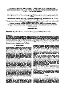
represent gradients of ecosystem parameters at the landscape level, e.g., related to the water cycle, carbon cycle (biomass, NPP), or nutrient cycles (N, P, fiber content, etc.). II. STUDY AREA AND DATA A. Swiss National Park (SNP) Fig. 1. True color composite of a mosaicked APEX scene of upper Val Trupchun acquired on June 24, 2010.

significantly related to water content. Thus, water content represents a measurable parameter that can be used as a surrogate for other plant-related factors that are more difficult to measure. Such quantitative and qualitative vegetation characteristics are, in addition, important factors in affecting trophic interactions between vegetation as food resource and herbivores as the primary consumers, particularly influencing foraging patterns of the latter. We used data of the Airborne Prism EXperiment (APEX) imaging spectrometer [71], collected over the Central European Alps region of the Swiss National Park (SNP), to map the total surface water content of this environment. The specific objectives of this study were 1) to define and apply a methodological framework to assess the ecosystem’s total surface water content on a per-pixel basis; 2) to generate CF maps of two consecutive years to assess temporal variations of total surface water content in the study area; and 3) to assess the potential of linking CF maps to spatial patterns of habitat use of a multispecies ungulate community. Results of this study are considered to serve as a guideline on how IS data, in combination with a method of subpixel assessment of ecosystem properties can support research relying on quantitative information of spatiotemporal dynamics. More specifically, IS allows the simultaneous acquisition of a large number of spectrally continuous bands and therefore provides a wealth of data for optimal land cover class specific assessment of an ecosystem parameter (i.e., total surface water content). We claim to look at several CF simultaneously by separating their information content using spectral mixture analysis (SMA). Attribution of abundances of multiple CF is only possible at high quality with the advent of having high-dimensional data, such as presented. The approach accounts for the complexity of the landscape and incorporates subpixel information into a CF approach. Therefore, it may be useful for habitat assessment to monitor ecosystem responses to environmental change or to

The SNP is located in the south-eastern part of Switzerland and . About are covered by covers an area of vegetation, with forests occupying , alpine grasslands and subalpine grasslands [72], [73]. Elevation ranges from 1350 to 3170 m above sea level (asl). Land cover in the upper Trupchun Valley (Val Trupchun), our specific study area (Fig. 1), is composed of alpine grassland communities distributed over a large gradient of altitude, rocks, and bare soil, snow fields depending on the season and open forest stands of Swiss stone pine and larch (Pinus cembra L./Larix decidua Mill.) up to roughly 2000 m asl. The SNP is the largest protected area in Switzerland and the country’s only national park. It offers a great potential to study ecosystem processes in the absence of human intervention. The Val Trupchun is famous for its exceptionally high densities of chamois (Rupicapra rupicapra L.), ibex (Capra ibex L.) and red deer (Cervus elaphus L.). B. APEX IS Data APEX IS data sets of two consecutive years were collected over the upper Val Trupchun on June 24, 2010 and June 26, 2011. These data sets were part of an attempt to cover large areas of the SNP with APEX IS data on a recurring basis to assess ecosystem processes over time. APEX measures the solar reflected radiance in the wavelength range from roughly 380 to 2500 nm with up to 334 reconfigurable spectral bands in the visible/near infrared (VNIR) and 198 spectral bands in the shortwave infrared (SWIR) spectral region [71]. The pushbroom scanner’s 1000 spatial across track pixels covered a field of view (FOV) of 28 (Table I). The study site was imaged with two flight lines at a flight level of 6500 m asl, resulting in across track pixel sizes ranging from 1.5 to 2.4 m, depending on actual terrain height. The pixel size was resampled to 2 m. Individual flight lines of APEX IS data were geometrically and radiometrically corrected using the PARGE [74] and ATCOR-4 [75] standard approaches. The used parametric geocoding approach reconstructs the scanning geometry of each pixel considering various input data, i.e., boresight information, flight positioning data, and terrain elevation data.

KNEUBÜHLER et al.: CF FROM IMAGING SPECTROMETER DATA FOR ECOSYSTEM PARAMETER MAPPING

TABLE II COUNTS OF LARGE UNGULATE SPECIES GROUPS IN VAL TRUPCHUN IN SUMMER 2010 AND 2011

Noncovered areas were filled by data interpolation using bilinear interpolated gaps. This interpolation method allows preserving the original radiometry in mapped areas and only interpolates data in data gaps. The final pixel size was resampled to 2 m and an evaluation of the resulting geometric accuracy using 15 ground control points revealed a total uncertainty of , which corresponds to a total pixel shift of 1.3–1.9 pixels, pixel. The atmospheric correction approach is based on a precalculated look-up-table, modeled with the atmospheric radiative transfer (RT) code MODTRAN5. The definition of an atmosphere type and an aerosol model (in our case mid latitude summer, and rural aerosol model) in addition with image based estimates of atmospheric water vapor and visibility allows selecting respective LUT entries to compensate atmospheric effects in measured radiance data and to provide top-of-canopy hemispherical conical reflectance factor (HCRF) data. An evaluation of the radiometric performance using three in situ measured surface reflectances of invariant targets revealed an average RMSE of 15% considering the entire wavelength range (data not shown). Subsequent analyses were performed on mosaicked HCRF data (for terminology see [76]). C. Spatial Distribution of Ungulates The SNP’s research department monitored ungulate population sizes and distributions within the park for decades using the same method. On a day with good visibility, the SNP’s park rangers simultaneously mapped the position of all ungulate groups in Val Trupchun, always using the same observation points that overview the entire area. We used animal data collected in summer 2010 and 2011 (Table II) to analyze if there were differences in total surface water content between the grassland areas used by the animals from 1 year to the other. III. METHODS A. Continuous Field Mapping The ecosystem parameter total surface water content was mapped using the proposed CF approach. The CF maps combine subpixel abundance estimates of predominant land cover classes (both vegetated and nonvegetated) in the upper Trupchun Valley (i.e., forest stands, grassland, and rock/soil and snow) and quantitative ecosystem parameters, in this particular case, total surface water content. Land cover abundances of user defined endmembers of forest stands, grassland, rock/soil, and snow were derived using constraint linear SMA [7], [77] over the full set of available APEX bands, and requiring the abundances within a pixel to sum to unity while still allowing abundances to lie below 0 or above 1 [78]. The introduction of a shade

2603

endmember resulted in neglectable impact, most probably due to a high solar zenith angle of 32 during both data acquisitions in 2010 and 2011, and was therefore abandoned. Due to the lack of ground truth in our study, an analysis of the statistics of the residual error image of the SMA provided the only possibility to assess the quality of the resulting land cover abundance maps. Based on discrete classes obtained from an additional maximum likelihood classification of forest stands, grassland, rock/soil, and snow, the class specific RMSE within the SMA error image was assessed. The mean band-wise RMSE values were 1.18% reflectance ( reflectance) for forest areas (dominant abundance), 1.66% reflectance ( reflectance) for grassland areas (dominant abundance), 1.36% reflectance ( reflectance) for soil/rock areas (dominant abundance), and 2.03% reflectance ( reflectance) for snow-covered areas, respectively (2011 data). Water content estimates for the individual land cover types were retrieved from APEX IS data using empirical and physically based approaches (see next section). 1) Water Content Estimation: The water content of the four main land cover types present in Val Trupchun (forest, grassland, rock/soil, and snow) was estimated using spectral indices identified from literature, and a physical approach for the grassland. The main emphasis in this study was to demonstrate the potential of using continuous information synergistically derived from an IS in ecosystem studies rather than fundamentally improving the accuracy of parameter derivation (i.e., water content) from such data itself. Consequently, the choice of indices to estimate the water content of some land cover types might not yet represent the best possible solution, but was considered accurate for our purpose. The identification of more robust approaches to increase the accuracy would need further assessment. The specific index to predict water content of snow-covered areas was the Normalized Difference Snow Index (NDSI) [79]. NDSI was originally developed for the broad spectral bands of LANDSAT TM as [80]

where TM2 and TM5 are LANDSAT TM bands 2 ( μ ) and 5 ( μ ). Accordingly, respective APEX reflectance data were spectrally convolved to match the LANDSAT broadband configuration (refer to [81] for a description of the convolution) and the NDSI was afterwards applied. For our purpose, we assumed that high NDSI values indicate high snow cover, which is in turn related to high water content. In literature, the mean error of subpixel snow cover estimation of NDSI is reported to be less than 10% over the entire range of 0.0–1.0 [79]. For forest stands, water content was related to the Normalized Difference Infrared Index (NDII) [82], which was found to be sensitive to changes in water content of plant canopies. NDII comprises NIR and SWIR spectral information and is defined as [83]

where and are the reflectances at 0.85 and μ , respectively. Wavelengths slightly differ in literature. However,

2604

IEEE JOURNAL OF SELECTED TOPICS IN APPLIED EARTH OBSERVATIONS AND REMOTE SENSING, VOL. 7, NO. 6, JUNE 2014

in this study, APEX spectral bands closest to the indicated NDII bands were used. NDII is reported to be linearly related to canopy moisture with an [82], and linearly related to canopy equivalent water thickness for a large range of land cover classes with an [84]. The estimation of surface soil water content (and potentially on rocks) was based on the Normalized Soil Moisture Index (NSMI) [85] as

where

and are the reflectances at 1.80 and μ , respectively. In our case, APEX spectral bands closest to the indicated NSMI bands were used. A high linear correlation ( , ) between NSMI derived surface soil moisture and field reference data of upper 5 cm soil column is reported in literature [85]. The canopy water content of grassland was retrieved by applying an inversion of the combined one-dimension (1-D) RT models PROSPECT [86] and SAILh [87]. The estimation of vegetation variables using model inversion was based on a lookup-table approach. The leaf level variables chlorophyll content, dry matter content, and water content as well as the canopy parameter LAI were kept free within prior defined ranges and 25 000 combinations were randomly sampled assuming uniform distributions within the defined parameter range. The quasi-inversion minimizes a cost function, which corresponds in our case to the relative RMSE between the measured and the simulated surface reflectance signal, and considers the entire wavelength range from 400 to 2500 nm. The canopy water content was finally calculated as product of the leaf level water content from PROSPECT and the leaf area index estimate from SAILh. In literature, an uncertainty of space based canopy water content estimates of various agricultural crops using an LUT approach is reported as (15%) and [88]. A second study on canopy water content of pioneer vegetation and grassland derived from PROSAIL simulations and subsequent validation with in situ field spectrometer data reports uncertainties of (13.6%) and for a homogeneous site and uncertainties of (14%) and for a heterogeneous site, respectively [89]. Given the consistency of reported uncertainties, we assume similar accuracies in grassland canopy water content in our study. 2) Generation of CF Maps of Total Surface Water Content: The combination of quantitative ecosystem parameters (i.e., total surface water content) and land cover abundance information is the key step to generate the envisaged CF maps (Fig. 2). Essential steps that have to be applied before combining all input data are 1) to scale the water indices values to a common basis and 2) to adjust the SMA derived land cover abundances to be between 0 and 1. The maps of spectral indices (i.e., NDSI, NDII, and NSMI) were linearly scaled to ranges between 0 and 1 [79], [82], [85], thus depicting low to high water content of the respective indices. Land cover abundances with values below 0 or above 1 (as a result of constraint linear SMA with per-pixel abundances summing to unity while allowing values below 0 or above 1) were set to 0 or 1,

Fig. 2. Generation of CF map of total surface water content.

respectively. The spectral indices maps were subsequently multiplied with the corresponding land cover abundance maps. For grassland, the canopy water content map derived from the physical model was multiplied with the grassland abundance values. The final integration of the individual water content maps into a combined product resulted in a map of CF values of total surface water content. This total surface water content map represents water content values in relative units on a per-pixel basis. B. Animal Positions and Water Content To evaluate the spatial distributions of ungulates on grasslands in Val Trupchun and its relation to total surface water content, CF values for total surface water content were extracted for every position of an ungulate group mapped in Val Trupchun in summer 2010 and summer 2011. We investigated the differences in total surface water content between both years for all areas used by the single species (chamois, ibex, and red deer), by the two subfamilies Caprinae Gray (chamois and ibex) and Cervinae Goldfuss (red deer), and by all three species. We also tested for differences in total surface water content between areas used by ungulates (all three species combined) in 2010 and areas they would have used if they were in the positions of 2011, and vice versa. Further, we investigated the differences in total surface water content of areas used by the single species and the two subfamilies when data from the 2 years were combined. We

KNEUBÜHLER et al.: CF FROM IMAGING SPECTROMETER DATA FOR ECOSYSTEM PARAMETER MAPPING

2605

Fig. 4. CF map of relative total surface water content for June 24, 2010. Fig. 3. Subset of a valley slope in Val Trupchun, depicting a true color representation (left), relative total surface water content based on discrete land cover classes (middle) and relative total surface water content based on a CF mapping approach including subpixel abundances of land cover classes (right).

applied the nonparametric Kruskal-Wallis test for all comparisons. For spatial data analysis, we used ArcGIS (version 10.0, Environmental Systems Research Institute, Redlands, CA, US) and for statistical analysis the freeware R (version 2.15.1, R Development Core Team, Vienna, AT). IV. RESULTS A. CF Maps of Total Surface Water Content The advantage of using a CF approach that includes subpixel land cover abundances to map gradients of ecosystem parameters instead of discrete classification approaches is exemplarily shown in Fig. 3 for a subset of a steep valley slope in Val Trupchun. A true color representation (APEX IS data of June 24, 2010) of an area composed of grasslands and soils of varying cover density, as well as rock and snow patches is given in Fig. 3 (left). Relative total surface water content values derived from 1) a mapping approach based on discrete land cover classes and 2) the CF approach as described in Section III-A are shown in Fig. 3 (middle and right), respectively. The discrete approach (Fig. 3, middle) no longer incorporates the subpixel abundance estimates of all present land cover classes but only the dominant class. As a consequence, the respective total surface water content map is subject to a blocky pattern of water content values and continuous gradients are no longer present over distinct land cover borders. The CF map (Fig. 3, right), in contrary, contains smooth gradients across land cover classes and therefore represents the actual situation more realistically. CF maps of relative total surface water content of the upper Val Trupchun for June 24, 2010 and June 26, 2011, respectively (data values between and ) are shown in Figs. 4 and 5. The mean relative value of

Fig. 5. CF map of relative total surface water content for June 26, 2011.

total surface water content amounted to 0.170 for 2010 and to 0.074 for 2011. The availability of multitemporal data sets allowed assessing spatial differences in derived total surface water content between the two dates. Fig. 6 shows the percentage difference in relative total surface water content between the two CF maps of 2010 (Fig. 4) and 2011 (Fig. 5). Roughly 66% of the study area changed less than 5% in relative total surface water content (blueish to reddish colors). Dark blue and dark red denote areas with positive ( > ) and negative differences ( > ) between both years. Large negative differences (red) were mainly found at high altitudes, whereas large positive differences (blue) were predominantly present below the tree line.

2606

IEEE JOURNAL OF SELECTED TOPICS IN APPLIED EARTH OBSERVATIONS AND REMOTE SENSING, VOL. 7, NO. 6, JUNE 2014

Fig. 8. Boxplots for the relative total surface water content of areas used by the three ungulate species (chamois, ibex, red deer) combined in Val Trupchun in summer 2010 and summer 2011. Next to the boxplots for the years (2010, 2011), the boxplots for the water content of the areas the ungulates would have used if they were in the same positions as in the other year are shown (2010_2011: water content of 2010 if the animals were in the 2011 positions, 2011_2010: water content of 2011 if the animals were in the 2010 positions). Horizontal bars represent the median, box heights the interquartile range, and whiskers span interquartile range. Outliers > interquartile range) are not shown. Different letters above the whiskers indicate significant differences ( < ) between the groups. Fig. 6. Difference map (%) of relative total surface water content between values of June 24, 2010 and June 26, 2011, respectively.

Fig. 7. Boxplots for the relative total surface water content of areas used by (a) three ungulate species (chamois, ibex, red deer), (b) two ungulate subfamilies (Caprinae, Cervinae) in Val Trupchun in summer 2010 (i.e., 10) and summer 2011 (i.e., 11), respectively. Horizontal bars represent the median, box heights the interquartile range, and whiskers span interquartile range. Outliers ( > interquartile range) are not shown. Different letters above the whiskers indicate significant differences ( < ) between the groups.

B. Linking the Spatial Distribution of Ungulates to CF Maps No significant yearly differences in total surface water content were found for grassland areas used by the three species [Kruskal-Wallis , , > , Fig. 7(a)] or the two subfamilies [Kruskal-Wallis , , > , Fig. 7(b)]. The yearly difference in total surface water content was significant for areas used by all three species (Kruskal-Wallis , , < , Fig. 8: compare “2010” and “2011”). Considering areas used by all ungulate species in 2010 and potentially used if they were in the same positions as in 2011, no significant differences were obvious (Kruskal-Wallis , , > , Fig. 7 compare “2010” with “2010_2011”). The same applies to areas used by all ungulate species in 2011 and potentially used if they were in the same positions as in 2010

Fig. 9. Boxplots for the relative total surface water content of areas used by (a) three ungulate species (chamois, ibex, red deer) and (b) two ungulate subfamilies (Caprinae, Cervinae) in Val Trupchun in summer 2010 and 2011 combined. Horizontal bars represent the median, box heights the interquartile range, and whiskers span interquartile range. Outliers ( > interquartile range) are not shown. Different letters above the whiskers indicate significant differences ( < ) between the groups.

, , > (Kruskal-Wallis , Fig. 8: compare “2011” with “2011_2010”). When we combined the total surface water content data from 2010 to 2011, we neither found differences between the areas used by the three species [Kruskal-Wallis , , > , Fig. 9(a)], nor between the areas used by two subfamilies [Kruskal-Wallis , , > , Fig. 9(b)]. V. DISCUSSION The concept of using CF allows a realistic representation of ecosystem parameters including their gradients and overcomes limitations of common mapping approaches based on a discretization of land surface properties in classes [16]–[18]. A methodological framework was presented to synergistically derive continuous relative information of total surface water content in an alpine ecosystem dominated by forest stands, grassland, soil/rock, and snow patches from IS data. In vegetated areas, total surface water content was considered as a surrogate of plant

KNEUBÜHLER et al.: CF FROM IMAGING SPECTROMETER DATA FOR ECOSYSTEM PARAMETER MAPPING

TABLE III PHENOLOGICAL INDICATORS RECORDED IN VAL TRUPCHUN FOR AND 2011

THE

YEARS 2010

physiological status. It therefore serves as a proxy to determine potential forage quantity of grasslands, and its predictive power to trace movement patterns of large ungulates was assessed. A. CF of Total Surface Water Content Multitemporal CF maps of total surface water content revealed changes in water content over time. The presented difference map (Fig. 6) shows small-scale, subtle changes of max. 5% mainly in grasslands and, on the other hand, large variations in total surface water content between June 24, 2010 and June 26, 2011 for forested and high elevation areas. For snow-covered areas, large differences in total surface water content between the 2 years are associated with the presence or absence of snow patches in respective areas. Although IS data were acquired on almost identical days of the year (DOY, i.e., June 24 and June 26) in two consecutive years, considerably less snow was present in the high altitudes in 2011 compared to 2010 (dark red areas in Fig. 6). Further, Fig. 6 depicts large positive differences (blue) in total surface water content for forest-covered areas. These differences can be associated with interannual phenological differences in tree development, mainly visible in the development stages of larch (Larix decidua Mill.). Indeed, phenological indicators recorded in Val Trupchun on a regular basis confirm an earlier onset of needle development in both, larch and pine in 2011 (Table III). Further, meteorological data from the MeteoSwiss weather station Buffalora (1980 m asl). i.e., growing degree days with temperatures above 5 C (GDD5) [90], daily total sunshine duration, and daily total precipitation for the period between January to June also suggest differences in the phenological development in both years. GDD5 amounted to 116.5 in 2010 (starting on DOY 114) and to 159.4 in 2011 (starting on DOY 97) from January until the respective dates of APEX data acquisition. The number of days with more than 6 hours of direct sunlight from the first GDD5 to the date of APEX data collection amounted to 19 days (185 h) in 2010 and to 41 days (395 h) in 2011. Total precipitation between January 01 and the date of APEX data acquisition accumulated to 259 mm in 2010 and to 292 mm in 2011. The higher number of GDD5, higher amounts of direct irradiance, and the increased availability of water all suggest that climatic conditions allowed advanced phenological development in spring 2011 compared to 2010. The early onset of the vegetation period in 2011 was probably also a main factor influencing the development of the vegetation later in the season, when an earlier bloom of shrubs (e.g., Rowan Berry, Sorbus aucuparia Michx.), herbs (e.g., Coltsfoot,

2607

Tussilago farfara L.), and grasses (e.g., Dactylis glomerata L.) could be observed (Table III). Besides snow cover and phenological development of trees also shadow effects as a result of different illumination conditions during IS data acquisition might determine differences in total surface water content values between the 2 years. Indeed, IS data were acquired between 09:30 and 10:00 UTC in 2010 and between 12:30 and 13:00 UTC in 2011, causing differences in sun position of sun zenith and sun azimuth within 1 day, and sun zenith and sun azimuth between both data acquisitions. The content of high spatial resolution RS data, including the shadow effect, is known to gain increasing importance in data analysis [91]–[93] and needs further assessment when deriving ecosystem parameters. Maps of total surface water content shown in this study are given in relative units. This is caused by the absence of reference data of absolute water content, which hinders to relate the current relative values to absolute surface water content values. The relative characterization of total surface water content, however, is considered to be sufficient for this first exploration on the applicability of the presented CF concept to represent ecosystem properties synergistically derived from IS data. Further, only a visual validation of the results was possible to ensure that the algorithm did not lead to potentially unrealistic results. A quantitative validation requires extensive efforts considering the water content of all predominant land cover types including a quantitative assessment of their respective abundances. In future work, where maps are intended to be assimilated in e.g., process models, absolute quantifications, and validations are required. B. Relation Between CF Maps and Animal Distribution This study also assessed the suitability of CF maps of ecosystem parameters—in our case total surface water content—to understand animal distribution and grassland habitat use in the SNP. The underlying assumption was that forage quantity or biomass production of grassland can be characterized by the growth limiting factor water. Our results indicate that the spatial distributions of ungulates in summer 2010 and 2011 were not related to the total surface water content of the grassland areas as represented in the respective CF maps. Distinct spatial patterns of habitat use by single species (chamois, ibex, and red deer) and total surface water content in grassland could neither be found within a summer nor between the two summers. The same holds true for ungulate subfamilies (Caprinae and Cervinae). Analysis of both single species and subfamilies data for summer 2010 and 2011 in combination did not reveal specific patterns in habitat use, either. Only the comparison of ungulate positions of all three species were related to significant differences in total surface water content of used grassland patches between 2010 and 2011. A hypothetical combination of summer 2011 animals positions and 2010 total surface water content data (and vice versa) revealed, however, that the same total surface water content (predominantly contained in forage) could have been achieved given the animals had visited the same areas in both years. Given the limited number of observations, these findings could indicate that 1) water availability of the grasslands in Val Trupchun is not a dominant limiting factor for potential forage quantity (biomass)

2608

IEEE JOURNAL OF SELECTED TOPICS IN APPLIED EARTH OBSERVATIONS AND REMOTE SENSING, VOL. 7, NO. 6, JUNE 2014

compared to e.g., temperature, light, and nutrients, or that and 2) ungulates choose their grazing sites based on other criteria. Several studies on plant-herbivore interactions in the SNP have shown competition on forage of highest nutritious quality [73], [94]. With phosphorus (P) being the limiting nutrient in these grasslands, red deer prefer the most P-rich parts for grazing, leading to grazing patterns closely related to patterns of soil-P [94]. Grazing adapted vegetation was found to depict a positive relationship between soil-P and the P concentration in leaf tissues [95]. Consequently, herbivores repeatedly visit specific grazing sites of high nutrients quality rather than forage quantity. This may explain why we could not find differences in grazing patterns between the two summers. Besides, the issue of species competition on popular grazing sites [73] needs further investigation. Since the multitemporal CF maps derived from APEX IS data were found to realistically represent fine-scaled spatiotemporal pattern of ecosystem parameters, it appears promising to continue our analyses of animal distribution patterns in the SNP. We plan to further develop CF maps from IS data for plant biomass, adapt the methodology to other traits, e.g., plant tissue N-content, and acquire ungulate position data on a monthly basis. CF maps of biomass and N-content will enable to characterize the ecosystem in a more detailed way and to test whether grassland areas of high total surface water content do offer high forage quantity and quality. Monthly ungulate positioning data will provide a more robust comparison between the IS data and the spatial distribution of animals.

VI. CONCLUSION In this study, we applied a concept of CF maps synergistically derived from IS data to describe ecosystem properties including their gradients across different land cover types. The continuous representation of total surface water content in a high mountain environment bears the potential for improved assessment and understanding of spatiotemporal dynamics using change-vector analysis. The detailed information contained in CF maps can serve as a spatially explicit input for habitat assessment in ecology. Today, the quality of IS data and the methods for subsequent parameter retrieval do no longer set the limits of vegetationungulates research on plant ecology, but rather on the scarcity of accurate and extensive data on animal habitat use. IS data contain a wealth of spectral information and allow retrieving a variety of biochemical and structural vegetation properties. Such vegetation characteristics can be combined in CF maps to represent a wide range of ecosystem parameters, e.g., related to the water cycle, carbon (biomass, NPP), or nutrients cycles (N, P, etc.). Longer-term multitemporal studies and spatially and temporally improved animal positioning data will help to evaluate the robustness of correlations between ecosystem parameters represented by CF maps and animal distribution patterns in the SNP.

REFERENCES [1] D. M. Muchoney, “Earth observations for terrestrial biodiversity and ecosystems,” Remote Sens. Environ., vol. 112, pp. 1909–1911, 2008. [2] A. Guisan and N. E. Zimmermann, “Predictive habitat distribution models in ecology,” Ecol. Model., vol. 135, pp. 147–186, 2000.

[3] A. K. Skidmore and J. G. Ferwerda, “Resource distribution and dynamics: Mapping herbivore resources,” in Resource Ecology, Spatial and Temporal Dynamics of Foraging, H. H. T. Prins and F. Van Langevelde, Eds. New York, NY, USA: Springer-Verlag, 2008, pp. 57–77. [4] D. W. Bailey et al., “Mechanisms that result in large herbivore grazing distribution patterns,” J. Range Manage., vol. 49, pp. 386–400, 1996. [5] J. M. Fryxell, J. F. Wilmshurst, and A. R. E. Sinclair, “Predictive models of movement by Serengeti grazers,” Ecology, vol. 85, pp. 2429–2435, 2004. [6] S. Ustin, D. A. Roberts, J. A. Gamon, G. P. Asner, and R. O. Green, “Using imaging spectroscopy to study ecosystem processes and properties,” Bioscience, vol. 54, pp. 523–534, 2004. [7] J. W. Boardman, “Automated spectral unmixing of AVIRIS data using convex geometry concepts,” in Proc. Summaries 4th JPL Airborne Geosci. Workshop, Washington, DC, USA, JPL Publication 93-26 V.1, 1993, pp. 11–14. [8] M. E. Schaepman et al., “Earth system science related imaging spectroscopy—An assessment,” Remote Sens. Environ., vol. 113, pp. S123–S137, 2009. [9] B. O. Oindo, A. K. Skidmore, and P. de Salvo, “Mapping habitat and biological diversity in the Maasai Mara ecosystem,” Int. J. Remote Sens., vol. 24, pp. 1053–1069, Jan. 1, 2003. [10] E. Leyequien et al., “Capturing the fugitive: Applying remote sensing to terrestrial animal distribution and diversity,” Int. J. Appl. Earth Observ. Geoinf., vol. 9, pp. 1–20, 2007. [11] X. Feng, B. Fu, X. Yang, and Y. Lü, “Remote sensing of ecosystem services: An opportunity for spatially explicit assessment,” Chin. Geogr. Sci., vol. 20, pp. 522–535, 2010. [12] B. Burkhard, F. Kroll, S. Nedkov, and F. Müller, “Mapping ecosystem service supply, demand and budgets,” Ecol. Indic., vol. 21, pp. 17–29, 2012. [13] R. S. DeFries, J. R. G. Townsend, and M. C. Hansen, “Continuous fields of vegetation characteristics at the global scale at 1-km resolution,” JGR, vol. 104, pp. 16911–16923, 1999. [14] L. Mathys, A. Guisan, T. W. Kellenberger, and N. E. Zimmermann, “Evaluating effects of spectral training data distribution on continuous field mapping performance,” ISPRS J. Photogramm. Remote Sens., vol. 64, pp. 665–673, 2009. [15] R. S. DeFries et al., “Mapping the land surface for global atmospherebiosphere models: Toward continuous distributions of vegetation’s functional properties,” J. Geophys. Res., vol. 100, pp. 20867–20882, 1995. [16] M. Schwarz and N. E. Zimmermann, “A new GLM-based method for mapping tree cover continuous fields using regional MODIS reflectance data,” Remote Sens. Environ., vol. 95, pp. 428–443, 2005. [17] S. L. Ustin and J. A. Gamon, “Remote sensing of plant functional types,” New Phytol., vol. 186, pp. 795–816, 2010. [18] M. C. Levin et al., “Moving from discrete to continuous landscape metrics using remote sensing: The ecological significance of paddock trees for bird richness,” in Proc. Int. Congr. Model. Simul. (MODSIM’07), Dec. 2007, pp. 1342–1348. [19] J. Franklin, “Predictive vegetation mapping: Geographic modelling of biospatial patterns in relation to environmental gradients,” Progress Phys. Geogr., vol. 19, pp. 474–499, 1995. [20] S. Kessell, “Gradient modeling: A new approach to fire modeling and wilderness resource management,” Environ. Manage., vol. 1, pp. 39–48, 1976. [21] R. M. E. A. Hoffer, “Natural resource mapping in mountainous terrain by computer analysis of ERTS-1 satellite data,” Purdue Univ., West Lafayette, IN, USA, Agricultural Experimental Station Research Bulletin 919 and LARS Contract Rep. 061575, 1975. [22] A. H. Strahler, “Stratification of natural vegetation for forest and rangeland inventory using Landsat digital imagery and collateral data,” Int. J. Remote Sens., vol. 2, pp. 15–41, 1981. [23] F. Van Langevelde and H. H. Prins, “Structuring herbivore communities: The role of habitat and diet,” in Resource Ecology, Spatial and Temporal Dynamics of Foraging, H. H. T. Prins and F. Van Langevelde, Eds. New York, NY, USA: Springer-Verlag, 2008, pp. 1–6. [24] N. De Jager and J. Pastor, “Declines in moose population density at Isle Royale National Park, MI, USA and accompanied changes in landscape patterns,” Landscape Ecol., vol. 24, pp. 1389–1403, 2009. [25] J. P. G. M. Cromsigt, H. H. T. Prins, and H. Olff, “Habitat heterogeneity as a driver of ungulate diversity and distribution patterns: Interaction of body mass and digestive strategy,” Diversity Distrib., vol. 15, pp. 513–522, 2009. [26] M. M. Voeten and H. H. T. Prins, “Resource partitioning between sympatric wild and domestic herbivores in the Tarangire region of Tanzania,” Oecologia, vol. 120, pp. 287–294, 1999. [27] T. M. Anderson et al., “Landscape-scale analyses suggest both nutrient and antipredator advantages to Serengeti herbivore hotspots,” Ecology, vol. 91, pp. 1519–1529, May 2010.

KNEUBÜHLER et al.: CF FROM IMAGING SPECTROMETER DATA FOR ECOSYSTEM PARAMETER MAPPING

[28] A. Kittle, J. Fryxell, G. Desy, and J. Hamr, “The scale-dependent impact of wolf predation risk on resource selection by three sympatric ungulates,” Oecologia, vol. 157, pp. 163–175, 2008. [29] K. J. Jenkins and R. G. Wright, “Resource partitioning and competition among cervids in the Northern Rocky Mountains,” J. Appl. Ecol., vol. 25, pp. 11–24, 1988. [30] F. J. Singer and J. E. Norland, “Niche relationships within a guild of ungulate species in Yellowstone National Park, Wyoming, following release from artificial controls,” Can. J. Zool., vol. 72, pp. 1383–1394, 1994. [31] S. Grignolio, I. Rossi, B. Bassano, F. Parrini, and M. Apollonio, “Seasonal variations of spatial behaviour in female Alpine ibex (Capra ibex ibex) in relation to climatic conditions and age,” Ethol. Ecol. Evol., vol. 16, pp. 255–264, 2004. [32] S. Lovari, F. Sacconi, and G. Trivellini, “Do alternative strategies of space use occur in male Alpine chamois?” Ethol. Ecol. Evol., vol. 18, pp. 221–231, 2006. [33] S. Bertolino, N. C. Di Montezemolo, and B. Bassano, “Food–niche relationships within a guild of alpine ungulates including an introduced species,” J. Zool., vol. 277, pp. 63–69, 2009. [34] V. La Morgia and B. Bassano, “Feeding habits, forage selection, and diet overlap in Alpine chamois (Rupicapra rupicapra L.) and domestic sheep,” Ecol. Res., vol. 24, pp. 1043–1050, 2009. [35] J. Schröder and W. Schröder, “Niche breadth and overlap in red deer Cervus elaphus, roe deer Capreolus capreolus and chamois Rupicapra rupicapra,” Acta Zool. Fennica, vol. 172, pp. 85–86, 1984. [36] R. Lande et al., “Estimating density dependence from population time series using demographic theory and life-history data,” Amer. Nat., vol. 159, pp. 321–337, 2002. [37] B.-E. Saether et al., “Stochastic population dynamics of an introduced Swiss population of the ibex,” Ecology, vol. 83, pp. 3457–3465, 2002. [38] B.-E. Saether, M. Lillegård, V. Grøtan, F. Filli, and S. Engen, “Predicting fluctuations of reintroduced ibex populations: The importance of density dependence, environmental stochasticity and uncertain population estimates,” J. Anim. Ecol., vol. 76, pp. 326–336, 2007. [39] B. G. MacKey and D. B. Lindenmayer, “Towards a hierarchical framework for modelling the spatial distribution of animals,” J. Biogeogr., vol. 28, pp. 1147–1166, 2001. [40] M. P. Austin, “Continuum concept, ordination methods, and niche theory,” Annu. Rev. Ecol. Syst., vol. 16, pp. 39–61, 1985. [41] M. P. Austin, “Spatial prediction of species distribution: An interface between ecological theory and statistical modelling,” Ecol. Model., vol. 157, pp. 101–118, 2002. [42] A. Guisan and N. E. Zimmermann, “Predictive habitat distribution models in ecology,” Ecol. Modell., vol. 135, pp. 147–186, 2000. [43] A. Guisan and W. Thuiller, “Predicting species distribution: Offering more than simple habitat models,” Ecol. Lett., vol. 8, pp. 993–1009, 2005. [44] L. Homolová, Z. Malenovský, M. E. Schaepman, G. García-Santos, and J. G. P. W. Clevers, “Review of optical-based remote sensing for plant trait mapping,” Ecol. Complexity, vol. 15, pp. 1–16, 2013. [45] H. Feilhauer, U. Faude, and S. Schmidtlein, “Combining isomap ordination and imaging spectroscopy to map continuous floristic gradients in a heterogeneous landscape,” Remote Sens. Environ., vol. 115, pp. 2513–2524, 2011. [46] H. Feilhauer and S. Schmidtlein, “Mapping continuous fields of forest alpha and beta diversity,” Appl. Veg. Sci., vol. 12, pp. 429–439, 2009. [47] O. N. Krankina et al., “Meeting the challenge of mapping peatlands with remotely sensed data,” Biogeosci. Discuss., vol. 5, pp. 2075–2101, 2008. [48] M. C. Hansen et al., “Towards an operational MODIS continuous field of percent tree cover algorithm: Examples using AVHRR and MODIS data,” Remote Sens. Environ., vol. 83, pp. 303–319, 2002. [49] M. C. Hansen et al., “Continuous fields of land cover for the conterminous United States using Landsat data: First results from the Web-Enabled Landsat Data (WELD) project,” Remote Sens. Lett., vol. 2, pp. 279–288, 2010. [50] M. C. Hansen, R. S. DeFries, J. R. G. Townsend, L. Marufu, and R. Sohlberg, “Development of a MODIS tree cover validation data set for Western Province, Zambia,” Remote Sens. Environ., vol. 83, pp. 320–335, 2002. [51] F. D. S. Cardozo, Y. E. Shimabukuro, G. Pereira, and F. B. Silva, “Using remote sensing products for environmental analysis in South America,” Remote Sens., vol. 3, pp. 2110–2127, 2011. [52] Z. Wu, P. Dijkstra, G. W. Koch, J. Peñuelas, and B. A. Hungate, “Responses of terrestrial ecosystems to temperature and precipitation change: A metaanalysis of experimental manipulation,” Global Change Biol., vol. 17, pp. 927–942, 2011. [53] C. Boisvenue and S. W. Running, “Impacts of climate change on natural forest productivity—Evidence since the middle of the 20th century,” Global Change Biol., vol. 12, pp. 862–882, 2006. [54] H. Rennenberg et al., “Physiological responses of forest trees to heat and drought,” Plant Biol., vol. 8, pp. 556–571, 2006.

2609

[55] J. Kreuzwieser and A. Gessler, “Global climate change and tree nutrition: Influence of water availability,” Tree Physiol., vol. 30, pp. 1221–1234, 2010. [56] T. J. Jackson et al., “Vegetation water content mapping using Landsat data derived normalized difference water index for corn and soybeans,” Remote Sens. Environ., vol. 92, pp. 475–482, 2004. [57] S. S. Choudhary, P. K. Garg, and S. K. Ghosh, “Mapping of agriculture drought using remote sensing and GIS,” Int. J. Sci. Eng. Technol., vol. 1, pp. 149–157, 2012. [58] J. Peñuelas and I. Filella, “Visible and near-infrared reflectance techniques for diagnosing plant physiological status,” Trends Plant Sci., vol. 3, pp. 151–156, 1998. [59] B. Koetz et al., “Radiative transfer modeling within a heterogeneous canopy for estimation of forest fire fuel properties,” Remote Sens. Environ., vol. 92, pp. 332–344, 2004. [60] E. Chuvieco, D. Riaño, I. Aguado, and D. Cocero, “Estimation of fuel moisture content from multitemporal analysis of Landsat Thematic Mapper reflectance data: Applications in fire danger assessment,” Int. J. Remote Sens., vol. 23, pp. 2145–2162, 2002. [61] F. M. Danson and P. Bowyer, “Estimating live fuel moisture content from remotely sensed reflectance,” Remote Sens. Environ., vol. 92, pp. 309–321, 2004. [62] P. Ceccato, S. Flasse, S. Tarantola, S. Jacquemoud, and J.-M. Grégoire, “Detecting vegetation leaf water content using reflectance in the optical domain,” Remote Sens. Environ., vol. 77, pp. 22–33, 2001. [63] B. Datt, “Remote sensing of water content in Eucalyptus leaves,” Aust. J. Bot., vol. 47, pp. 909–923, 1999. [64] H. G. Jones, “Monitoring plant and soil water status: Established and novel methods revisited and their relevance to studies of drought tolerance,” J. Exp. Bot., vol. 58, pp. 119–130, 2007. [65] M. L. Thomey et al., “Effect of precipitation variability on net primary production and soil respiration in a Chihuahuan Desert grassland,” Global Change Biol., vol. 17, pp. 1505–1515, 2011. [66] C. Körner, “Water, nutrient and carbon relations,” in Alpine Treelines. New York, NY, USA: Springer-Verlag, 2012, pp. 151–168. [67] D. S. Wilson and D. A. Maguire, “Environmental basis of soil-site productivity relationships in ponderosa pine,” Ecol. Monogr., vol. 79, pp. 595–617, 2009. [68] H. Yang et al., “Plant community responses to nitrogen addition and increased precipitation: The importance of water availability and species traits,” Global Change Biol., vol. 17, pp. 2936–2944, 2011. [69] K. Djaman, S. Irmak, D. L. Martin, R. B. Ferguson, and M. L. Bernards, “Plant nutrient uptake and soil nutrient dynamics under full and limited irrigation and rainfed maize production,” Agron. J., vol. 105, pp. 527–538, 2013. [70] P. V. V. Prasad, S. A. Staggenborg, and Z. Ristic, “Impacts of drought and/ or heat stress on physiologial, developmental, growth, and yield processes of crop plants,” in Response of Crops to Limited Water, L. R. Ahuja, Ed. Madison, WI, USA: American Society of Agronomy, 2008, pp. 301–356. [71] M. Jehle et al., “APEX—Current status, performance and product generation,” in Proc. IEEE Sens. Conf., Waikoloa, HI, USA, Nov. 1–4, 2010, pp. 533–537. [72] A. C. Risch, M. F. Jurgensen, D. S. Page-Dumroese, O. Wildi, and M. Schütz, “Long-term development of above- and belowground carbon stocks following land-use change in subalpine ecosystems of the Swiss National Park,” Can. J. Forest Res., vol. 38, pp. 1590–1602, 2008. [73] M. Schütz, A. C. Risch, E. Leuzinger, B. O. Krüsi, and G. Achermann, “Impact of red deer (Cervus elaphus L.) on patterns and processes on subalpine grasslands in the Swiss National Park,” Forest Ecol. Manage., vol. 181, pp. 177–188, 2003. [74] D. Schläpfer and R. Richter, “Geo-atmospheric processing of airborne imaging spectrometry data. Part 1: Parametric orthorectification,” Int. J. Remote Sens., vol. 23, pp. 2609–2630, 2002. [75] R. Richter and D. Schläpfer, “Geo-atmospheric processing of airborne imaging spectrometer data. Part 2: Atmospheric/topographic correction,” Int. J. Remote Sens., vol. 23, pp. 2631–2649, 2002. [76] G. Schaepman-Strub, M. E. Schaepman, T. H. Painter, S. Dangel, and J. V. Martonchik, “Reflectance quantities in optical remote sensing— Definitions and case studies,” Remote Sens. Environ., vol. 103, pp. 27–42, 2006. [77] J. W. Boardman, “Inversion of high spectral resolution data,” in Proc. SPIE, 1990, vol. 1298, pp. 222–233. [78] F. Van Der Meer and S. M. De Jong, “Improving the results of spectral unmixing of Landsat Thematic Mapper imagery by enhancing the orthogonality of end-members,” Int. J. Remote Sens., vol. 21, pp. 2781–2797, 2000. [79] V. V. Salomonson and I. Appel, “Estimating fractional snow cover from MODIS using the normalized difference snow index,” Remote Sens. Environ., vol. 89, pp. 351–360, 2004.

2610

IEEE JOURNAL OF SELECTED TOPICS IN APPLIED EARTH OBSERVATIONS AND REMOTE SENSING, VOL. 7, NO. 6, JUNE 2014

[80] J. Dozier, “Spectral signature of alpine snow cover from the Landsat Thematic Mapper,” Remote Sens. Environ., vol. 28, pp. 9–22, 1989. [81] P. D’Odorico, A. Gonsamo, A. Damm, and M. E. Schaepman, “Experimental evaluation of Sentinel-2 spectral response functions for NDVI timeseries continuity,” IEEE Trans. Geosci. Remote Sens., vol. 51, no. 3, pp. 1336–1348, Mar. 2013. [82] M. A. Hardisky, V. Klemas, and R. M. Smart, “The influences of soil salinity, growth form and leaf moisture on the spectral reflectance of Spartina alterniflora canopies,” Photogramm. Eng. Remote Sens., vol. 49, pp. 77–83, 1983. [83] M. T. Yilmaz, E. R. Hunt, Jr., and T. J. Jackson, “Remote sensing of vegetation water content from equivalent water thickness using satellite imagery,” Remote Sens. Environ., vol. 112, pp. 2514–2522, 2008. [84] M. T. Yilmaz et al., “Vegetation water content during SMEX04 from ground data and Landsat 5 Thematic Mapper imagery,” Remote Sens. Environ., vol. 112, pp. 350–362, 2008. [85] S.-N. Haubrock, S. Chabrillat, M. Kuhnert, P. Hostert, and H. Kaufmann, “Surface soil moisture quantification and validation based on hyperspectral data and field measurements,” J. Appl. Remote Sens., vol. 2, no. 1, 023552, 2008, doi:10.1117/1.3059191. [86] S. Jacquemoud and F. Baret, “PROSPECT: A model of leaf optical properties spectra,” Remote Sens. Environ., vol. 34, pp. 75–91, 1990. [87] W. Verhoef, “Light scattering by leaf layers with application to canopy reflectance modeling: The SAIL model,” Remote Sens. Environ., vol. 16, pp. 125–141, 1984. [88] J. Cernicharo, A. Verger, and F. Camacho, “Empirical and physical estimation of canopy water content from CHRIS/PROBA data,” Remote Sens., vol. 5, pp. 5265–5284, 2013. [89] J. G. P. W. Clevers, L. Kooistra, and M. E. Schaepman, “Estimating canopy water content using hyperspectral remote sensing data,” Int. J. Appl. Earth Observ. Geoinf., vol. 12, pp. 119–125, 2010. [90] L. Moser et al., “Timing and duration of European larch growing season along altitudinal gradients in the Swiss Alps,” Tree Physiol., vol. 30, pp. 225–233, 2010. [91] C. E. Woodcock and A. H. Strahler, “The factor of scale in remote sensing,” Remote Sens. Environ., vol. 21, pp. 311–332, 1987. [92] G. P. Asner and A. S. Warner, “Canopy shadow in IKONOS satellite observations of tropical forests and savannas,” Remote Sens. Environ., vol. 87, pp. 521–533, 2003. [93] P. M. Dare, “Shadow analysis in high-resolution satellite imagery of urban areas,” Photogramm. Eng. Remote Sens., vol. 71, pp. 169–177, 2005. [94] M. Schütz et al., “Phosphorus translocation by red deer on a subalpine grassland in the central European Alps,” Ecosystems, vol. 9, pp. 624–633, 2006. [95] C. Thiel-Egenter et al., “Response of a subalpine grassland to simulated grazing: Aboveground productivity along soil phosphorus gradients,” Community Ecol., vol. 8, pp. 111–117, 2007. Mathias Kneubühler received the M.S. degree in geography and the Ph.D. degree (Dr. sc. nat.) in remote sensing with emphasis on spectral assessment of crop phenology, both from the University of Zürich, Zürich, Switzerland, in 1996 and 2002, respectively. He is currently the Head of the Spectroscopy Laboratory of the Remote Sensing Laboratories (RSL), University of Zurich. His research interests include spectro-directional data analysis and spectral assessment of phenological processes in vegetated ecosystems. Alexander Damm received the Diploma (M.Sc.) and Ph.D. degrees in geography from the Humboldt University, Berlin, Germany, in 2004 and 2008, respectively. From December 2008 to 2012, he was as a Postdoctoral Researcher and since 2012, he has been a Lecturer with the Remote Sensing Laboratories, University of Zürich, Zürich, Switzerland. He acted as the responsible Project Manager for the largest APEX (Airborne Prism Experiment) exploitation program aiming at supporting advanced product development using spectroscopy-based approaches. Currently, he is responsible for the Swiss Earth Observatory Network (SEON), a competence center to monitor status and functioning of ecosystems in a changing environment. His research interests include Earth observation, with particular focus on biosphere-atmosphere interactions and ecosystem functioning using imaging spectroscopy.

Anna-Katharina Schweiger received the B.Sc. degree in biodiversity and ecology from the University of Graz, Graz, Austria, in 2007, and the M.Sc. degree in wildlife ecology from the University of Natural Resources and Life Sciences, Vienna, Austria, in 2010. Currently, she is pursuing the Ph.D. degree in grassland ecology at the Remote Sensing Laboratories, University of Zurich, Zurich, Switzerland. She works in close collaboration with the PlantHerbivore Interactions Group, Swiss Federal Institute for Forest, Snow and Landscape Research WSL, Birmensdorf, Switzerland, and with the Swiss National Park, Zernez, Switzerland, where she holds a position with the Research and Geoinformation Department. Her research interest is on the analysis of animal tracking data with remote sensing techniques.

Anita C. Risch received the M.Sc. degree in biology from the Swiss Federal Institute of Technology (ETHZ), Zurich, Switzerland, in 1999, the M.Sc. degree in forest ecology from Michigan Technological University (MTU), Houghton, MI, USA, in 2000, and the Ph.D. degree in ecology, from ETHZ, in 2004. From 2004 to 2006, she spent her Postdoctoral time with Syracuse University, Syracuse, NY, USA. In 2006, she became the Head of the Animal Ecology Research Group, Swiss Federal Institute for Forest, Snow and Landscape Research (WSL), Birmensdorf, Switzerland. Since 2008, she has been a Graduate Faculty and Adjunct Associate Professor at MTU and completed her habilitation at ETHZ in 2010. She currently leads the Plant-Animal-Interaction Research Group at WSL. Her research interests include how vertebrate and invertebrate animals affect above- and belowground ecosystem processes.

Martin Schütz received the M.Sc. and Ph.D. degrees in biology from the Swiss Federal Institute of Technology (ETHZ), Zurich, Switzerland, in 1983 and 1988, respectively. Since 1994, he was the Leader of several research groups with the Swiss Federal Institute for Forest, Snow and Landscape Research (WSL), Birmensdorf, Switzerland, and became the Senior Scientist in 2006. Since 2008, he has been the Adjunct Professor with Michigan Technological University (MTU), Houghton, MI, USA, and a Member of the Board of Science of the Swiss National Park. His research interests include assessing vegetation dynamics and interactions between plants and animals.

Michael E. Schaepman (M’05–SM’07) received the M.Sc. and Ph.D. degrees in geography from the University of Zuürich (UZH), Zuürich, Switzerland, in 1993 and 1998, respectively. In 1999, he spent his Postdoctoral time with the Optical Sciences Center, The University of Arizona, Tucson, AZ, USA. In 2000, he was appointed as a Project Manager of the European Space Agency Airborne Prism Experiment Spectrometer. In 2003, he accepted the position of Full Chair of Geoinformation Science and Remote Sensing, Wageningen University, Wageningen, The Netherlands. In 2009, he was appointed as the Full Chair of Remote Sensing, UZH, where he is currently heading the Remote Sensing Laboratories, Department of Geography. His research interests include computational Earth sciences using remote sensing and physical models, with particular focus on the land–atmosphere interface using imaging spectroscopy.