Continuous Gaussian Mixture Modeling - CiteSeerX

Printed in Proceedings of the Information Processing for Medical Imaging Conference, Ed. James Duncan, Vermont, 1997. 14 Pages

Continuous Gaussian Mixture Modeling Stephen Aylward1 and Stephen Pizer2 1Department of Radiology 2Department of Computer Science

Medical Image Display and Analysis Group University of North Carolina Chapel Hill, NC 27599

Abstract. When the projection of a collection of samples onto a subset of basis feature vectors has a Gaussian distribution, those samples have a generalized projective Gaussian distribution (GPGD). GPGDs arise in a variety of medical images as well as some speech recognition problems. We will demonstrate that GPGDs are better represented by continuous Gaussian mixture models (CGMMs) than finite Gaussian mixture models (FGMMs). This paper introduces a novel technique for the automated specification of CGMMs, height ridges of goodness-of-fit. For GPGDs, Monte Carlo simulations and ROC analysis demonstrate that classifiers utilizing CGMMs defined via goodness-of-fit height ridges provide consistent labelings and compared to FGMMs provide better truepositive rates (TPRs) at low false-positive rates (FPRs). The CGMM-based classification of gray and white matter in an inhomogeneous magnetic resonance (MR) image of the brain is demonstrated.

1 Introduction The crux of statistical pattern recognition and data analysis is the accurate modeling of the distributions of data. This paper presents a novel technique which is ideally suited for representing GPGDs. GPGDs arise in a variety of medical images such as MR images containing intensity inhomogeneities, X-ray CT images due to beam hardening, and SPECT images due to deficiencies in attenuation compensation. GPGDs also exist in some speech and handwriting recognition problems. It has been demonstrated that within small regions of an MR image, a tissue’s intensity will be Gaussian distributed, yet the parameters of those localized Gaussian distributions will vary as a result of an intensity inhomogeneity. Consider the proton density (PD) MR image in Fig. 1. It was acquired and converted to byte pixel values as described in [2]. It contains an intensity inhomogeneity which exists as a large scale dimming in the inferior cerebellum. The inhomogeneity can be quantified (Fig. 2) by Gaussian blurring the image at a scale of 15 pixels using only those pixel’s having values between 100 and 200. More exact methods for measuring the inhomogeneity exist [4, 10, 16], but the stated approach is sufficient for our demonstration. The correlation between PD value and inhomogeneity

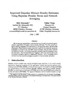
Fig. 1. Proton density MR image

Fig. 2. Estimated intensity inhomogeneity

Magnitude Inhomogeneity Estimated Local Mean PD Value


200

Gray Matter "grey.pdgf_15.data" "white.pdgf_15.data" White Matter

180 160 140 Generalized Projective Gaussians 120 100 100

150 PD Value

200

Fig. 3. Scatterplot of hand-labeled gray and white matter samples

magnitude is revealed by a scatterplot (Fig. 3) formed from 984 hand-labeled white matter and 788 gray matter samples from these images. In that scatterplot, every local collection of a tissue’s samples has a Gaussian distribution, but a continuum of Gaussians is needed t o represent each tissue’s entire distribution; the distributions are GPGDs. In speech recognition, it is commonly accepted that hidden Markov models using Gaussian distributions can represent certain aspects of the speech of a single person in a controlled situation, e.g., given a fixed level of stress. Smooth warpings can be applied t o the parameters of those Gaussians to transition them to new situations and speakers [3] . To account for such variations in speaker and situation, multiple Gaussians are needed; the distributions resemble GPGDs. When the correlations creating the GPGDs are well understood and easily measured, the most accurate models can be obtained by directly eliminating their effects and then using simple Gaussians [4, 10, 16] . When the correlations are not well understood or easily measured, Gaussian mixture models are appropriate. Traditionally, FGMMs defined via maximum likelihood expectation maximization (MLEM) have been used to represent GPGDs. We will show that these distributions are more accurately and consistently represented by continua of means and variances. We call such continua "traces." We will show that the traces of a sampled GPGD can be extracted via height ridges of goodness-of-fit functions, and that these traces accurately and consistently define a CGMM of the underlying GPGD. For this paper, the accuracy and consistency of the distribution models are quantified b y the accuracy and consistency of the classifiers they define. That is, when a model Ψ of a class i is used to provide class conditional probability estimates P(x | Ψ(i)) to a classifier, the accuracy and consistency of the labelings produced by that classifier determine the accuracy and consistency of the model. Assuming equal class priors P(Ψ(i)) and maximum likelihood Bayes Rule classification, then

( )

  P Ψ i P x Ψ i    label for x = ARGMAX P Ψ i x = = P x Ψ i   i=1..# of classes P x ( )    

( )

[1]

A classifier’s labeling accuracy is quantified by its TPRs and FPRs, and its labeling consistency is the standard error of those rates. Section 2 introduces finite and continuous Gaussian mixture modeling. Section 3 presents our implementation of goodness-of-fit functions. These functions respond maximally when their parameters µ´ and σ´ match those of the distribution from which the samples being tested originated. That section also discusses the how these functions are applied normal to the trace of a GPGD in order to extract that trace using a height ridge


definition, and it ties the traces to the definition of a CGMM. Section 4 uses GPGDs, Monte Carlo simulations, and ROC analysis to compare FGMMs with CGMMs. Section 5 demonstrates the CGMM-based classification of tissues in an inhomogeneous MR image.

2 Gaussian Mixture Modeling A mixture model is formed using multiple “component” distributions. In a Gaussian mixture model the component distributions are multivariate (N-dimensional) normal densities each of which is parameterized by φ.

F(x;Φ ) =

2.1

( )

(2 π )N 2 Σ

12

( )

t 1 x − µ Σ −1 x − µ 2 e

−

1

where

{ }

Φ = µ, Σ

[2]

Finite Gaussian Mixture Modeling

If the number of components K is bounded, the Gaussian mixture model is a FGMM Ψ. It provides a probability for a sample x via

(

K

)

K

P(x Ψ ) = ∑ ω (i) F x;Φ (i) where 1 = ∑ ω ( i ) and Ψ = i =1

i =1

{{ω,Φ}(i)

}

i = 1..K

[3]

Most investigations involving mixture models use FGMMs trained via MLEM. While n o FGMM training algorithm is best in all situations, MLEM is easy to implement and provides several desirable convergence properties such as monotonic convergence [5, 7, 8 , 18]. MLEM, however, is an approximate gradient ascent algorithm, and it is subject t o non-optimal local and global maxima. While MLEM is relatively robust to these nonoptimal maxima [7, 15, 18], it will be shown that the FGMM component parameterizations produced via MLEM can vary greatly and be far from optimal given different sets of samples from the same distribution; FGMMs offer poor consistency. This inconsistency i s aggravated by the reliance on the user to specify the number of components. While much research has focused on automatically determining an appropriate number of components for a given problem, a generally applicable approach has not be found [9, 18]. A FGMM’s expected accuracy does not vary monotonically as a function of the number of components. Additionally, MLEM’s non-optimal maxima can lead to poorly utilized components; the effective number of components in an FGMM may be less than the user specified number of components. GPGDs are comprised of an infinite number of components, so determining an appropriate finite number of components to approximate them with can be especially difficult. 2.2

Continuous Gaussian Mixture Modeling

A continuous mixture model consists of an uncountably infinite number of components whose parameters Ψ span Nt traces T(j) through the parameter space of its components, i.e., the domain of φ. A CGMM provides a probability via

 ∃ j ∈1..N t s.t . Φ ∈ T( j)  P(x Ψ ) = MAX ω F(x;φ ) where Ψ = {ω , Φ }  {ω ,φ }∈Ψ and ω = P(Φ )  

(

)

[4]

This equation follows the simplifying assumptions made by Dempster, Laird, and Rubin [5] and states that since the underlying distribution is assumed to be a mixture, each sample i s in fact generated by just one of the infinite number of components, the generating component is determined via maximum likelihood, and the generating component provides


the best estimate of the sample’s probability. The function F(x ;φ) can be interpreted as providing a trace point conditional sample probability, and ω as providing a trace point a priori probability. Equation 3 can therefore be rewritten as [5] P( x Ψ ) = MAX P(Φ )P(x Φ ) Φ ∈T( j) ∈Ψ j∈1.. N t

(

)

The focus of this paper is the definition of the traces T (j) via height ridges of goodnessof-fit functions. A CGMM defined in this manner can accurately and consistently model the continua of means and variances which form a GPGD. For this paper, analysis is limited t o GPGD’s having one-dimensional traces.

3 Traces of Goodness-of-Fit Each trace of a GPGD can be viewed as a continuum of central means (centers) with smoothly changing variances normal to that continuum (widths). A method has already been developed for representing the centers and widths of objects. That object representation method is known as the medialness core [12]. Medialness cores have been proven to be invariant to rotation, translation, intensity, and scale [12] and insensitive t o a wide variety of image and boundary noise [11]. To apply medialness core methods to the representation of distributions, goodness-of-fit functions are used instead of medialness functions because goodness-of-fit functions are sensitive to sample density whereas medialness functions are sensitive to boundariness. 3.1.

Univariate

Gaussian

Goodness-of-Fit

One class of goodness-of-fit functions is the univariate chi-squared measures. This class includes Pearson’s statistic χ 2P , Read and Cressie’s power divergent statistic χ 2R &C , and the log likelihood ratio χ 2LLR [14]. Since our goal is to develop mixture models using Gaussian components, the binned expected distribution E of these omnibus measures i s derived from a univariate Gaussian. These functions are therefore referred to as Gaussian goodness-of-fit (GGoF) functions. The parameters of these functions are µ´ and σ´, the mean and standard deviation to be tested; µ´ and σ´ define the expected distribution E. This paper uses six bins B=6 centered at µ´ and clipped so as to capture samples within ±1.645σ´ of µ´. The GGoF functions are devised so as to be maximal when their parameters µ´ and σ´ best match the µ and σ of the population from which the samples originated. This is achieved by subtracting the standard goodness-of-fit functions from χ 62 −1 (α = 0.99) = 15.09 and then normalizing b y that value (Equation 6). As a result of these modifications, a GGoF function’s value i s expected to be greater than zero for 99% of the sets of samples which originate from a Gaussian parameterized by µ´ and σ´.

 B  O  χ 2LLR (µ' , σ') = 15.09 − 2 ∑ O i ln i   / 15.09  Ei   i =1 

[6]

The accuracy and consistency of the local maxima of the χ 2P , χ 2R &C , and χ 2LLR GGoF functions were evaluated using 96 Monte Carlo simulations. Each simulation consisted of 5000 runs. The simulations considered four different training set sizes (20, 40, 80, 160 samples) from two distributions (a Gaussian with µ=128 and σ=16 and a log-normal distribution using a log base of 1.6) and four different binning techniques (equirange, equiprobable, overlapped-equirange, overlapped-equiprobable) [1]. For each Monte Carlo run, the local maximum of the GGoF function was found via gradient ascent through (µ´, σ´). The starting points for gradient ascent were selected from a 2D Gaussian distribution


centered at each population’s ideal parameter values (µ, σ) having a standard deviation of 5% of those values. The accuracy of a local GGoF maximum was defined as the difference between the GGoF parameters (µ´, σ´) of that maximum and the population’s actual parameters (µ, σ). Consistency was calculated as the standard error associated with each parameter µ´ and σ´ of the maxima from each simulation. Conclusions drawn include that 1) the binning method has more influence on accuracy and consistency than the GGoF function; 2) the accuracy and consistency of the estimates of µ do not vary significantly as a function of the number of samples, the GGoF function, or the binning technique; 3) χ 2LLR with overlapped-equiprobable binning provides the most accurate and consistent estimates σ. As a result, χ 2LLR with overlapped-equirange binning was used for all GGoF trace calculations. 3.2

Multivariate GGoF via Trace Tangents and Normals

To calculate multivariate GGoF values, the multivariate data about a given µ´ are converted to multiple univariate distributions via projection onto a set of basis directions. The expected variance associated with each of those projections may differ. The multivariate GGoF value is the average χ 2LLR value from each of those projections. We hypothesize that neighboring GGoF trace points capture a distribution’s variance in the trace tangent direction, so each trace point needs only to capture variance normal to the trace. To estimate a trace’s normal (and tangent) directions as well as the expected variance of the distribution in each of those directions, our algorithm extends the geometric measures via statistics work conducted by Yoo [17]. Specifically, we suggest that eigenvectors of the local data’s covariance matrix ∑(L) well approximate the normal (and tangent) directions of the GGoF trace, and the eigenvalues define expected variance ratios for each of the normal directions. Since ∑(L) is a function of only two variables, i.e., a mean µ´ and a neighborhood size s´, its use in calculating multivariate GGoF functions allows those functions to be parameterized by just µ´ and s´. ∑(L) approximation of the tangent allows a GGoF trace to be traversed without derivative calculations. ∑(L) is measured using a Gaussian weighting G(•) of the samples S about µ´ so as t o change smoothly given small changes in µ´ or s´.

(

)

(

)(

)(

Σ ( L ) µ' , s' = ∑ G z µ' , 3s' z i − µ' i z j − µ' j ij z∈S

)

(

∑ G y µ' , 3s'

y∈S

)

[7]

Define λi for i=1..N as the descending ordered eigenvalues of ∑(L) and v i as their corresponding eigenvectors. If no additional information is available, it can be assumed that the maximum eigenvalued eigenvector v 1 approximates the GGoF trace’s tangent direction. The remaining eigenvectors specify the normal directions. Expected variances in each of the normal directions are specified by eigenvalue ratios; the expected variance i n the eigen-direction, v i | i=2..N, is (σ´)2 = (s´)2λi/λ2. To help understand the N+1 dimensional GGoF “space” (µ´, s´) of an N dimensional distribution, slices through the 3D GGoF space of a 2D distribution in (f0,f1) can be calculated. Consider the scattergram shown in Fig. 4. Those 900 samples were generated from a simulated GPGD, Class A. Class A is defined by three approximating cubic Bsplines and four isotropic control Gaussians (Table 1). Each spline governs one of the three parameters of the Gaussians, i.e., f0, f1, σ. To generate a sample, a parametric value t is chosen from the uniform distribution U[0,1]. The three splines are evaluated at that t value, an isotropic Gaussian distribution is thus defined, and from that distribution the sample is then generated. Figs. 5-7 are the GGoF values for fixed s´ and a range of µ´ values using the samples in Fig. 4. 1D GGoF traces appear along the extent of the distribution.


G(0) G(1) G(2) G(3)

Mean f0 80 112 144 192

σ 16 1 1 16

f1 112 56 56 112

Table 1. Control Gaussian of the GPGD, Class A 255

255

f1

f1

0

0 0

f0

255

Fig. 4. Scattergram of 900 Class A samples 255

255

f1

f1

0

0

255 f 0 Fig. 6. Class A’s GGoF space at s´=8 0

3.3

0 255 f 0 Fig. 5. Class A’s GGoF space at s´=4

0 255 f 0 Fig. 7. Class A’s GGoF space at s´=16

Gaussian Goodness-of-Fit Trace Extraction

As mentioned previously, GGoF traces are based on medialness cores. Techniques developed for medialness core extraction are used to extract GGoF traces. The three steps involved are trace stimulation, traversal, and traversal termination. Trace Stimulation. A trace stimulation point has two components, µ0 and s 0 . FGMM is used to specify µ0. Specifically, the user must select the number of FGMM components to use, the data are then modeled using FGMM, and the component mean which is nearest (measured via Euclidean distance) to two other component means is chosen as µ0. As a result, µ0 will generally be located within a dense region of a sampled GPGD. If multiple traces are requested, the remaining component means are used. The number of FGMM components used appears to be non-critical; for all CGMMs developed in this paper the stimulating FGMM used 7 components. Specifying s0 reduces to determining an initial neighborhood size for calculating ∑(L) at µ0. By assuming that the trace tangent at µ0 is well approximated by the maximum eigenvalued eigenvector of ∑(L), s0 is the square root of the second largest eigenvalue. For this paper, the initial neighborhood size is set equal to the distance between µ0 and its


closest neighboring FGMM mean. s 0 =17.94.

For the data in Fig. 4, µ0 =(163.66, 80.08) and

Trace Traversal. The trace normals are approximated by the non-tangent eigenvectors of ∑(L) and a unit vector which points strictly in s. These directions define a hyperplane i n GGoF space through which the local trace segment passes. When this normal plane i s slightly shifted in the local trace tangent direction, a gradient ascent with respect to the GGoF values within that plane leads to a new trace point. For this paper, a step size of 0.1 feature space units is used to shift the normal plane, gradient ascent within that shifted plane is performed using Brent’s line search method [13], and gradient ascent terminates when the gradient’s projection onto the plane is less than 0.1% of its total magnitude. The point in the plane at which gradient ascent terminates is the new trace point. The new tangent direction is approximated by the eigenvector of local data’s covariance matrix that has the maximum magnitude dot product with the previous trace point’s tangent eigenvector. If the sign of the dot product is negative, the new tangent vector is negated t o maintain the direction of traversal. This process is repeated until a traversal termination criterion is met. Trace Traversal Termination and Recovery. Trace traversal terminates when a “well fitting” Gaussian cannot be found. Empirical evidence suggests that encountering a GGoF value of -10 or less is a reasonable stopping criterion. This criterion was used t o terminate the traversal of every trace presented in this paper. The rate of change of the trace is used to identify suspect trace points and halt their inclusion into the trace without causing termination of the traversal process. Such points are “stepped over” using the tangents of the previous valid trace point. The µ´ component of a 1D GGoF trace of the data in Fig. 4 is shown in Fig. 8. The effect of recovery is visible as a break in the trace. To visualize the normal variance estimates provided by the trace, the 0, ±0.5, ±1, ±1.5, and ±2 σ´ points along the normal at each trace point can be plotted (Fig. 9). The next section details the conversion of a GGoF trace to a CGMM. 255

250

Samples Core

200

f1

f1

150 100 50

0

0 0

100

200 f0

Fig. 8. µ´ of a GGoF trace of Fig. 4

3.4

0

f0

255

Fig. 9. Isocontours of the variance estimates

CGMMs via GGoF Traces

As defined in Equation 4, two values, P(x |φ) and P(φ ), are required at each trace point φ t o define a CGMM Ψ. To calculate P(x |φ ), a trace point covariance matrix ∑(φ) must be defined. The eigenvectors and eigenvalues of ∑(φ) are defined by 1) the approximate normal directions and expected variances which were used to calculate φ''s GGoF value (Section 3.2)


and 2) the approximate tangent direction which is assigned a variance equal to the maximum expected variance in a normal direction. A trace point’s a priori probability P(φ) is defined as the portion of samples it i s expected to represent. The expected number of samples that will be represented by a trace point can be extrapolated based on the number of observed samples within a fixed standard deviation, i.e., s, of that point. The CGMM defined via the GGoF trace depicted in Figs. 8 and 9 produces the probability density function depicted Fig. 10. Although the GGoF trace extended beyond the distribution, the low prior probabilities P(φ) associated with those points reduce the negative effects of the over extension. The estimated density function should be compared with the population’s actual density function which is shown in Fig. 11. There appears t o be good correspondence. The next section focuses on quantifying that correspondence. 255

255

f1

f1

0

0 0

f0

255

Fig. 10. CGMM estimated probability density function of Class A

0 255 f 0 Fig. 11. Actual probability density function of Class A

4 CGMM’s Accuracy and Consistency To determine the accuracy and consistency of a classifier and thereby determine the accuracy and consistency of the distribution models it uses, Monte Carlo simulations and ROC analyses must be performed. This section begins by presenting an example classification result. 4.1

Example

Results

The accuracy and consistency of a modeling technique is being determined by the accuracy and consistency of the labelings produced by classifiers that use the probability estimates provided by those models. Class A was defined in Section 3.2. A competing class, Class B, is defined as an isotropic Gaussian with µ=(128,128) and σ=36. Given the set of 900 training samples from Class B, the stimulation point µ0 =(160.37, 123.30) and s0 =17.94 is automatically chosen. The resulting trace point conditional isoprobability curves overlaid onto the training data scattergram are shown in Fig. 12. Using the Class A and Class B models developed thus far, every point in feature space can be assigned a label and an image can be developed which reflects those labelings with differing shades of gray. Fig. 13 i s such an image with the optimal decision bounds between the classes overlaid in black. The CGMMs of Classes A and B provide accurate labelings for the majority of feature space. To improve the CGMM’s labelings, multiple traces can be used. While generally containing redundant information, additional traces do refine a CGMM. CGMMs using 7 traces per class (CGMM07) produce the labelings shown in Fig. 14. FGMMs using 7 components per class (FGMM07) produce the labelings shown in Fig. 15. Allocation t o


255

255

f1

f1

0

0 0

f0

255

Fig. 12. Isoprobability curves of Class B’s CGMM

0

f0

255

Fig. 13. Labeling of feature space produced by CGMMs with optimal decision bound overlaid

255

255

f1

f1 Poorly utilized FGMM component

0

0 0

f0

0

255

f0

255

Fig. 14. Labelings by CGMM07 Fig. 15. Labelings produced by FGMM07 Different shades of gray correspond to allocation to different traces/components. Light gray shades indicate assignment to Class A

each trace/component is indicated by different shades of gray; light grays indicate allocation to Class A. The presence of non-optimal FGMM maxima is clear; one Class A component is reduced to representing a sliver through feature space. That component i s being poorly utilized, and its use does not correspond with the underlying distribution. Given 2700 testing samples from each class, the Class A TPRs and FPRs in Table 2 , Run1 are produced. Compared to FGMM07, CGMM07 offers an 718% decrease in the FPR with a less than 11% decrease in the TPR! To determine if these results were anomalous, new models were developed and tested using different samples from Classes A and B. Those results are summarized in Table 2, Run2. CGMM07 again produced the lowest FPR, but the differences are less dramatic. While no conclusions should be drawn from these two runs, the results are quite encouraging. Not only does CGMM07 provide the lowest FPR values and competitive TPR

CGMM01 CGMM02 CGMM04 CGMM07 FGMM01 FGMM02 FGMM04 FGMM07

Run1 FPR 0.3233 0.3215 0.2604 0.0385 0.2933 0.3259 0.3315 0.3152

TPR 0.8859 0.8859 0.8367 0.8237 0.8415 0.9196 0.9259 0.9130

Run2 FPR 0.2281 0.2178 0.2200 0.2318 0.2878 0.3185 0.3218 0.3067

TPR 0.6681 0.7874 0.8204 0.8485 0.8659 0.9307 0.9400 0.9141

Table 2. Class B TPRs & FPRs from two different sets of training and testing data


values, but there is also an ordered progression in the TPR & FPR values for CGMM as the number of traces used is increased. For FGMM, the use of additional components does not always increase performance. 4.2

Monte Carlo Results

To gain an understanding of the expected consistency with which CGMMs model GPGDs, Monte Carlo simulations involving Class A and Class B were performed. Initial simulations revealed that even after 5000 repetitions of the modeling and testing task of Section 4.1, classifiers using FGMMs demonstrated extremely poor consistency. So as t o compare CGMMs with FGMMs on a problem for which FGMMs provide consistent performance, the Monte Carlo experiments reported in this paper limited their analysis t o the FGMMs and CGMMs of the GPGD, Class A. Each classifier was provided with an exact model of Class B. Given 100 Monte Carlo runs involving 900 Class A training samples and 2700 Class A and 2700 Class B testing samples yielded the average TPRs, FPRs, and standard error ranges shown in Table 4 (Fig. 16).

CGMM01 CGMM02 CGMM04 CGMM07 FGMM01 FGMM02 FGMM04 FGMM07

Average FPR 0.2002 0.2437 0.2702 0.2873 0.2779 0.2419 0.2216 0.1934

TPR 0.7181 0.8192 0.8658 0.8862 0.8364 0.8660 0.8495 0.7990

Standard Error FPR 0.0057576 0.0033732 0.0025880 0.0020565 0.0009231 0.0010374 0.0011087 0.0027022

TPR 0.0165489 0.0070245 0.0032410 0.0019929 0.0009339 0.0009371 0.0014111 0.0084882

Table 3. Average TPR/FPR values and their standard error ranges 1 0.9 0.8 0.7 TPR

0.6 0.5

FGMM01 FGMM02 FGMM04 FGMM07 CGMM01 CGMM02 CGMM04 CGMM07

0.4 0.3 0.2 0.1 0 0

0.1 0.2 0.3 0.4 0.5 0.6 0.7 0.8 0.9 FPR

1

Fig. 16. Plot of average TPR & FPR values (Table 3)

Both modeling techniques demonstrate an ordered progression in consistency based o n their hyperparameter, i.e., number of components or number of traces. FGMM’s consistency, however, monotonically declines as additional components are used. CGMM’s consistency monotonically improves as additional traces are used. CGMM07 i s shown to offer very competitive consistency. ROC analysis is needed to compare the accuracy of these classifiers.


4.3

ROC Analysis

By changing the a priori probability (ROC observer bias) associated with Class B while keeping each class model and the testing data fixed, a continuum of FPR & TPR values are defined. These values form the ROC curves shown in Fig. 17. 1 0.9 0.8 0.7 TPR

0.6 0.5 0.4 0.3

FGMM01 FGMM02 FGMM04 FGMM07 CGMM07

0.2 0.1 0 0

0.1 0.2 0.3 0.4 0.5 0.6 0.7 0.8 0.9 FPR

1

Fig. 17. ROC curves from fixed data, FGMMs and CGMMs

Using these curves, three measures can be made to quantitatively compare the classifiers’ accuracy: the area under each curve; the maximum probability of generating a correct answer for each curve, i.e., Max-P(C) = MAX(TPR+(1-FPR)); and the TPR values of each curve at fixed FPR values [8] . Table 5 summarizes these measures.

CGMM07 FGMM01 FGMM02 FGMM04 FGMM07

Area of ROC 0.8752 0.8443 0.8665 0.8765 0.8793

Max-P(C) 1.5893 1.5530 1.6048 1.6126 1.6159

TPR @ FPR=0.1 0.6160 0.5688 0.5889 0.6019 0.6047

TPR @ FPR=0.15 0.7068 0.6704 0.6961 0.7166 0.7155

TPR @ FPR=0.2 0.7741 0.7337 0.7844 0.7945 0.7935

Table 4. Results of measures made on ROC curves in Fig. 19

The area under the CGMM07 curve is comparable to that of FGMM04 and only slightly less than FGMM07. CGMM07 provides performance similar to FGMM02, but well below FGMM04 and FGMM07. As demonstrated in both experiments of Section 4.1, CGMM07 provides the best TPR value for the smallest FPR tested, i.e., FPR=0.1. This ROC analysis, however, is based on a single instance of a model and does not reveal expected accuracy. To determine the expected accuracy of CGMMs and FGMMs on the Class A / Class B problem, the Monte Carlo averaged TPR & FPR values reported in Section 4.2 are used. Specifically, the ROC curves passing through each classifier’s Monte Carlo averaged TPR & FPR values can be explicitly calculated under the assumption that the class distributions are unit variance Gaussians. While that assumption is strictly incorrect for Class A, a Gaussian is a first order approximation to Class A’s actual distribution. The significant


measure produced from this ROC analysis is the probit measure d´, the spread of the means [6]. More accurate models have larger d´ values. Table 5 lists the relevant d´ values.

CGMM01 CGMM02 CGMM04 CGMM07 CGMM14 1

d´ 1.418 1.607 1.719 1.768 1.810

FGMM01 FGMM02 FGMM03 FGMM04 FGMM07

d´ 1.569 1.808 1.801 1.801 1.704

Table 5. Probit's d' value for ROC curves based on Monte Carlo averages (Table 3)

These values indicate that as additional cores are used, CGMMs can be expected t o asymptotically outperform the best performing FGMM when representing Class A, a GPGD. That is, under first order assumptions for Classes A and B, the area under the CGMM14’s ROC curve will be larger, the maximum probability of being correct for CGMM14 will be higher, and CGMM14 will provide a better TPR for every FPR value compared to the best performing FGMM, i.e., FGMM02. Every one of the experiments performed suggests that for low FPRs, CGMMs composed of a sufficient number of GGoF traces can be expected to provide better TPRs than any FGMM via MLEM. The next sections presents some "real-world" results, the segmentation of an inhomogeneous medical image.

5 Inhomogeneous Magnetic Resonance Images This section demonstrates the efficacy of CGMMs using GGoF traces for medical image data. Using the hand-labeled samples shown in Fig. 3, four GGoF traces can be automatically extracted to represent each class. Using these CGMMs, all of the points i n the image can be labeled as either gray or white matter. While there will be errors since other tissues are present, the results are very promising; the gray matter mask formed i s given in Fig. 18. The qualitative best FGMM was achieved using four components. FGMM04’s gray matter mask is shown in Fig. 19.

Fig. 18. CGMM04’s gray matter mask

Fig. 19. FGMM04’s gray matter mask

The differences between the CGMM and the FGMM masks are extremely small. The lack of a gold standard for this data prevents a quantitative comparison. These results are significant, however, in that they indicate that 1) CGMMs are a viable alternative for GPGDs given “real-world” data and 2) CGMMs do not require the user to specify a hyperparameter value, i.e., the number of components.

1 Traces were stimulated using component means from FGMM14; See Section 3.3.


6 Conclusion A CGMM of a GPGD can be defined using GGoF traces. When such models are used for classification, accurate labelings are produced. Initial experiments indicate that for small FPRs, this approach provides superior TPRs compared to FGMMs defined via MLEM. Given different collections of training data, the TPRs and FPRs associated with these labelings remain consistent relative to the consistency of the labelings produced b y FGMMs. Furthermore, as additional GGoF traces are extracted, the accuracy and consistency of the CGMM improves asymptotically; defining CGMMs using GGoF traces avoids reliance on the user to specify critical hyperparameters such as the number of components, and it avoids the problems associated with local maxima in iterative parameter refinement processes, e.g., MLEM. The application of CGMMs using GGoF traces to medical image data and the existence of GPGDs in medical images is demonstrated via the classification of tissues in an inhomogeneous MR image. Current work is focusing on the extraction of higher dimensional (M>1) GGoF traces and the development of deformable distribution models using GGoF traces which adapt generic representations t o form more optimal specific representations.

7 Acknowledgments Special thanks goes to the members of Stephen Aylward's dissertation committee: James Coggins (advisor), Stephen Pizer (reader), Dan Fritsch, Steve Marron, Jonathan Marshall, and Keith Muller. This work was supported by the Medical Image Display and Analysis Group with partial funding from NIH grant P01 CA47982.

References 1 . Aylward, S.R., “Continuous Mixture Modeling via Goodness-of-Fit Cores,” Dissertation, Department of Computer Science, University of North Carolina, Chapel Hill, 1997 2 . Aylward, S.R. and Coggins, J.M., “Spatially Invariant Classification of Tissues in MR Images.” Visualization in Biomedical Computing, Rochester, MN, 1994 3 . Bellegarda, J.R. and Nahamoo, D., “Tied Mixture Continuous Parameter Modeling for Speech Recognition.” IEEE Transactions on Acoustics, Speech, and Signal Processing, vol. 38, no. 12. 1990 p. 2033-2045 4 . Dawant, B.M., Zijdenbos, A.P. and Margolin, R.A., “Correction of Intensity Variations in MR Images for Computer-Aided Tissue Classification.” IEEE Transactions on Medical Imaging, vol. 12, no. 4. 1993 p. 770-781 5 . Depmster, A., Laird, N., Rubin, D., “Maximum Likelihood for Incomplete Data via the EM Algorithm.” Royal Statistical Society, vol. 1, no. 1. 1977 6 . Egan, J.P., Signal detection theory and ROC analysis. Academic Press, Inc., New York, 1975 7 . Jordan, M.I. and Xu, L., “Convergence Results for the EM Approach to Mixtures of Experts Architectures.” Technical Report, Massachusetts Institute of Technology, Artificial Intelligence Laboratory, November 18, 1994 8 . Liang, Z., Jaszezak, R.J. and Coleman, R.E., “Parameter Estimation of Finite Mixtures Using the EM Algorithm and Information Criteria with Application to Medical Image Processing.” IEEE Transactions on Nuclear Science, vol. 39, no. 4. 1992 p. 11261133


9 . McLachlan, G.J. and Basford, K.E., Mixture Models. Marcel Dekker, Inc., New York, vol. 84, 1988 p. 253 10. Meyer, C.R., Bland, P.H. and Pipe, J., “Retrospective Correction of Intensity Inhomogeneities in MRI.” IEEE Transactions on Medical Imaging, vol. 14, no. 1. 1995 p. 36-41 11. Morse, B.S., Pizer, S.M., Puff, D.T. and Gu, C., “Zoom-Invariant Vision of Figural Shape: Effects on Cores of Image Disturbances.” Computer Vision and Image Understanding, Accepted, 1997 12. Pizer, S.M., Eberly, D., Morse, B.S. and Fritsch, D.S., “Zoom-invariant Vision of Figural Shape: the Mathematics of Cores.” Computer Vision and Image Understanding, Accepted, 1997 13. Press, W.H., Flannery, B.P., Teukolsky, S.A. and Vetterling, W.T., Numerical Recipes in C. Cambridge University Press, Cambridge, 1990 14. Read, T.R.C. and Cressie, N.A.C., Goodness-of-fit statistics for discrete multivariate data. Springer-Verlag, New York, 1988 15. Titterington, D.M., Smith, A.G.M. and Markov, U.E., Statistical Analysis of Finite Mixture Distributions. John Wiley and Sons, Chichester, 1985 16. Wells III, W.M., Grimson, W.E.L., Kikinis, R. and Jolesz, F.A., “Adaptive Segmentation of MRI Data.” IEEE Transactions on Medical Imaging, vol. 15, no. 4. 1996 p. 429-442 17. Yoo, T. “Image Geometry Through Multiscale Statistics,” Dissertation, Department of Computer Science, University of North Carolina, Chapel Hill, 1996 18. Zhuang, X., Huang, Y., Palaniappan, K. and Zhao, Y., “Gaussian Mixture Density Modeling, Decomposition, and Applications.” IEEE Transactions on Image Processing, vol. 5, no. 9. 1996 p. 1293-1302