Continuous Probabilistic Transform For Voice Conversion - Columbia EE

IEEE TRANSACTIONS ON SPEECH AND AUDIO PROCESSING, VOL. 6, NO. 2, MARCH 1998

131

Continuous Probabilistic Transform for Voice Conversion Yannis Stylianou, Member, IEEE, Olivier Capp´e, Member, IEEE, and Eric Moulines, Member, IEEE

Abstract— Voice conversion, as considered in this paper, is defined as modifying the speech signal of one speaker (source speaker) so that it sounds as if it had been pronounced by a different speaker (target speaker). Our contribution includes the design of a new methodology for representing the relationship between two sets of spectral envelopes. The proposed method is based on the use of a Gaussian mixture model of the source speaker spectral envelopes. The conversion itself is represented by a continuous parametric function which takes into account the probabilistic classification provided by the mixture model. The parameters of the conversion function are estimated by least squares optimization on the training data. This conversion method is implemented in the context of the HNM (harmonic + noise model) system, which allows high-quality modifications of speech signals. Compared to earlier methods based on vector quantization, the proposed conversion scheme results in a much better match between the converted envelopes and the target envelopes. Evaluation by objective tests and formal listening tests shows that the proposed transform greatly improves the quality and naturalness of the converted speech signals compared with previous proposed conversion methods.

I. INTRODUCTION

S

PEECH signals convey a wide range of information. Among them, the meaning of the message being uttered is of prime importance. However, secondary information such as speaker identity also plays an important part in oral communication. Voice modification techniques attempt to transform the speech signals uttered by a given speaker so as to alter the characteristics of his or her voice. As the psychoacoustic correlates of speaker identity remain largely unknown, it is often convenient to specify the desired modifications of the voice characteristics with reference to an existing speaker (the so-called target speaker). This problem—how to modify the speech of one speaker so that it sounds as if it was uttered by another speaker—is generally known as voice conversion [32]. In daily life, the individuality of voices is useful because it enables us to differentiate between speakers. If all voices sounded alike it would, for instance, be almost impossible to follow a radio program involving different people. Voice modification technology has many applications in all systems that

Manuscript received February 15, 1996; revised April 25, 1997. This work was supported by the Centre National d’Etudes des T´el´ecommunications under Contract CNET France Telecom 91-7126. The associate editor coordinating the review of this manuscript and approving it for publication was Dr. Mazin Rahim. Y. Stylianou is with AT&T Labs-Research, Murray Hill, NJ 07974-0636 USA (e-mail: [email protected]). O. Capp´e and E. Moulines are with the D´epartement Signal/CNRS-URA 820, Ecole Nationale Sup´erieure des T´el´ecommunications, 75634 Paris Cedex 13, France (e-mail: [email protected]; [email protected]). Publisher Item Identifier S 1063-6676(98)01738-6.

make use of prerecorded speech, such as voice mailboxes or more elaborate text-to-speech synthesizers based on acoustic unit concatenation. In such cases, voice modification would be a simple and efficient way to create the desired variety of voices while avoiding recording of different speakers [32]. Another reason why the individual voice characteristics are useful is that they make it possible to identify the speaker. Voice modification is thus an important aspect of ongoing projects in interpreted telephony. Such systems would make communication between speakers of different languages easier by first recognizing the sentences uttered by each speaker, and then translating and synthesizing them in a different language. In this application it is important for the naturalness of the conversation that the characteristics of each speaker’s voice are to be maintained through the whole process. For the same reason, voice conversion techniques would also be needed in the context of speaking aids for the speech impaired. Finally, it is interesting to note that the voice conversion problem is closely related to other familiar speech research topics that involve speaker identity such as speaker adaptation or speaker recognition. The main difference between the latter research topics and voice conversion is that in the case of voice conversion, the final output is a speech signal targeted for a human listener. Previous studies in speaker recognition by humans indicate that voice individuality should be considered a consequence of combining several factors. Among these factors, suprasegmental speech characteristics such as the speaking rate, the pitch contour or the duration of the pauses have been shown to contribute greatly to speaker individuality [17], [12], [21], [42]. In many cases, it also appears that specific characteristics of the perceived voice are influenced by the linguistic style of the speech [9], [17]. In the current state of our knowledge, the processing of such features of speech by an automatic system is difficult because high-level considerations are involved. In particular, the fact that both the meaning of the spoken message and the intention of the speaker have a strong influence on prosodic features clearly hinders their automatic processing in cases where the text of the speech utterance is not fixed a priori. Fortunately, it turns out that the average values of these features (average pitch frequency, overall speech dynamics) already carry a great deal of the speaker-specific information [12], [17], [23], [42]. There is also strong evidence that distinct speakers can be efficiently discriminated at the segmental level by comparing their respective spectral envelopes [12], [18]. Accordingly, most current speaker recognition techniques are based on the characterization of the statistical distribution of

1063–6676/98$10.00  1998 IEEE

132

IEEE TRANSACTIONS ON SPEECH AND AUDIO PROCESSING, VOL. 6, NO. 2, MARCH 1998

the spectral envelopes [7], [14], [41]. It is generally admitted that the overall shape of the envelope together with the formant characteristics are the major speaker-identifying features of the spectral envelope [15], [17], [23]. However, some uncertainty remains about the respective contributions of these acoustics features to the individuality of the speaker’s voice. Recent studies suggest that some effective speaker-specific features can also be extracted directly from the speech waveform in the time domain [35]. In this paper, we focus on the control of the spectral envelope characteristics at the segmental level. More specifically, our aim is to represent by an appropriate model, trained from experimental data, the statistical relations between the spectral envelopes of two different speakers uttering the same text. To differentiate this last problem from the general voice conversion task, which would also necessitate a proper analysis and control of the prosodic characteristics, we will refer to the control of the spectral envelope as spectral conversion. One of the earliest approaches to the spectral conversion problem is the mapping codebook method of Abe et al. [1], [2], which was originally introduced by Shikano et al. for speaker adaptation [43]. In this approach, a clustering procedure—vector quantization (VQ) is applied to the spectral parameters of both the source and the target speakers. The two resulting VQ codebooks are used to obtain a mapping codebook whose entries represent the transformed spectral vectors corresponding to the centroids of the source speaker codebook. The main shortcoming of this method is the fact that the parameter space of the converted envelope is limited to a discrete set of envelopes. In practice, this restriction of the variability of the speech envelopes causes a severe drop in the quality of the converted speech signal. Several variations of this basic scheme have been investigated in order to overcome this limitation, including the use of fuzzy VQ [23]. Most authors agree that the mapping codebook approach, although it provides voice conversion effect which is sometimes impressive, is plagued by its poor quality and its lack of robustness [29]. The spectral interpolation approach described in [19] and [20] solves these problems by interpolating between the spectra of several speakers to determine the converted spectrum. However, the practical use of this method is limited by the fact that it requires the prerecording by a number of speakers of all the sentences that need to be converted. Other recent works suggest that a possible way to improve the quality of the converted speech consists of modifying only some specific aspects of the spectral envelope, such as the location of its formants [28], [29], [48]. Spectral conversion techniques have been also proposed for speaker/environment adaptation that map speech features of the same speaker between clean and noisy acoustic spaces [16], [30], [33]. In [30], noisy references have been simulated by transforming clean utterances using the linear multiple regression (LMR) algorithm with one translation vector and one rotation matrix for all of the clean acoustic space. In [33] optimum probabilistic filtering has been used to map noisy speech features to clean features; the clean feature space is quantized using the Lloyd algorithm [26] and a conditional error is minimized in each VQ region.

The method described in this paper is inspired by the mapping codebook approach and attempts to convert the whole spectral envelope without extracting specific acoustic features. As in the original work of Abe et al., the present method estimates the conversion characteristics using utterances of the source and target speakers that have been time aligned by prior application of a dynamic time warping (DTW) procedure. In order to increase the robustness of the conversion, the source speaker space is described by a continuous probability density corresponding to a parametric Gaussian mixture model (GMM). Moreover, the transformation function itself is “continuous” in the sense that it does not rely on an underlying discrete set of target envelopes. The proposed conversion function makes use of the complete description of each component of the GMM, considering these components as complete clusters rather than as single vectors, as is the case in VQ approaches. The parameters of the conversion function are determined by minimization of the total quadratic spectral distortion between the converted envelopes and the target envelopes. The final step is called “incremental learning.” It is based on the simple observation that a noticeable part of the residual mismatch between the transformed envelopes and the corresponding target envelopes can be attributed to local errors in the time alignment path. Some errors in the DTW procedure are unavoidable since intrinsic spectral differences between the two speakers are mixed with spectral differences due the temporal misalignment. The time alignment path can thus be improved by reapplying the DTW procedure between the converted envelopes and the target envelopes. The spectral conversion method is tested on speech signals analyzed by the harmonic noise model system (HNM) [24], [44], [46]. The HNM system performs a time-varying harmonic plus (modulated) noise decomposition which allows for spectral transformations and for time and pitch modifications. The spectral envelope is determined from the parameters of the HNM model by application of the regularized discrete cepstrum method [3], [4], using a warped Bark frequency scale. This technique makes it possible to obtain a representation of the signal spectrum that is accurate enough to allow a resynthesis of transparent quality with a number of cepstral coefficients compatible with the requirements of statistical training. Objective tests and formal listening tests were carried out and the results show that using the proposed conversion function high-quality voice conversion can be obtained. The paper is organized as follows. Fundamentals of the Gaussian mixture model are reviewed in the first part of Section II. The rest of Section II is devoted to describing the conversion function and to the optimization of its parameters. Section III briefly describes the analysis/synthesis system used to modify the speech signal. Section IV presents the experimental results obtained for a conversion task between two male speakers as well as results from a formal listening test to demonstrate the effectiveness of the proposed voice conversion technique. II. TRAINING

OF THE

CONVERSION FUNCTION

In this section, we consider the learning of the spectral conversion function from experimental data. We consider that

STYLIANOU et al.: VOICE CONVERSION

133

the available data consists of two sets of paired spectral vectors and corresponding, respectively, to the spectral envelopes of the source and the target speakers. Each spectral vector (or ) is a -dimensional vector of discrete melfrequency cepstrum coefficients (MFCC’s) (see Section III) that represent the spectral envelope. The two sets of vectors and have the same length and are supposed to be time-aligned. What is desired such that the transformed envelope is a function best matches the target envelope , for all envelopes in the learning set . The mapping codebook approach of Abe et al. reduces this problem to a lower dimensional problem by specifying the conversion function for a reduced set of codebook vectors obtained by applying a VQ procedure to the source vectors . We propose to use a refined description of the statistical distribution of the source vectors under the form of a continuous probability distribution provided by a GMM. A. Gaussian Mixture Model The GMM is a classic parametric model used in many pattern recognition techniques [8] whose efficiency for textindependent speaker recognition has been illustrated by recent studies [39], [40], [47]. The GMM assumes that the probability distribution of the observed parameters takes the following parametric form [8], [39] (1) denotes the -dimensional normal distriwhere bution with mean vector and covariance matrix defined by

(2) are normalized positive scalar weights In (1) the terms and . A fundamental assumption of the are independent GMM states that the observation vectors of one another. This simplifying assumption makes the GMM model suited to cases where the sequential aspect of the observations (in our case the time index ) is believed to be irrelevant. The GMM can thus be thought of as a simplified hidden Markov model (HMM) with Gaussian state-conditional distributions [36] in which all states are connected (ergodic model) and all the transition probabilities leading to a given state are equal. In our case, the choice of the GMM is justified because we are interested in segmental conversion functions for which the converted envelope at time index only depends on the source envelope for the same time index. Our primary motivation for using the GMM is its ability to provide a “soft classification” between the several components of the mixture density. The term “component” refers to the unimodal Gaussian distributions . When used with speech spectra, the components of the GMM model acoustic classes which represent, to some extent, the various phonetic events [39]. In the GMM, each acoustic class is

described by its center (mean vector ) as well as by a characteristic spreading around the center of the class (covariance matrix ). The mixture weights represent the statistical frequency of each class in the observations. The conditional probability that a given observation vector belongs to the acoustic class of the GMM is easily derived from (1) by direct application of Bayes’ rule [8] as (3) Substituting (2) in (3) yields the classic expression

(4) The parameters of the GMM are estimated from the set of source vectors using the expectation-maximization (EM) algorithm [6]. The EM algorithm iteratively increases the likelihood of the model parameters by successive maximizations of an intermediate quantity which, in the case of a GMM, is entirely defined by the conditional probabilities of (4). The EM reestimation formulas in the case of Gaussian mixtures can be found in [10] or [39]. An important implementation issue associated with the EM algorithm is its initialization. The EM algorithm is only guaranteed to converge toward a stationary point of the likelihood function [6], [49]. In practice, the initialization of the EM algorithm affects its convergence rate but can also modify the final estimate [37]. For GMM speaker models with diagonal covariance matrices, it was found in [38], and [39] that the initialization of the EM algorithm only has a small influence. In the present work, the GMM parameters are initialized by use of a standard binary splitting VQ procedure [36]: the weight, mean vector and covariance matrix of each component are estimated independently using the clusters obtained by VQ of the source vectors . Another concern for the implementation of the EM algorithm is the problem of smallvariance components. It is easily verified that the likelihood functions do not converge when the norm of any one of the covariance matrices approaches zero [8]. This means that the presence of a sufficient number of quasiidentical envelopes, can destroy the convergence of the whole model. The methods used to counter this effect are analogous to those used in [39]. When using GMM’s with diagonal covariance matrices, the diagonal variance components are constrained to be greater than minimal thresholds. The values of these thresholds are chosen 50 times smaller than the diagonal elements of the covariance matrix of the whole data. When working with full covariance matrices, a constant perturbation is systematically added to all the diagonal elements after each re-estimation of the covariances matrices. The value of this perturbation is equal to the smallest of the thresholds used in the diagonal case. B. Conversion Function In what follows we assume that a Gaussian mixture model , for was fitted to the source vectors

134

IEEE TRANSACTIONS ON SPEECH AND AUDIO PROCESSING, VOL. 6, NO. 2, MARCH 1998

. Recall that the GMM also defines underlying classes that correspond to each Gaussian component. The fit between a source vector and each class can be measured in a probabilistic way by the computation of the conditional probabilities given by (4). We now turn to the problem of finding a conversion function that transforms each vector of the source data set into its counterpart in the target data set . The following : parametric form is assumed for the conversion function (5) is entirely defined by the The conversion function dimensional vectors and the matrices , for (where is the number of mixture components). This form was selected by analogy with the result obtained in the limit-case where the GMM is reduced to a single class. Indeed, if it is assumed that the source vectors follow a Gaussian distribution and that the source and target vectors are jointly Gaussian, the minimum mean square error (MMSE) estimate of the target vector is given by [22], [5]

had been done in each VQ region. We now distinguish three particular types of conversion functions derived from (5). Full Conversion: This first type simply corresponds to the general case of (5) where the parameters of the GMM and the parameters of the conversion function are unconstrained. Diagonal Conversion: The use of GMM’s with diagonal covariance matrices is a common practice that notably reduces the computational load associated with this kind of model [39], [47]. In the case of cepstral parameters, this modification is believed to be appropriate since the correlation between distinct cepstral coefficients is very small [27], [36]. In our case, the computational load associated with the training of the conversion function is reduced when both the covariance matrices of the GMM and the conversion matrices are constrained to be diagonal. This simplification is due to the fact that when and are diagonal, it is easily seen from (5) that the total conversion error can be separated along each coordinate of the vectors as (8)

(6) denotes expectation, and where the mean target vector

and

are, respectively,

and the cross-covariance matrix of the source and target vectors

where the superscript denotes transposition. In the jointly Gaussian case, the optimal conversion function (in the mmse sense) is thus a simple linear transformation given by (6). It was decided to extend this result to the GMM by weighting terms that are analogous to the Gaussian conditional expectation [terms between brackets in (5)]. These weighting terms were chosen to be the conditional probabilities that the vector belongs to the different classes . Although the conversion function of (5) is no longer supported by a proper statistical model of the source and target vectors, it is useful to keep in mind the interpretation of the parameters and in the uni-Gaussian case. The parameters of the conversion function are computed by least squares optimization on the learning data so as to minimize the total squared conversion error (7) As the spectral parameters used in this paper are basically cepstral coefficients (see Section III), can also be interpreted as the total quadratic log-spectral distortion between the converted and the target envelopes. Note that the total squared error is minimized over all of the acoustic space using the hypothesis of the GMM. This is in contrast to the approach used in [33] where the minimization of the conditional error

denotes the th coordinate of a where the superscript vector. The optimization problem is thus split into independent scalar optimization problems. The term diagonal conversion refers to the case where the matrices and are diagonal. VQ-Type Conversion: If we omit the correction term that depends on the difference between the source vector and the mean of the GMM component in (5), the conversion function is reduced to (9) This last form of the conversion function is of the type used by Abe et al. in the mapping codebook approach in the sense that the variability of the transformed spectral envelope is strongly restricted. However, the weighting of the conversion vectors by the conditional probabilities provides a natural way of interpolating the converted spectral envelopes: The envelopes are restricted to the various interpolation paths between the discrete set of vectors rather than just to the vectors themselves. This conversion function will be referred to as VQ-type conversion and will be used for comparison purposes later in this paper. Note that as a first consequence of the reduced variability of the converted envelopes, the VQ-type conversion is not transparent in the case where the source and target envelopes are identical. C. Optimization of the Conversion Function For the sake of clarity, we will simply denote by the conditional probability that belongs to class .

STYLIANOU et al.: VOICE CONVERSION

135

1) Full Conversion: Due to the linear nature of the conversion function given by (5), the least-squares optimization of its parameters is equivalent to the solution of the following set of overdetermined linear equations (10) . It is easily verified that these equations for all can be gathered into a single matrix equation as

.. .

(11)

where is a matrix that contains the target spectral vectors ordered in the following way: .. . is a

.. .

matrix that features the conditional probabilities

.. .

.. .

.. .

(12)

is a matrix that depends on the conditional probabilities, the source vectors and the parameters of the GMM which is defined by blocks as (13), shown at the bottom of the page, and the two matrices .. .

.. .

.. .

.. .

.. .

.. .

(16) where the superscript denotes the th coordinate (for for vector ), and and are the th instance diagonal elements of matrices and . Proceeding as before yields a matrix formulation of the optimal value of the parameters analogous to (14)

and

are the unknown parameters of the conversion function. The form of (11) is that of a standard least-squares problem whose solution is given by the normal equations [25], [22] .. . or

The matrix that is to be inverted [leftmost matrix in (15)] is symmetric and positive definite so that the normal equations can be solved using the Cholesky decomposition. Note however that the computational load as well as the storage requirements associated with the numerical solution of (15) should not be underestimated since the dimension of the leftmost matrix in (15) is . For instance, if the dimension of the spectral parameters is and a components GMM is used, this matrix contains approximately 7.2 10 elements. As the number of training vectors is in general several orders of magnitude greater than the number of GMM components, the main computational load consists in computing the leftmost matrix of (15) and particularly the block which necessitates multiplications. Once the matrix has been computed, its inversion represents a negligible cost since it consists of multiplications [34]. For instance, with and 2.0 10 (see Section IV) the computation of the block alone is approximately 20 times more costly than the inversion of the complete matrix. 2) Diagonal Conversion: As was noted previously, the optimization of the conversion function is simplified in the case where both the covariance matrices of the GMM and the conversion matrices are diagonal (diagonal conversion). More precisely, it is possible in this case to split the optimization problem into independent scalar minimization problems by considering each coordinate of the vectors separately. The th coordinate of (10) can be written as

(14)

.. . .. . .. .

.. . .. . .. . (17) is defined as (18), shown at the denotes the vector

in which the matrix bottom of the next page.

(19) (15)

.. .

.. .

and the matrix is as defined in (12). Moreover, as we only consider the th coordinate, the unknown parameters of the

.. .

(13)

136

IEEE TRANSACTIONS ON SPEECH AND AUDIO PROCESSING, VOL. 6, NO. 2, MARCH 1998

conversion function are reduced in (17) to the two vectors

and

Note that (17) only yields the values of one coordinate of the conversion parameters (vectors , and diagonal elements of matrices ). Thus, (17) should thus be applied for each coordinate where is the dimension of the parameter space. Note that all the matrices featured in the block-defined matrix on the left-hand part of (17) will need to be recomputed from one coordinate to the next except which only involves the scalar terms (conditional probability associated with vector and class ). Note that as was the case for full conversion, the main computational load consists of computing the leftmost matrix of (17). The computation of this matrix implies multiplications. Even if we consider that the entire computation has to be redone times, we end up with a number of operations that is divided by a factor compared to the case of full conversion. 3) VQ-Type Conversion: The optimization of the conversion function in the case of VQ-type conversion is easily obtained as a special case of (17) by omitting the diagonal matrix elements . The th coordinate of the unknown conversion vectors is given by (20) III. IMPLEMENTATION OF THE CONVERSION SYSTEM A. Brief Overview of the Analysis/Synthesis Model The voice conversion system is based on the use of the harmonic noise model (HNM) which allows high-quality modifications of speech signals. HNM is only briefly reviewed in this section since a detailed presentation of this model is available in [24], [44], and [46]. HNM performs a pitch-synchronous harmonic noise decomposition of the speech signal. For voiced sounds, the speech spectrum is divided into two bands delimited by the so-called maximum voiced frequency. Both the pitch of the signal and the maximum voiced frequency are determined beforehand using a time-domain pitch detector [45]. The lower band of the spectrum (below the maximum voiced frequency) is represented solely by harmonically related sine waves. The upper band is modeled as a noise component modulated by a time-domain amplitude envelope. HNM is a pitch-synchronous system where both the position and the duration of the analysis/synthesis frames are set at a pitch synchronous rate

.. .

.. .

on the voiced portions of the signal. In voiced frames, the amplitudes and the phases of the sinusoids composing the harmonic part are estimated by minimizing a weighted timedomain least-squares criterion. This time-domain technique combined with the relatively short duration of the analysis frame in voiced parts of the signal (two pitch periods) provides a very good match between the harmonic part and the speech signal. The noise part is modeled by an all-pole filter estimated from 40 ms of signal located around the center of the analysis frame. The synthesis is also performed in a pitch-synchronous way. The harmonic part is synthesized directly in the time-domain as a sum of harmonics. The fundamental frequency of this harmonic signal is constant over the duration of the synthesis frame, whereas the amplitudes and phases of the harmonics are linearly interpolated between two successive frames. The noise part is obtained by filtering a unit-variance white Gaussian noise through an all-pole filter. If the frame is voiced, the noise part is filtered by a highpass filter with cutoff frequency equal to the maximum voiced frequency. In voiced portions of the signal, the noise part is modulated by a triangularlike time-domain envelope synchronized with the pitch period. This modulation of the noise part was shown to be necessary in order to preserve the naturalness of some speech sounds, such as voiced fricatives. Thanks to the pitch-synchronous scheme of HNM, time-scale and pitch-scale modifications are quite straightforward [46]. The main part of the modification procedure consists in computing the positions of the synthesis frames given the positions of the analysis frames and the desired pitch and time scale modifications. A continuous model of the spectral envelope is estimated from the HNM parameters and this model is used to recompute the amplitude of the harmonics in the case of pitch modifications. B. Spectral Parameters Preliminary voice conversion tests conducted with the HNM system led us to conclude that the conversion of the noise part is a rather delicate task. In practice, the spectral envelopes associated with the noise part exhibit large variations and the corresponding GMM components are characterized by large variances and significant overlap. In these conditions, the conversion function obtained is not very effective except for the general features of the spectrum such as its average decrease with frequency. Moreover, the contribution of the noise part to the individuality of the speaker was found to be by far less important than that of the harmonic part. In this paper, the conversion methodology presented in Section II is applied to the transformation of the harmonic part of the signal. As a consequence, only the voiced frames

.. .

(18)

STYLIANOU et al.: VOICE CONVERSION

137

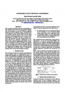
Fig. 1. Block diagram of the learning procedure.

are used for training the conversion function. As a further simplification the maximum voiced frequency was fixed at a constant value of 4 kHz. The conversion of the noise part is simply achieved by the use of two different correction filters (one for voiced frames and one for unvoiced frames). These correction filters, implemented as sixth-order all-pole filters, model the difference between the average noise spectra of the source and target speaker. The distinction between voiced and unvoiced frames appears to be necessary because the average characteristics of the noise part are very different in the two cases. The aim of the spectral conversion function is thus to transform the harmonic part of speech which is supposed to extend between 0 and 4 kHz (for voiced frames). The spectral envelope corresponding to the voiced part of speech is computed from the amplitudes of the harmonics by the discrete regularized cepstrum method using a warped frequency scale [3], [4]. The main steps of the envelope estimation procedure are as follows. 1) The amplitudes of the harmonics determined by the HNM analysis are expressed in the log domain. 2) The frequencies of the harmonics are converted to a Bark frequency scale using the analytical formulas reported in [50]. The obtained values are normalized in order to ensure that the upper limit of the band (4 kHz) corresponds to a value of on the normalized warped frequency axis. 3) The real cepstrum parameters that represent the envelope by (21) are obtained by minimizing the following least squares criterion in the log-spectral domain (22) is a penalty functional which only depends where on the shape of the envelope (and not on the constraints ). The form of is chosen so as to penalizes rapid variations [4]. The use of a penalty funcin the spectral envelope tional guarantees that the envelope obtained is well-behaved independent of any frequency constraints. The minimization of

(22) is equivalent to the solution of a linear system of equations [4]. The cepstral parameters obtained are similar to the usual MFCC’s [36] except for the fact that they are obtained from the minimization of a discrete set of frequency constraints. Such parameters were originally mentioned in [13] as discrete MFCC’s and are known to provide a better envelope fit (at the specified frequency points) than LPC-based methods [3]. The synthetic signals obtained by use of the envelope representation or by a direct synthesis from the HNM parameters are generally indistinguishable provided that the order of the cepstrum is greater than 16. For lower values of the cepstrum order, some smoothing of the envelope occurs, in particular in the high-frequency range. In order to maintain an accurate description of the characteristics of the spectral envelope, an order of was used throughout our voice conversion experiments. In the present study, the first cepstrum coefficient was omitted as a form of energy normalization. In practice, it was found that it is not advisable to include in the training parameters because it biases the classification achieved by the GMM. The spectral parameters are thus dimensional vectors which contain the discrete MFCC coefficients . C. Learning Procedure The complete learning procedure is depicted in Fig. 1. Note that for the training of the conversion function, the source and target signals are analyzed with a fixed 10 ms frame rate in order to allow time-alignment by the DTW algorithm. Recall that we only consider the time-intervals where the frames corresponding to both signals are marked as voiced. The optimization of the conversion function (rightmost block in Fig. 1) makes use of the time-aligned spectral envelopes (source) and (target) as well as the parameters of the GMM as estimated by the EM algorithm. Once a conversion function has been obtained, the process can be iterated by reestimating the time-alignment between the converted envelopes and the target envelopes. Iterative procedures have also been used in the literature for speakeradaptive training in continuous speech recognition [11]. These optional “incremental learning” steps are only intended to refine the time alignment path. The GMM estimation and the least squares (LS) optimization are of course always performed using the source envelopes (and not the converted envelopes). However, the LS optimization has to be entirely recomputed because the two sets of envelopes (source) and change with the time-alignment.

138

IEEE TRANSACTIONS ON SPEECH AND AUDIO PROCESSING, VOL. 6, NO. 2, MARCH 1998

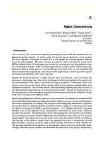
Fig. 2. Block diagram of the voice conversion system (not including the training of the spectral conversion function). tia : analysis time-instants, tis : synthesis time-instants.

D. Voice Conversion System

A. Objective Test

Once the spectral conversion function has been estimated, the voice transformation is performed as indicated in Fig. 2. The input of the system consists of speech signals sampled at 16 kHz. Note that for voice transformation, the HNM analysis is performed pitch-synchronously because this mode enables higher quality time-scale and pitch-scale modifications [46]. These modifications are PSOLA-like in that they mostly consist in recomputing the pitch-synchronous synthesis instants [31]. However, an important difference with the usual nonparametric TD-PSOLA (time domain pitch-synchronous overlap-add) processing is that the amplitude of the harmonics are computed explicitly using the converted spectral envelope (in the 0–4 kHz band and for voiced frames). The noise part is modified with two different fixed filters (so-called corrective filters) depending on whether the frame is voiced or not. In the present system, we do not consider the problem of matching the prosodic characteristics of both speakers. As a consequence, the prosodic modifications performed are merely intended to match the average fundamental frequency and articulation rhythm of both speakers. However, in (the rather artificial) case where the same sentence uttered by the two speakers is available, the HNM system can also be used to impose the pitch and time contours of the target speaker on the converted speech signals.

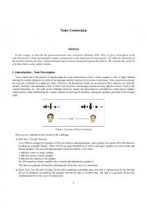
We studied the three types of conversion functions introduced in Section II (full, diagonal and VQ-type) as well as the original VQ-mapping approach of Abe et al. [1]. Fig. 3(b) presents the average rms log-spectral distortion as measured on the test corpus for these four methods as a function of the number of GMM components (or number of centroids in the case of VQ-mapping). The distortion was normalized by the initial average distortion between the two speakers. The rightmost points on Fig. 3(b) (128 label) correspond to the use of a 128 GMM component with one iteration of the incremental learning steps (by refinement of the time-alignment path). Fig. 3(a) shows the distortion between the converted and the source parameters (normalized as previously). The rms log-spectral distortion is computed using the warped frequency scale as

IV. RESULTS

AND

DISCUSSION

Our conversion methodology was tested on a conversion task between two male voices using a large amount of training data. The signal data base was provided by the Centre National d’Etudes des T´el´ecommunications (CNET) and consisted of short phonetic units uttered in context by the two speakers. This data base covers all the diphones of the French language and corresponds to approximately 20 000 training vectors (3.5 min of speech) once the unvoiced frames have been discarded. An independent corpus of about one minute of voiced speech signals was used to evaluate the performances of the proposed method. Note that the training data is made of approximately 1500 independent signal portions with an average duration of 150 ms. Each of these signal portions corresponding to the two speakers were aligned independently using a DTW procedure with relaxed endpoint constraints [36].

(23) where is the frequency warping function. In our case represent a normalized Hz to Bark frequency scale conversion. The obtained warped distortion is generally believed to be more perceptually relevant [36]. Note that the cepstral coeffiis omitted in (23) because it is not affected by the cient conversion function. The variations of the distortion curves of Fig. 3 may appear small, but it is necessary to keep in mind the following. 1) They pertain to time-aligned signal frames. In the present case, the initial average rms log-spectral distortion between the source and target envelopes is 8.2 dB. So that a 4 dB reduction of the distortion is indeed an appreciable difference. 2) The rms distortion is generally much lower than what we would expect by visual inspection of the envelopes: for example the rms log-spectral distortion between the dotted and the solid line envelopes of Fig. 4 is only 8.4 dB. The most striking feature of Fig. 3 is the fact that with the diagonal or the full conversion method the distortion between

STYLIANOU et al.: VOICE CONVERSION

139

(a)

Fig. 3. Average warped rms log-spectral distortion for the different types of conversion as a function of the number of GMM components. The 0 dB value refers to the initial distortion between the source and target envelopes. The label 1283 corresponds to the case where the time-alignment path is refined a posteriori (incremental learning). (a) Distortion between the converted and the source envelopes. (b) Distortion between the converted and the target envelopes. Dash-dot line: VQ-mapping. Dashed line: VQ-type conversion. Dotted line: diagonal conversion. Solid line: full conversion.

the source and the converted envelopes steadily increases with the number of GMM components [solid line and dotted line curves on Fig. 3(a)]. This is in total contrast with the behavior for VQ-based conversion, be it VQ-mapping (dashdot line) or VQ-type conversion (dotted line), where the distortion between the source and the converted envelopes starts from a very high value and decreases slowly as the number of centroids increases. In VQ-based conversion, the spectral transformation induces unwanted spectral distortion due to the discretization of the parameters space. The only way to improve this aspect in VQ-based method is by increasing the number of centroids. In this respect, the VQ-style conversion does not seem to perform any better than the standard VQmapping method. This last observation indicates that the limitations of VQ-based approaches can not be overcome by mere interpolation between the transformed centroids. Finally, the observed difference between the behaviors of the VQbased method and diagonal or full conversion method show the importance of the correction term in (5) that depends on . When looking at Fig. 3(b), it is clear that for a fixed number of GMM components, it is full conversion (solid line) that provides the largest spectral distortion reduction (between converted and target envelopes). However, we note that the performances of diagonal conversion using a component GMM is comparable to that of full conversion using a component GMM. This observation was verified for values up to 1024 (the highest value of that was tested in of the case of diagonal conversion). If we think in terms of the total number of parameters used for the conversion function, diagonal and full conversion do not appear to be very different. For diagonal conversion the total number of parameters is (or in our case since the dimension is set to

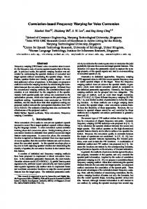
(b) Fig. 4. Envelope conversion for a 128 GMM (a) with diagonal conversion and (b) with full conversion. Dotted line: source envelope. Dashed line: converted envelope. Solid line: target envelope.

20), for full conversion it is . So that a component full conversion involves parameters compared to parameters for the diagonal conversion with an components GMM. It is expected, however, that full conversion should be much more effective than diagonal conversion in cases where the spectral vectors contain strongly correlated coefficients. The comparison of the distortions associated with the two rightmost points of each of the curves of Fig. 3(b) (labels 128 and 128 ) confirms the effictiveness of an additional incremental learning step. We observed that further iterations did not lead to significant improvements. However, it is important to consider that in our case the time-alignment errors are limited by the fact that DTW is only applied to short signal portions (150 ms on average) that have been manually end-pointed. Fig. 4(a) displays an example of envelope conversion with diagonal conversion and Fig 4(b) displays an example of envelope conversion with full type conversion. In this example, the warped rms log-spectral distortion is, respectively, 8.4 dB between the source (dotted line) and target (solid line) envelopes, 4.8 dB between the target envelope and the envelope converted by diagonal conversion [dashed line on Fig. 4(a)], and 2.2 dB between the target envelope and the envelope converted by full conversion [dashed line on Fig. 4(b)]. Note that the envelope is represented using a linear frequency scale. The influence of the warped frequency scale used for the cepstral parameters can be observed by noting that the spectral resolution of the envelope is best in the low-frequency range (below 1.5 kHz), which is particularly apparent for the source envelope (dotted line). Fig. 5 presents the frame rms log spectral distortion measured for one second of natural speech. As before, the 0 dB value refers to the initial average distortion between the source and target envelopes. In Fig. 5(a) which corresponds to the use

140

IEEE TRANSACTIONS ON SPEECH AND AUDIO PROCESSING, VOL. 6, NO. 2, MARCH 1998

RESULTS

TABLE I XAB TEST

FROM THE

(a)

Fig. 6. Preference score.

(b) Fig. 5. Normalized warped rms log-spectral distortion in dB for 100 consecutive frames of voiced speech. (a) Conversion by VQ-mapping (128 centroids). (b) Full conversion (128 GMM). Dash-dot line: distortion between source and target envelopes. Solid line: distortion between converted and target envelopes.

of VQ-mapping, it is observed that the reduction of the log spectral distortion by the conversion is very non uniform: The shapes of the distortion curves before (dash-dot line) and after (solid line) conversion are rather different. The VQ-mapping makes it possible to achieve an average distortion reduction of 3.9 dB but the distortion after conversion [solid line curve on Fig. 5(a)] frequently presents “spikes” where the distortion reduction is much lower. In contrast, Fig. 5(b) shows that the full conversion provides a more regular reduction of the log spectral distortion. With full conversion, the average distortion reduction is 4.9 dB and the reduction is almost always greater than 2 dB. B. Formal Listening Test The quality of the proposed conversion method was also assessed during formal listening tests on sentences uttered by the source and the target speakers. In order to evaluate only the spectral conversion aspect and thus demonstrating the efficiency of the proposed method for modifying spectral envelopes, the prosody of the source speaker has been altered to match as closely as possible the prosody of the target speaker. Prosodic modifications were carried out using HNM. Then, the conversion function was applied on the modified speech, using full conversion for a 16 GMM and a 64 GMM. The evaluation has been carried out using three continuously uttered sentences of about 4 s duration each. Three kinds of listening tests have been designed; XAB test, preference test and opinion test. Twenty listeners participated in each of these experiments. 1) XAB Test: To evaluate the accuracy of the conversion, a set of triads were presented to the listeners using the XAB method. X was either the prosodic only modified speech, the converted speech by using 16 GMM or the converted

Fig. 7. Opinion test.

speech by using 64 GMM (always using the full conversion approach). A and B were either the target or the source speaker. Speakers A and B uttered the same sentence which, in general, was different from the sentence uttered by X. Subjects were asked to select either A or B as being most similar to X. Table I summarizes the results from this test giving the percentage of correct answers. A correct answer means that the converted/modified speaker was recognized as the target speaker. This table shows that when we modified only the prosody of the source speaker the identity of the speaker was not perceived as changed. However, when we applied the conversion function using 16 GMM the percentage of correct answers increase notably. This continues to increase when the number of components is increased to 64. The last column of the Table I refers to the score of the correct answers using 64 GMM and when X, A and B utter the same sentence. The task of the listeners was easier in this case and this is reflected in the higher score. 2) Preference Test: To compare the quality of the converted signal using different numbers of GMM components a preference test was designed. In this test, pairs of converted speech with 16 and 64 GMM components were presented to the subjects. The listeners were asked to give their preference for each pair of converted speech. Listeners preferences are

STYLIANOU et al.: VOICE CONVERSION

shown in Fig. 6. The overall quality of the converted signals was considered as “rather natural” although some of the listeners reported a muffling effect when the number of GMM components was small. 3) Opinion Test: In an effort to evaluate the overall performance of the proposed method, an opinion test was designed. Pairs of speech signals, including all possible combinations of original speaker, target speaker, “prosodic modified” speaker and converted speaker using 16 and 64 GMM components, were presented to the listeners. Different sentences were used to make these pairs. Listeners were asked to rate the similarity of each pair of speakers on a scale with ten values between zero for “identitical” and nine for “very different.” Fig. 7 presents the results from this test. The symbols used in this figure stand for the distances: “TT,” target-target, “SS,” source-source, “M2,” converted speaker using 64 GMM components-target, “M1,” converted speaker using 16 GMM components-target, “PT,” prosodic modified speaker-target, and “ST,” source-target. For each of the distances the median value is given (noted by “x”) as well as the variation of the decisions using as estimator the mean absolute deviation rather than the standard deviation. This figure clearly shows the efficiency of the proposed method and confirm the results of the first test. Modifying only the prosody of the source speaker, perceived speaker identity does not change markedly. The distance “PT” is very close to that of “ST.” However, applying the conversion function after the prosodic modifications, the converted speech approaches the score which is obtained when same speakers are compared. Also, clearly when the number of GMM components was increased the results were much better (at the cost of using more data during the learning step). Further studies are currently being conducted to measure the conversion effect due to various choices of spectral parameters.

V. CONCLUSION The method proposed for the conversion of the spectral envelopes of speech is more robust and efficient than methods based on VQ. This improvement is a consequence of the use of a continuous probabilistic model of the source envelopes. It also appears that the design of the conversion function plays an important part. The most efficient conversion functions (diagonal and full types) are those that take into account the variability of the source spectral envelopes that are associated with each mixture component. The use of diagonal matrices for the GMM and for the conversion function does not degrade the conversion performances, given that a sufficient number of mixture components are used. This last result would probably not hold for spectral parameters that are more correlated than cepstrum coefficients. The efficiency of the incremental learning procedures points out the difficulty of determining a reliable time-alignment path by dynamic time warping. Objective tests and formal listening tests confirmed the effectiveness of the proposed transform function, showing that high-quality voice conversion can be obtained by combining the proposed continuous probabilistic transform with the HNM for speech.

141

ACKNOWLEDGMENT The authors wish to thank anonymous reviewers as well as J. Schroeter for their critical review and their help in improving our paper. The authors are indebted to J. Laroche for his encouragement and his continuous support during this work.

REFERENCES [1] M. Abe, S. Nakamura, K. Shikano, and H. Kuwabara, “Voice conversion through vector quantization,” in Proc. IEEE Int. Conf. Acoustics, Speech, Signal Processing, 1988, pp. 655–658. , “Voice conversion through vector quantization,” J. Acoust. Soc. [2] Jpn., vol. E-11, pp. 71–77, Mar. 1990. [3] O. Capp´e, J. Laroche, and E. Moulines, “Regularized estimation of cepstrum envelope from discrete frequency points,” in Proc. IEEE ASSP Workshop on Applications of Signal Processing to Audio and Acoustics, Mononk, NY, Oct. 1995. [4] O. Capp´e and E. Moulines, “Regularization techniques for discrete cepstrum estimation,” IEEE Signal Processing Lett., vol. 3, pp. 100–102, Apr. 1996. [5] C. Chatfield and A. J. Collins, Introduction to Multivariate Analysis. London, U.K.: Chapman & Hall, 1980. [6] A. P. Dempster, N. M. Laird, and D. B. Rubin, “Maximum likelihood from incomplete data via the EM algorithm,” J. R. Stat. Soc. B, vol. 39, pp. 1–22 and 22–38, 1977. [7] G. Doddington, “Speaker recognition—Identifying people by their voices,” in Proc. IEEE, vol. 73, pp. 1651–1664, 1985. [8] R. O. Duda and P. E. Hart, Pattern Classification and Scene Analysis. New York: Wiley, 1973. [9] W. Endres, W. Bambach, and G. Fl¨osser, “Voice spectrograms as a function of age, voice disguise, and voice imitation,” J. Acoust. Soc. Amer., vol. 49, pp. 1842–1848, 1971. [10] B. S. Everitt and D. J. Hand, Finite Mixture Distributions. London, U.K.: Chapman & Hall, 1981. [11] M.-W. Feng, F. Kubala, R. Schwartz, and J. Makhoul, “Iterative normalization for speaker-adaptive training in continuous speech recognition,” in Proc. IEEE ICASSP-89, pp. 612–615. [12] S. Furui, “Research on individuality features in speech waves and automatic speaker recognition techniques,” Speech Commun., vol. 5, pp. 183–197, 1986. [13] T. Galas and X. Rodet, “Generalized functional approximation for source-filter system modeling,” in Proc. Eurospeech, Genoa, Italy, 1991, pp. 1085–1088. [14] H. Gish and M. Schmidt, “Text-independent speaker identification,” IEEE Signal Processing Mag., vol. 11, pp. 18–32, Oct. 1994. [15] U. G. Goldstein, “Speaker-identifying features based on formant tracks,” J. Acoust. Soc. Amer., vol. 59, pp. 176–182, 1975. [16] Y. Gu and J. S. Mason, “Speaker normalization via a linear transformation on a perceptual feature space and its benefits in ASR adaptation,” in Proc. Europ. Conf. Speech Communication and Technology, 1989, pp. 258–261. [17] H. Hollien, The Acoustics of Crime—The New Science of Forensic Phonetics. New York: Plenum, 1990. [18] K. Itoh and S. Saito, “Effects of acoustical feature parameters on perceptual speaker identity,” Rev. Electr. Commun. Labs., vol. 36, pp. 135–141, 1988. [19] N. Iwahashi and Y. Sagisaka, “Speech spectrum transformation by speaker interpolation,” in Proc. IEEE Int. Conf. Acoustics, Speech, Signal Processing, 1994. [20] N. Iwahashi and Y. Sagisaka, “Speech spectrum conversion based on speaker interpolation and multi-functional representation with weighting by radial basis function networks,” Speech Commun., vol. 16, pp. 139–151, Feb. 1995. [21] C. C. Johnson, H. Hollien, and J. W. Hicks, “Speaker identification utilizing selected temporal speech features,” J. Phonet., vol. 12, pp. 319–326, 1984. [22] S. M. Kay, Fundamentals of Statistical Signal Processing: Estimation Theory. Englewood Cliffs, NJ: Prentice-Hall, 1993. [23] H. Kuwabara and Y. Sagisaka, “Acoustic characteristics of speaker individuality: Control and conversion,” vol. 16, pp. 165–173, Feb. 1995. [24] J. Laroche, Y. Stylianou, and E. Moulines, “HNS: Speech modification based on a harmonic noise model,” in Proc. IEEE ICASSP-93, Minneapolis, MN, Apr. 1993. [25] C. L. Lawson and R. J. Hanson, Solving Least-Squares Problems. Englewood Cliffs, NJ: Prentice-Hall, 1974.

+

142

IEEE TRANSACTIONS ON SPEECH AND AUDIO PROCESSING, VOL. 6, NO. 2, MARCH 1998

[26] Y. Linde, A. Buzo, and R. M. Gray, “An algorithm for vector quantizer design,” IEEE Trans. Commun., vol. 28, 1980. [27] N. Merhav and C.-H. Lee, “On the asymptotic statistical behavior of empirical cepstral coefficients,” IEEE Trans. Acoust., Speech, Signal Processing, vol. 41, pp. 1990–1993, 1993. [28] H. Mizuno and M. Abe, “Voice conversion based on piecewise linear conversion rule of formant frequency and spectrum tilt,” in Proc. IEEE Int. Conf. Acoustics, Speech, Signal Processing, 1994. , “Voice conversion algorithm based on piecewise linear conver[29] sion rule of formant frequency and spectrum tilt,” Speech Commun., vol. 16, pp. 153–164, Feb. 1995. [30] C. Mokbel and G. Chollet, “Speech recognition in adverse environments: Speech enhancement and spectral transformations,” in Proc. IEEE ICASSP-91, pp. 925–928. [31] E. Moulines and J. Laroche, “Techniques for pitch-scale and timescale transformation of speech, Part I: Nonparametric methods,” Speech Commun., vol. 16, Feb. 1995. [32] E. Moulines and Y. Sagisaka, Eds., Voice Conversion: State of the Art and Perspectives (Special Issue of Speech Communication). Amsterdam, The Netherlands: Elsevier, vol. 16, Feb. 1995. [33] L. Neumeyer and M. Weintraub, “Probabilistic optimum filtering for robust speech recognition,” in Proc. IEEE Int. Conf. Acoustics, Speech, Signal Processing, Adelaide, Australia, 1994, pp. 417–420. [34] W. H. Press, S. A. Teukolsky, W. T. Vettering, and B. P. Flannery, Numerical Recipes in C, 2nd Ed. Cambridge, U.K.: Cambridge Univ. Press, 1994. [35] T. F. Quatieri, C. R. Jankowski, Jr., and D. A. Reynolds, “Energy onset times for speaker identification,” IEEE Signal Processing Lett., vol. 1, Nov. 1994. [36] L. R. Rabiner and B.-H. Juang, Fundamentals of Speech Recognition. Englewood Cliffs, NJ: Prentice-Hall, 1993. [37] R. A. Redner and H. F. Walker, “Mixture densities, maximum likelihood and the EM algorithm,” SIAM Rev., vol. 26, pp. 195–239, Apr. 1984. [38] D. A. Reynolds, “A Gaussian mixture modeling approach to textindependent speaker identification,” Ph.D. dissertation, Georgia Inst. Technol., Atlanta, Aug. 1992. [39] D. A. Reynolds and R. C. Rose, “Robust text-independent speaker identification using Gaussian mixture speaker models,” IEEE Trans. Speech Audio Processing, vol. 3, pp. 72–83, Jan. 1995. [40] R. C. Rose and D. A. Reynolds, “Text independent speaker identification using automatic acoustic segmentation,” in Proc. IEEE Int. Conf. Acoustics, Speech, Signal Processing, 1990, pp. 293–296. [41] A. E. Rosenberg and F. K. Soong, “Recent research in automatic speaker recognition,” Advances in Speech Signal Processing, S. Furui and M. Sondhi, Eds. New York: Marcel Dekker, 1991, pp. 701–738. [42] M. R. Sambur, “Selection of acoustic features for speaker identification,” IEEE Trans. Acoust., Speech, Signal Processing, vol. ASSP-23, pp. 176–182, 1975. [43] K. Shikano, K. Lee, and R. Reddy, “Speaker adaptation through vector quantization,” in Proc. IEEE Int. Conf. Acoustics, Speech, Signal Processing, 1986, pp. 2643–2646. [44] Y. Stylianou, “Harmonic plus noise models for speech, combined with statistical methods, for speech and speaker modification,” Ph.D. dissertation, Ecole Nat. Sup`erieure T´el´ecommun., France, Jan. 1996. [45] , “A pitch and maximum voiced frequency estimation technique adapted to harmonic models of speech,” in Proc. IEEE Nordic Signal Processing Symp., Helsinki, Finland, Sept. 1996. [46] Y. Stylianou, J. Laroche, and E. Moulines, “High-quality speech modification based on a harmonic noise model,” in Proc. EUROSPEECH, Madrid, Spain, 1995. [47] B. L. Tseng, F. K. Soong, and A. E. Rosenberg, “Continuous probabilistic acoustic map for speaker recognition,” in Proc. IEEE Int. Conf. Acoustics, Speech, Signal Processing, 1992, pp. II-161–II-164. [48] H. Valbret, E. Moulines, and J. P. Tubach, “Voice transformation using PSOLA techniques,” Speech Commun., vol. 11, pp. 175–187, June 1992. [49] C. F. J. Wu, “On the convergence properties of the EM algorithm,” Ann. Stat., vol. 11, pp. 95–103, 1983. [50] E. Zwicker and E. Terhardt, “Analytical expressions for critical-band rate and critical bandwidth as a function of frequency,” J. Acoust. Soc. Amer., vol. 68, pp. 1523–1525, 1980.

+

Yannis Stylianou (S’92–M’95) was born in Kounavous, Crete, Greece, on November 29, 1966. He received the Dipl. degree in electrical engineering from the National Technical University of Athens, Greece, in 1991, and the M.Sc. and Ph.D. degrees in signal processing from the Ecole Nationale Sup´erieure des T´el´ecommunications, Paris, France, in 1992 and 1996, respectively. In September 1995, he joined the Signal Department at Ecole Sup´erieure des Ingenieurs en Electronique et Electrotechnique, Paris, where he worked as an Assistant Professor of electrical engineering. From August 1996 until July 1997, he was with AT&T Laboratories–Research, Murray Hill, NJ, as a consultant in text-to-speech synthesis. In August 1997, he joined AT&T Labs–Research as a Senior Technical Staff Member. His current research focuses on speech synthesis, statistical signal processing, speech transformation, and low bit rate speech coding. Dr. Stylianou is a member of the Technical Chamber of Greece.

Olivier Capp´e (S’92–M’93) was born in Villeurbanne, France, in 1968. He received the M.Sc. degree in electrical engineering from the Ecole Sup´erieure d’Electricit´e, Paris, France, in 1990, and the Ph.D. degree in signal processing from the Ecole Nationale Sup´erieure des T´el´ecommunications (ENST), Paris, in 1993. His Ph.D. dissertation dealt with noise reduction for degraded audio recordings. From 1995 to 1996, he was with the Centre National d’Etudes des T´el´ecommunications (CNET), where he worked on speech and speaker recognition. He is now with the Centre National de la Recherche Scientifique (CNRS) at ENST-URA 820. His current research interests are in statistical modeling applied to various signal processing problems including noise reduction, speech processing, and blind identification. Dr. Capp´e received the IEEE Signal Processing Society’s Young Author Best Paper Award in 1995.

Eric Moulines (M’91) was born in Bordeaux, France, in 1963. He received the M.S. degree from Ecole Polytechnique in 1984, and the Ph.D. degree in signal processing from Ecole Nationale Sup´erieure des T´el´ecommunications (ENST) in 1990. From 1986 until 1990, he was a Member of the Technical Staff at CNET, working on signal processing applied to low bit rate speech coding and text-to-speech synthesis. Since 1990, he has been with ENST, where he is currently a Professor. His teaching and research interests include statistical signal processing and speech processing. Currently, he is engaged in research in various aspects of statistical signal processing including, among others, single and multichannel ARMA filtering and modeling, blind signal processing for digital communications, characterization and estimation of point processes with application to high bit rate data traffic modeling, low bit rate speech coding, and speech transformation. Dr. Moulines is an Associate Editor of Speech Communication and the IEEE TRANSACTIONS ON SIGNAL PROCESSING. He is a member of the IEEE committees on Speech and Statistical and Array Processing.