Continuous quantum measurement with independent detector cross ...

Continuous quantum measurement with independent detector cross-correlations Andrew N. Jordan and Markus B¨ uttiker

arXiv:cond-mat/0505044v1 [cond-mat.mes-hall] 2 May 2005

Département de Physique Théorique, Université de Genève, CH-1211 Genève 4, Switzerland (Dated: May 2, 2005) We investigate the advantages of using two independent, linear detectors for continuous quantum measurement. For single-shot quantum measurement, the measurement is maximally efficient if the detectors are twins. For weak continuous measurement, cross-correlations allow a violation of the Korotkov-Averin bound for the detector’s signal-to-noise ratio. A vanishing noise background provides a nontrivial test of ideal independent quantum detectors. We further investigate the correlations of non-commuting operators, and consider possible deviations from the independent detector model for mesoscopic conductors coupled by the screened Coulomb interaction. PACS numbers: 03.65.Ta, 73.23.-b, 03.65.Yz

There has recently been intensive research, both experimental and theoretical, into the development of quantum detectors in the solid state. Mesoscopic structures, such as the quantum point contact, single electron transistor, and SQUID have been used for fast qubit read-out. Contrary to the historical assumption that the quantum measurement occurs instantaneously, in the modern theory of quantum detectors the continuous nature of the measurement process is essential to the understanding and optimization of how quantum information is collected. The ultimate goal for quantum computation is the development of “single-shot” detectors, where in one run the qubit’s state is unambiguously determined. An important figure of merit is the detector’s efficiency, defined as the product of the time taken to measure the state of the qubit, with the measurement induced dephasing rate. This efficiency is minimized for detectors that do not lose information about the quantum state as the measurement is being performed. Single-shot detectors are difficult to realize because of the fast time resolution required. Another approach is that of weak measurement, where detector backaction renders the state of the qubit invisible in the average output of the detector, but quantum coherent oscillations are uncovered in the spectral density of the detector. These measurements are easier to preform because both detector and qubit averaging are permitted, and the experiments only require a bandwidth resolution of the qubit energy splitting. One important result in weak measurement theory is the Korotkov-Averin bound. It states that as the weak measurement is taking place, the detector backaction quickly destroys the quantum oscillations, so the maximum detector signal-to-noise ratio is fundamentally limited at 4. This result was derived in Refs. [1], confirmed in Refs. [2], generalized in Refs. [3], and measured in Ref. [4]. In this Letter, the theoretical advantages of considering the cross-correlated output of independent quantum detectors are investigated. It is clear that cross-correlations bestow an experimental advantage [5] in quantum measurement, because the procedure filters out any noise not

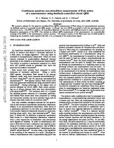
shared by the two detectors. Thus, extraneous noise produced by sources such as charge traps in one detector will be removed. This technique is also used in quantum noise measurements for this same advantage [6]. We demonstrate that although the two detectors cannot improve the efficency of the detection process, the cross-correlated output can violate the Korotkov-Averin bound. As a solid-state implementation of the results derived, Fig. 1 depicts two quantum point contacts capacitively coupled to the same double quantum-dot representing a charge qubit. It should be stressed that such structures have already been fabricated [7]. Detector assumptions and linear response.– We employ the linear response approach to quantum measurement because of its elegant simplicity, and general applicability to a wide range of detectors [1, 8, 9]. The quantum operator to be measured is σz . The Hamiltonian is H = −(ǫ σz +∆σx )/2+H1 +H2 +Q1 σz /2+Q2 σz /2, (1) where Q1,2 are the bare input variables of detector 1 and 2, and H1,2 are their Hamiltonians, and I1,2 are the bare output variables of the detectors. The small coupling constants are incorporated into the definition of Q1,2 . We assume that the detector is much faster than all qubit

Ci

11111 00000 00000 11111 C1 C2 00000 Q1 Qq −Qq V1 11111 00000 11111 00000 11111 00000 11111

1111 0000 0000 1111 0000 1111 Q2 V2 0000 1111 0000 1111 0000 1111

FIG. 1: Cross-correlated quantum measurement set-up: Two quantum point contacts are measuring the same double quantum dot qubit. As the quantum measurement is taking place, the current outputs of both detectors can be averaged or crosscorrelated with each other.

2 time scales, so the relevant detector correlation functions are the stationary zero frequency correlators: (i)

hIi (t + τ )Ij (t)i = SI δij δ(τ ),

(2a)

hQi (t + τ )Qj (t)i =

(2b)

hQi (t + τ )Ij (t)i =

(i) SQ δij δ(τ ),

(i) (ReSQI (i)

+

(i) i ImSQI )δij δ(τ ),

(2c)

(i)

hIi (t + τ )Qj (t)i = (ReSQI − i ImSQI )δij δ(τ ). (2d) where the time delta functions have a small shift δ(τ −0), reflecting the finite response time of the detector. Linear response theory tells us that the response coefficients λ1,2 (i) are given by λi = −2 ImSQI /~, so the output of the detectors (with the average subtracted) is Oi = Ii +λi σz /2. As the detector is turned on, it ideally collects information about the operator σz while destroying information about σx,y . The measurement is complete when the integrated difference in qubit signal exceeds the detector noise, so the state of the qubit may be determined. In the simplest case of ∆ = 0, the standard expressions for the dephasing rate Γ and measurement time TM are [10] Γ = SQ /(2~2 ),

TM = 4SI /λ2 .

(3)

Let us next observe ~2 λ2 = 4(ImSQI )2 ≤ 4|SQI |2 ≤ 4SQ SI ,

(4)

where we have used the Cauchy-Schwartz inequality. For a lone detector the above relations imply ΓTM ≥ 1/2, where equality is reached for quantum limited detectors. The two conditions needed to reach the “Heisenberg efficiency” are, (a) ReSQI = 0,

(b) |SQI |2 = SQ SI .

(5)

In the context of mesoscopic scattering detectors, condition (b) is related to the energy dependence of the transmission of the scatterer, while (a) is related to the symmetry of the scatterer [1]. Pilgram and one of the authors derived Eqs. (5) for arbitrary detectors described by scattering matrices [8]. Clerk, Girvin, and Stone interpreted these conditions as no lost information either through (a) phase or (b) energy averaging [9]. Can we do better with two detectors?– By adding an additional detector to the qubit, the signals may be averaged, O = (O1 + O2 )/2, so the measurement time may be reduced. On the other hand, the new detector dephases the qubit more quickly. For statistically independent detectors, the measurement-induced dephasing rate is simply the sum of the individual dephasing rates, so the two-detector efficiency is ΓTM =

(1) 2(SI

+

(2) (1) SI )(SQ

+

(2) SQ )/~2 (λ1

2

+ λ2 ) ≥ 1/2, (6) where equality is reached for twin detectors that are themselves quantum limited. This condition may also be

interpreted as no lost information between the two detectors. Rather than average the signals, we could instead cross-correlate them. However, this also brings no advantage because the new signal obtained by multiplying the output from the two detectors, O1 (t1 )O2 (t2 ), has its own noise. If we could average over many trials the noise could be eliminated, but for single-shot measurement the efficiency is still intrinsically limited. Violation of the Korotkov-Averin bound.– But consider next Korotkov and Averin’s bound on the signalto-noise ratio for a weakly measured qubit [1]. It states that the ratio of the measured qubit signal to detector noise, R, is fundamentally limited by 4. This bound can be overcome with quantum nondemolition measurements by increasing the signal [11]. In this Letter, we are concerned with reducing the noise. To see how this bound emerges, we briefly derive this inequality for one detector. The Hamiltonian is given by Eq. (1) with Q2 = 0. The time averaged output of the detector is RT hOi = (λ/2)(1/T ) 0 dthσz (t)i. For a weakly measured qubit, the statistical average over σz is taken with respect to the stationary, mixed, density matrix of the qubit, ρ = (1/2)11, and therefore the qubit makes no contribution to the average output current. The detector’s spectral density is S(ω) = SI + (λ2 /4)Szz (ω), where Z ∞ dt cos(ωt)hσi (0)σj (t)i. (7) Sij (ω) = 2 0

The qubit dynamics may be found by expanding the evolution operator to second order in the coupling constant, and averaging over the δ-correlated Q fluctuations to obtain equations of motion, with dephasing rate Γ. For the special case of ǫ = 0, the noise spectrum in the vicinity of ω = ∆/~ ≡ Ω is [1] S(ω) = SI +

Ω2 λ2 Γ . 2 (ω 2 − Ω2 )2 + ω 2 Γ2

(8)

At the qubit frequency, ω = Ω, the signal has a maximum of Smax = λ2 /(2Γ) = ~2 λ2 /SQ . We use again the linear response relation (4) to bound the signal-to-noise ratio of the detector as R = Smax /SI ≤ 4.

(9)

This is the Korotkov-Averin bound. Consider now the cross-correlation of the outputs from two independent detectors, both measuring the same qubit operator σz . The qubit dynamics is the same, except that Γ = Γ1 + Γ2 . The spectral density of the cross-correlation S1,2 (ω) contains four terms, Z ∞ S1,2 (ω) = dt cos(ωt)[2hI1 (0)I2 (t)i + λ1 hσz (0)I2 (t)i 0

+ λ2 hI1 (0)σz (t)i + (λ1 λ2 /2)hσz (0)σz (t)i]. (10) According to Eq. (2a) the bare detector noise of the two detectors are uncorrelated, the qubit dynamics is uncorrelated with the bare detector noise, so only the qubit

3

(1, 0, 0)

0.5

(b)

0

-0.40

(0, 0, 0)

(c)

0.5

1

ω/∆

+αλ2 hI1 (0)Q1 (t)i + α2 λ1 λ2 hQ1 (0)Q2 (t)i].

(12)

The first and last term vanish for independent detectors, leaving the middle two terms. These middle terms may be interpreted as a fluctuation in one detector causing a response in the other detector, which is then correlated back with the original bare detector variable in the signal multiplication. Using the correlators Eq. (2c,2d), we find (1)

δS1,2 = αλ1 ReSQI + αλ2 ReSQI ,

(13)

where we have substituted the response coefficient for the imaginary part of the Q-I correlator, which causes the imaginary part of the additional cross-correlated signal to vanish. An interesting aspect of the above equation is that if the detectors are both quantum limited, we saw in Eq. (5a) that one condition was that the real part of the Q-I correlator should vanish. Eq. (13) provides a simple experimental test to check this condition: background cross-correlations should vanish. If this is true, then the direct coupling between detectors does not give any noise pedestal to overcome for weak measurement. Weak measurement of non-commuting observables.— Once we have two detectors involved, there is no reason why they both have to measure the same observable (or

Szz 00

1

ω/∆

2

3

00

2

3

ε = .5 ∆ 1∆ 2∆

(d)

(2)

where equality is reached for SQ = SQ . For twin detectors, (11) is half of the single detector signal, because of the doubled dephasing rate [12]. We have successfully removed the background noise, and can now see the naked destruction of the qubit. The signal-to-noise ratio R is divergent, violating the Korotkov-Averin bound. Why did cross-correlations help here, but not in the quantum efficency? The reason is that the spectral density, in contrast to the measurement efficiency, is not protected by the uncertainty principle, so there is no fundamental limitation on its measurement. Detecting the detector.— Although the above result is very appealing, one might worry that it can be spoiled by some weak direct coupling between the detectors. We now take this into account by introducing another term in the Hamiltonian, H1,2 = αQ1 Q2 , where α is a relative coupling constant between the two detectors. The additional contribution to the zero-frequency cross-correlator, R δS1,2 = dthδO1 (0)δO2 (t)i, consists of four terms, Z δS1,2 = dt[hI1 (0)I2 (t)i + αλ1 hQ2 (0)I2 (t)i

(2)

x y

Sxx

(1)

0.4

(a) z

Szx

signal (7) contributes to the correlation function (10). The remaining question is the detector configuration that maximizes the signal. The maximum signal at ω = Ω is Smax = λ1 λ2 /[2(Γ1 + Γ2 )], and we may use the relations (4) to bound the cross-correlated signal in relation to the noise of the individual detectors as q (1) (2) (11) Smax ≤ 2 SI SI ,

1

ω/∆

2

3

FIG. 2: (color online). (a) Time domain destruction of the quantum state by the weak measurement process for ǫ = ∆. The elapsed time is parameterized by color, and (x,y,z) denote coordinates on the Bloch sphere. (b) The measured crosscorrelator Szx (ω) changes sign from positive at low frequency (describing incoherent relaxation) to negative at the qubit oscillation frequency (describing out of phase, coherent oscillations). (c,d) The correlators Sxx , Szz have both a peak at zero frequency and at qubit oscillation frequency. We take Γ = Γx = Γz = .07∆/~. Sij are plotted in units of Γ−1 .

one that commutes with it). We now consider an experiment where one detector measures σz and the other measures σx , and the outputs are cross-correlated. The measured spectrum is S1,2 (ω) = (λ1 λ2 /4)Szx (ω). This experiment could be implemented with a split Cooperpair box [13], where a SQUID is weakly measuring the persistent current, and a quantum point contact is weakly measuring the electrical charge. In standard measurement theory, the question of a simultaneous measurement of non-commuting observables cannot even be posed. The coupling part of the Hamiltonian is altered to be Hc = (1/2)Q1 σz + (1/2)Q2 σx . We P parameterize any traceless qubit operator as σ(t) = i xi (t)σxi , and the density matrix ρ = (1/2)11 + σ(t), so (x, y, z) also represent coordinates on the Block sphere. Defining (2) (1) Γz = SQ /(2~2 ), Γx = SQ /(2~2 ), the equations of motion for xi , averaged over the white noise of Q1 and Q2 , are      x˙ x −Γz −ǫ/~ 0 y˙  =  ǫ/~ −Γx − Γz −∆/~ y  . (14) z˙ z 0 ∆/~ −Γx Diagonalization of the transition matrix in the case Γx = 0 gives the usual expressions for the dephasing and relaxation rates. This set-up is always far away from the Heisenberg efficiency because one detector is destroying the signal the other is trying to measure. However, this situation has interesting behavior in the weak measurement case. The cross-correlation S1,2 (Ω) attains its maximum signal at the symmetric point ǫ = ∆, Γx = Γz = Γ,

4 √ so the qubit frequency is Ω = 2∆/~. The master equation may be solved in the weak dephasing limit, giving the correlation (for positive frequencies) Sxz (ω) = Szx (ω) =

3Γ Γ − 2 . (15) Γ2 + ω 2 9Γ + 4(ω − Ω)2

The first term has a peak at zero frequency, while the second term has a peak at ω = Ω, with width 3Γ/2, and signal −1/3Γ. Bounding this signal in relation to the noise in the individual twin detectors gives |S1,2 (Ω)| ≤ (2/3)SI . The interesting feature of this correlator is that it changes sign as a function of frequency. The low frequency part describes the incoherent relaxation to the stationary state, while the high frequency part describes the out of phase, coherent oscillations of the z and x degrees of freedom. The measured correlator Szx , as well as Sxx , Szz are plotted as a function of frequency in Fig.2(b,c,d) for different values of ǫ. These correlators all describe different aspects of the time domain destruction of the quantum state by the weak measurement, visualized in Fig.2a. We note that the cross-correlator changes sign for ǫ = −∆. Implementation.– We now consider two quantum point contacts, measuring a double quantum dot qubit. The point contact perfectly obeys conditions (5) and is thus an ideal detector [1, 8, 9]. The bare input detector variable Q is identified with the electrical charge in the point contact, while the bare output variable I is identified with the shot noise. The conductance of the QPC is sensitive to the electron’s position on the double dot. A measurement of the quantum state occurs when the integrated current difference exceeds the shot noise power. In the geometry shown in Fig. 1, one detector measures σz , while the other detector measures −σz , so the qubit signal will be anti-correlated. The charges on the two detectors are not independent, but rather must be the opposite of each other to have charge neutrality in the system. This electrical screening generates correlations between the potentials of the two quantum point contacts, increasing the dephasing rate, hurting the efficiency, and producing some background noise for the cross-correlator. This situation is markedly in contract with the single detector case [8], where screening simply renormalized the coupling constant. However, in realistic detectors there will always be other gates to control the quantum double dot, creating a larger capacitance matrix than the minimal one shown in Fig. 1. In this extended geometry, a charge fluctuation in one detector will be screened by the surrounding metallic gates, not by the other detector, justifying the independent detector model. We mention that in the experiment already done by Buehler et al. [5], the detectors seem to be completely independent. Conclusions.– We considered the advantages that two independent quantum detectors measuring the same qubit can bring to the quantum measurement problem.

The Heisenberg efficiency could be reached with quantum limited twin detectors. The asymmetry of the detector, related to phase information in the case of mesoscopic scattering detectors, could be measured with lowfrequency cross-correlations, and thus provides a nontrivial experimental test for quantum efficiency. For weak continuous measurement, the cross-correlated signal removes the noise pedestal, and allows a violation of the Korotkov-Averin bound on the signal-to-noise ratio. The cross-correlation of non-commuting operators were also investigated, which showed a cross-over from positive to negative correlation as a function of frequency. Although we have focused on mesoscopic qubits, this technique easily extends to other systems where similar bounds have been derived, such as single spins and nano-mechanical oscillators [14]. We thank A. N. Korotkov and D. V. Averin for correspondence and suggestions. This work was supported by the SNF and MaNEP. [1] A. N. Korotkov and D. V. Averin, Phys. Rev. B 64, 165310 (2001); A. N. Korotkov, Phys. Rev. B 63, 085312 (2001); D. V. Averin, in Exploring the Quantum/Classical Frontier, edited by J. R. Friedman and S. Han (Nova Science Publishes, New York, 2003), p. 447; cond-mat/0004364. [2] H. S. Goan and G. J. Milburn, Phys. Rev. B 64, 235307 (2001); R. Ruskov and A. N. Korotkov, Phys. Rev. B 67, 075303 (2003); A. Shnirman, D. Mozyrsky, and I. Martin, Europhys. Lett. 67, 840 (2004). [3] W. Mao, D. V. Averin, R. Ruskov, and A. N. Korotkov, Phys. Rev. Lett. 93, 056803 (2004); W. Mao, D. V. Averin, F. Plastina, and R. Fazio, Phys. Rev. B 71, 085320 (2005). [4] E. Il’ichev et al., Phys. Rev. Lett. 91, 097906 (2003). [5] T. M. Buehler et al., App. Phys. Lett. 82, 577 (2002). [6] A. Kumar et al., Phys. Rev. Lett. 76, 2778 (1996). [7] J. M. Elzerman et al., Phys. Rev. B 67, 161308(R) (2003). [8] S. Pilgram and M. B¨ uttiker, Phys. Rev. Lett. 89, 200401 (2002). [9] A. A. Clerk, S. M. Girvin, and A. D. Stone, Phys. Rev. B 67, 165324 (2003). [10] Y. Makhlin, G. Sch¨ on, and A. Shnirman, Rev. Mod. Phys. 73, 357 (2001). [11] D. V. Averin, Phys. Rev. Lett. 88, 207901 (2002); A. N. Jordan and M. B¨ uttiker, Phys. Rev. B 71, 125333 (2005). [12] The response functions may be quite different, so the (2) (1) cross-correlated signal Smax ≤ 2SI λ1 /λ2 = 2SI λ2 /λ1 may be much larger than the noise in one detector, provided it is much smaller than the noise in the other detector. [13] D. Vion et al., Science 296, 886 (2002); Y. Nakamura, Yu. A. Pashkin, and J. S. Tsai, Nature 398, 786 (1999); V. Bouchiat et al., Phys. Scr. T76, 165 (1998); M. B¨ uttiker, Phys. Rev. B 36, 3548 (1987); [14] L. N. Bulaevskii and G. Ortiz, Phys. Rev. Lett. 90, 040401 (2003); A. A. Clerk, Phys. Rev. B 70, 245306 (2004).