Continuous Time Bayesian Network Reasoning and Learning Engine

Journal of Machine Learning Research 11 (2010) 1137-1140

Submitted 10/09; Revised 1/10; Published 3/10

Continuous Time Bayesian Network Reasoning and Learning Engine Christian R. Shelton Yu Fan William Lam Joon Lee Jing Xu

CSHELTON @ CS . UCR . EDU YFAN @ CS . UCR . EDU WLAM @ CS . UCR . EDU JLEE 133@ CS . UCR . EDU JINGXU @ CS . UCR . EDU

Department of Computer Science and Engineering University of California Riverside, CA 92521, USA

Editor: Soeren Sonnenburg

Abstract We present a continuous time Bayesian network reasoning and learning engine (CTBN-RLE). A continuous time Bayesian network (CTBN) provides a compact (factored) description of a continuoustime Markov process. This software provides libraries and programs for most of the algorithms developed for CTBNs. For learning, CTBN-RLE implements structure and parameter learning for both complete and partial data. For inference, it implements exact inference and Gibbs and importance sampling approximate inference for any type of evidence pattern. Additionally, the library supplies visualization methods for graphically displaying CTBNs or trajectories of evidence. Keywords: continuous time Bayesian networks, C++, open source software

1. Introduction Continuous time Bayesian networks (CTBNs) represent a continuous-time finite-state Markov process compactly factored according to a graph (Nodelman et al., 2002). The initial distribution of the process is represented as a Bayesian network. The dynamics of the process is also factorized according to a directed graph, but this graph may contain cycles. The edges in this second graph represent causal influence between variables of the system. CTBNs compactly represent the dynamics differently than models in queueing theory (Bolch et al., 1998), Petri nets (Petri, 1962), or matrix diagrams (Ciardo and Miner, 1999). The representation and algorithms developed so far for CTBNs emphasize reasoning about the transient properties over the steady-state of the system. Unfortunately, previously there were no commonly available software packages implementing CTBN algorithms. Their implementation requires a few critical numerical algorithms, thus making it difficult to quickly try the representation without prior experience. This software package aims to reduce this barrier to entry by supplying our implementations of these methods in a complete object-oriented design. The software does not require any external libraries. It is implemented in C++ with demonstration programs for common functionality and a documented interface for users to develop their own programs. The class hierarchy was designed with extensions to allow for further innovation. c

2010 Christian R. Shelton, Yu Fan, William Lam, Joon Lee and Jing Xu.

S HELTON , FAN , L AM , L EE AND X U

2. Continuous Time Bayesian Networks The dynamics of a continuous-time n-state Markov process are often described with an n-by-n intensity (or rate) matrix, Q with elements qi j . The diagonal elements are non-positive and correspond to the parameters of the exponential distributions describing the duration of time the process stays in each state. Therefore the expected duration in state i is −q1 ii . All other elements are non-negative and each row sums to zero. The probability of transitioning from state i to state j is proportional to qi j . A continuous time Bayesian network (CTBN) consists of a set of variables, X , an initial distribution P0 over X specified as a Bayesian network, and a graph-factored model of the dynamics of the system which is composed of two parts: (1) a directed (possibly cyclic) graph G over X and (2) conditional intensities QX|U for each variable X ∈ X with parent set U in the graph G . QX|U is defined as a set of intensity matrices QX|u for each assignment u to the variables U. At any instant, the evolution of variable X is governed by the intensity matrix QX|u if u is the current assignment to the parents of X.

3. Engine Components In terms of data structures, the library supplies classes for storing and efficiently scanning multivariate trajectories, for representing both the initial distribution (as a Bayesian network) and the dynamics (as a directed graph with associated conditional rate matrices) of a CTBN, for representing the associated sufficient statistics, and for drawing samples from the CTBN process. 3.1 Inference Methods Inference for CTBNs can take a number of forms. The common three types of queries are all implemented and additional query types can be added (through subclassing) without knowledge of the details of the inference algorithms. In particular, code is supplied for • querying the marginal distribution of a variable at a particular time (filtering or smoothing), • querying the expected number of transitions for a variable during an interval of time, and • querying the expected amount of time a variable stayed in a particular state during an interval. All are conditioned on a (possibly incomplete) trajectory of events (transitions of the states of the variables of the process). The latter two represent the calculations necessary to compute expected sufficient statistics. Exact inference (which takes exponential time in terms of the number of variables) is implemented. Additionally, two approximate inference methods based on sampling are also implemented: Gibbs sampling (El-Hay et al., 2008) and importance sampling (Fan and Shelton, 2008). 3.2 Learning All learning methods estimate both the dynamics graph and the Bayesian network of the initial distribution. For the latter, this is just standard Bayesian network learning which exists in other packages; however, we supply our implementation here for simplicity and to avoid relying on other software packages. 1138

C ONTINUOUS T IME BAYESIAN N ETWORK R EASONING AND L EARNING E NGINE

Hungry Full Stomach= 0

Hungry

Eating

Eating Full Stomach Drowsy Joint Pain

Concentration Barometer

Hungry= 0

-0.01

0.01

10

-10

Uptake

Hungry= 1

-2

2

1

-1

Full Stomach= 1 Full Stomach Eating= 0

0.01

-2

2

0.01

-0.01

-0.01

0.01

0.01

-0.01

-0.01

0.01

10

-10

-0.02

0.01

0.3

-0.31

0.01

0.01

1

-1.01

-6.01

6

0.01

-0.21

0.2

0.01

-3.01

-3

0.05

-0.1

0.05

0.01

0.01

-0.02

0.01

0.2

-0.21

Full Stomach= 2

Barometer Eating= 1

0.01

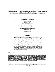
Figure 1: (Left) Automatic layout of the drug effect network without parameters. (Right) Portion of automatic layout with parameters.

Maximum likelihood parameter learning is implemented both for complete data (Nodelman et al., 2003) and for incomplete data (Nodelman et al., 2005) via the expectation-maximization algorithm. Structure learning is also implemented for both complete and incomplete data. The latter represents an implementation of structural expectation maximization. Two structure searches are available: a brute force search that tries all parent sets up to a certain size (not possible for the initial distribution due to acyclic constraints) and a graph edit search that makes local changes to the graph. 3.3 Modularity Any supplied (or user-defined) inference method can be used in expectation-maximization and structural expectation maximization. Different proposal distributions for importance sampling can be added through simple subclassing. Similarly, the code allows for the construction of CTBNs from any underlying process type. As an example, we define “toggle” variables (only the change of state has meaning) through a very short subclass that implements the necessary parameter tieing. This new process can be mixed freely with other processes to create CTBNs of mixed node types. 3.4 Visualization Two visualization tools are supplied. The first converts a CTBN into a text file suitable to be read by the open source package graphviz which can then layout the CTBN in a variety of formats. Figure 1 shows the output of this automatic visualization on the drug effect network from Nodelman et al. (2002). Additionally, either an postscript or text visualization of a trajectory can be automatically generated. Figure 2 shows these outputs for a partially observed trajectory drawn from the same drug effect network.

Acknowledgments This project was supported by the Air Force Office of Scientific Research (FA9550-07-1-0076) and by the Defense Advanced Research Project Agency (HR0011-09-1-0030). We thank Uri Nodelman 1139

S HELTON , FAN , L AM , L EE AND X U

=0

=1

=2

Eating Full Stomach Hungry Uptake Concentration Barometer Joint Pain Drowsy 0.661 1 0.048 0.795 0.053 0.116 0.139 0.375

1.5 1.558 1.611 1.682 1.698

2.396 2.81 2.824 2.993

time \ var 0.000000 0.048261 0.053800 0.116566 0.139465 0.375521 0.661087 0.795507 1.000000 1.500000 1.558340 1.611520 1.682240 1.698080 2.396950 2.810210 2.824950 2.993380

0 0

1 0

2 0 1

3 1

4 0

5 1

6 1

7 0

-1 2

-1 0

-1 0

1 0 1 0 1 -1 1

1 -1 1 2

-1 1

-1 0

-1 1

0 0 0 1 2 1 1

Figure 2: Automatic visualizations of a trajectory of the drug effect network (with all variables missing observations from t = 1 to 1.5), as a postscript file (left) and in text (right).

for sharing his initial implementation of CTBNs and Tal El-Hay for sharing his implementation of Gibbs sampling for CTBNs. Any faults in our software package are purely our own.

References Gunter Bolch, Stefan Greiner, Hermann de Meer, and Kishor S. Trivedi. Queueing Networks and Markov Chains. John Wiley & Sons, Inc., 1998. Gianfranco Ciardo and Andrew S. Miner. A data structure for the efficient Kronecker solution of GSPNs. In Proceedings of the 8th International Workshop on Petri Nets and Performance Models, pages 22–31, 1999. Tal El-Hay, Nir Friedman, and Raz Kupferman. Gibbs sampling in factorized continuous-time Markov processes. In Proceedings of the Twenty-Fourth Conference on Uncertainty in Artificial Intelligence, pages 169–178, 2008. Yu Fan and Christian R. Shelton. Sampling for approximate inference in continuous time Bayesian networks. In Proceedings of the Tenth International Symposium on Artificial Intelligence and Mathematics, 2008. Uri Nodelman, Christian R. Shelton, and Daphne Koller. Continuous time Bayesian networks. In Proceedings of the Eighteenth International Conference on Uncertainty in Artificial Intelligence, pages 378–387, 2002. Uri Nodelman, Christian R. Shelton, and Daphne Koller. Learning continuous time Bayesian networks. In Proceedings of the Nineteenth International Conference on Uncertainty in Artificial Intelligence, pages 451–458, 2003. Uri Nodelman, Christian R. Shelton, and Daphne Koller. Expectation maximization and complex duration distributions for continuous time Bayesian networks. In Proceedings of the Twenty-First International Conference on Uncertainty in Artificial Intelligence, pages 421–430, 2005. Carl A. Petri. Kommunikation mit Automaten. PhD thesis, University of Bonn, 1962. 1140