Continuous-time MAXQ Algorithm for Web Service ... - Semantic Scholar

JOURNAL OF SOFTWARE, VOL. 7, NO. 5, MAY 2012

943

Continuous-time MAXQ Algorithm for Web Service Composition Hao Tang School of Electrical Engineering and Automation, Hefei University of Technology, Tunxi Road No.193, Hefei, Anhui 230009, P.R. China Email: [email protected]

Wenjing Liu, Wenjuan Cheng and Lei Zhou School of Computer and Information, Hefei University of Technology, Tunxi Road No.193, Hefei, Anhui 230009, P.R. China Email: {winnykris, zhouleizhl, wj_cheng}@163.com

Abstract—Web services composition present a technology to compose complex service applications from individual (atomic) services, that is, through web services composition, distributed applications and enterprise business processes can be integrated by individual service components developed independently. In this paper, we concentrate on the optimization problems of dynamic web service composition, and our goal is to find an optimal composite policy. Different from many traditional composite methods that do not scale to large continuous-time processes, we introduce a hierarchical reinforcement learning technique, i.e., a continuous-time unified MAXQ algorithm, to solve large-scale web service composition problems in the context of continuous-time semi-Markov decision process (SMDP) model under either average- or discounted-cost criteria. The proposed algorithm can avoid the “curse of modeling” and the “curse of dimensionality” existing in the optimization process. Finally, we use a travel reservation as an example to illustrate the high effectiveness of the proposed algorithm, and the simulation results show that, it has better optimization performance and faster learning speed than the flat Q-learning. Index Terms—web service composition, hierarchical reinforcement learning, semi-Markov decision process (SMDP), MAXQ

I. INTRODUCTION Web services are considered as self-contained, selfdescribing, and plat-form-independent applications that can be published (Web Services Description Language, WSDL), discovered (Universal Description Discovery and Integration, UDDI) and invoked (Simple Object Access Protocol, SOAP) over the internet [1, 2]. A single web service usually can not fulfill the requirements of a user, while web service compositions provide a way to combine a set of simple web services into more powerful services or new value-added services that can satisfy the user’s needs. So, in modern high-tech world, web service Partially supported by the Nature Science Foundation of Anhui Province (090412046), the Nature Science Foundation of Education Department of Anhui Province (KJ2008A058), and the Humanities and Social Sciences Project of Ministry of Education (09YJA630029)

© 2012 ACADEMY PUBLISHER doi:10.4304/jsw.7.5.943-950

composition has played more and more important role in many domains, typically in e-commerce and enterprise application integration, and has attracted many researchers’ attention. The composition process of web services has been divided into static and dynamic [3, 4]. Static composition is purely manual, whose process model should be built before run time, and each web service is executed one by one so as to achieve the desired requirement. It is a timeconsuming task that requires a lot of effort. However, web service requests are always stochastic, and the environment in which web service composition operation is often dynamic. So, it is inappropriate to select and compose web services statically in such cases, and the dynamic composition process is more competitive. The later creates a process model and selects primitive (atomic) services automatically during the run time, so as to make the composite service adaptable in a high dynamic environment. In this paper, we consider the dynamic web service composition and focus on how to compose services according to a user’s request as well as some quality of service (QoS) properties, that is, given a set of possibly candidate web services and an optimization goal, how to achieve this goal by composing these web services into a web process (workflow) [2]. The QoS model for web service usually includes reliability, cost, response time, availability, and so on. So far, a number of methods have been proposed to achieve dynamic web service composition. For example, Gao et al. has discussed a composition method based on Markov decision process (MDP) [5], and introduced two value iteration algorithms for computing the optimal policy: one is backward recursive iteration and the other is forward iteration. But both algorithms are numerical and model-based, which suffers from the curse of modeling, and can not be used in a model-free case. In [6], a new algorithm is applied for dynamic service composition based on reinforcement learning (RL) and logic of preference. However, in large-scale web service composition problems, current tabular reinforcement learning methods suffer from the “curse of

944

JOURNAL OF SOFTWARE, VOL. 7, NO. 5, MAY 2012

dimensionality” [7], which is the exponential growth of computational and memory requirements with the number of system state variables. So, the method proposed in [6] may encounter low efficiency in the case of a large number of candidate services, although it can realize composition automatically in a model-free case. Typically, any element of a web process may be either a primitive web service or a composition of primitive web services, which itself is a web process. To that end, the web service composition problem as a task can be recursively decomposed into smaller and smaller subtask until reach the primitive tasks. In other words, realistic web processes may be nested as higher level web processes and lower level web processes, in which a higher level web process maybe composed from lower level web processes [8]. Thus, the large-scale web service composition problems can be solved by hierarchical methods [9–11]. One of the ways is to utilize hierarchical reinforcement learning. Wang et al. has adapted MAXQ algorithm to dynamic service composition, which is based on discrete-time semi-Markov decision process (DT-SMDP) [11]. But in real-word applications, web service compositions are always related to run time. Specifically, the performance of a composition process is affected by the real time of network transmission and service processing, which is related to one of the QoS properties, i.e., the response time. Therefore, it is more practical to use continuoustime hierarchical reinforcement learning (HRL) algorithms to solve web service composition problems. In this article, we will propose a dynamic web service composition method based on MAXQ algorithm, in the context of continuous-time semi-Markov decision process (CT-SMDP). It is effective in dealing with the “curse of dimensionality” and the “curse of modeling” for practical large-scale service composition. The rest of this paper is organized as follows: Section 2 presents the framework for dynamic web service composition. Section 3 describes the continuous-time MAXQ algorithm for web service composition. Section 4 demonstrates the experimental results of the approach introduced in section 3. And finally, the last section concludes this paper and discusses the possible future work. II. WEB SERVICE COMPOSITION MODEL The framework of the dynamic web composition model is shown in Figure 1 [1].

Figure 1

Web Service Composition Model.

© 2012 ACADEMY PUBLISHER

service

The service composition system has two kinds of participants, service provider and service requester. The former proposes web services for use, and the latter consumes information or services offered by the former. The system also contains the following components: task acceptor, composed service engine, execution engine, service matchmaking, etc. Firstly, the service providers advertise their atomic services at a global market place. Once a service requester submits his requests and the task acceptor accepts the information, the composed service engine will try to solve the requirement by composing the atomic services advertised by the service providers. Then the execution engine will accept the corresponding flow chart, and send the service specification to the service matchmaking, which will find the most appropriate atomic web services and return the information to the execution engine. Finally, the execution engine invokes and executes each atomic service, and the result will be then sent back to the service requester. The dynamic web service composition problem can be modeled as a SMDP [12–15], which is a more general model than MDP. When a composition process evolves to a task node, the composed service engine should decide to select a concrete web service, and the moment of making decision is called decision epoch. Here, we use tn to denote the nth decision epoch with t0 = 0 . If there are l task nodes to be bound in a web service composition problem, the system state s is then defined as a conjunction of status of each task node, i.e., s =< s1 ,..., sk ,..., sl > , where sk corresponds to the kth task node of this service composition. sk = 1 represents that this node is active and has been bound to a concrete web service, while sk = 0 means that this node is not active. Let Φ be the system state space, i.e., s ∈ Φ . At time tn and state sn , the action an is selected from the set of all possible candidate web services A( sn ) , i.e., an ∈ A( sn ) , and write A = ∪ A( sn ) . Then, a stationary policy π represents a mapping from states to actions, i.e., π : Φ → A . Here we use the reliability of a relative service as the transition probability p ( sn +1 | sn , an ) [9], that is, under a concrete action an , the system transits from current state sn to next state sn +1 with probability p ( sn +1 | sn , an ) or still stays at state sn with probability 1 − p( sn +1 | sn , an ) . Let τ ss ' be the interval time between tn and tn +1 , and it can also be called the sojourn-time of state sn under action an , which follows a random distribution. Then, the web service composition problem can be modeled as a SMDP. Suppose that the expected cost the system pays every unit time at state sn under action an and before transiting to next state sn +1 is denoted by f ( sn , an , sn +1 ) . Then, we take the following infinite-horizon expected cost criteria [15].

JOURNAL OF SOFTWARE, VOL. 7, NO. 5, MAY 2012

945

ηαπ (s) = E ⎡ ∑ ∫tt α e−αt f (sn , an , sn+1 )dt | s0 = s⎤ , ∀s ∈Φ . (1) ∞

⎢⎣n=0

n +1

n

⎥⎦

Here, α denotes a discount factor, and when α > 0 , η ( s ) represents the long-run expected total discounted cost of states under policy π . As a special case, if α → 0 , the limitation η0π ( s ) represents the following infinite-horizon expected average cost π α

……

V π (i, s )

……

(2)

……

1 ⎡N −1 tn+1 E ∑ ∫tn f (sn , an , sn+1 )dt ⎤ . ⎢⎣ n=0 N →∞ t ⎦⎥ N

ηπ = lim

C π (i, s, j )

The MAXQ algorithm is a well-known approach in hierarchical reinforcement learning, which provides a hierarchical decomposition of the given reinforcement learning problem into a set of sub-problems. Ghavamzadeh and Mahadevan has proposed a continuous-time MAXQ algorithm in the context of SMDP [17], which is an extension of the MAXQ method for discrete-time hierarchical reinforcement learning [18,19]. In that work, continuous-time discounted reward MAXQ algorithm and continuous-time average reward MAXQ algorithm were introduced respectively. Based on those work and by using the concept of performance potential, we will propose a unified optimization framework for both cost criteria in this section. To construct MAXQ decomposition for the web service composition problem, we should first identify a set of individual subtasks that we believe important for solving the overall task. More formally, the MAXQ method decomposes the target task M into a set of subtasks {M 0 , M 1 ,..., M m −1} and decomposes a hierarchical policy π into a set of policy {π 0 , π 1 ,..., π m −1 } with π i corresponding to subtask M i . Each subtask M i is a triple < Ti , Ai , Ri > . The termination predicate partitions the state space Φ into a set of active states Si and a set of terminal states Ti . The policy for subtask M i can only be executed if the current state s ∈ Si . Ai is a set of actions that can be performed to achieve subtask M i , with elements being either primitive actions or other subtasks. Ri is the pseudo cost function, which specifies a pseudocost for each transition to a terminal state. In this case, let us define four tasks as follow: z Root. This is the whole web service composition task. z Input. In this subtask, the goal is to get the request information so as to invoke a concrete service. z Output. In this subtask, the goal is to obtain the service output data. z Comp. In this subtask, the goal is to select an appropriate composite model during the composition process. In other words, it is to move the service process from its current state to target state.

© 2012 ACADEMY PUBLISHER

V π ( j, s) ……

III. CONTINUOUS-TIME MAXQ ALGORITHM FOR SERVICE COMPOSITION

Figure 2

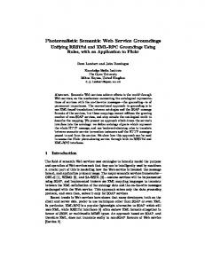
MAXQ graph for the web service composition problem.

By decomposing we can obtain a MAXQ graph for web service composition problem as shown in Figure 2 according to [19]. There are two kinds of nodes: MAX nodes (triangles) and Q nodes (rectangles). A MAX node with no children denotes a primitive action and the one with children represents a composite subtask. The immediate children of each MAX node are Q nodes corresponding to the actions that are available for each subtask. Specifically, each MAX node M i can be viewed as computing the value of V π (i, s ) for its subtask, which is the expected cumulative cost of executing π i and the policies of all descendants of M i starting at state s until M i terminates. For a primitive MAX node, this information is stored in the node, while for a composite MAX node, this information is obtained by the Q node selected by π i . Suppose that the policy π i of M i chooses subtask π i ( s ) = j at state s. Then, each Q node with parent task M i , state s, and child task M j can be viewed as computing the value of Qπ (i, s, π i ( s )) that is equal to the projected value function V π ( j , s ) of its child task M j plus its completion function C π (i, s, j ) . Here, C π (i, s, j ) is stored in the Q node, and represents the expected discounted cumulative cost of completing subtask M i after invoking the subroutine for subtask M j at state s. V π (i , s )

C π (i, s, j )

V π ( j, s)

Execution of Subtask i

sI

s

s'

sT

Execution of Action j

Figure 3

Note how the caption is centered in the column.

The decomposition for the V π (i, s ) is also shown by Figure 3. Each circle is a state of the composition process, and suppose subtask M i is initiated at state sI and terminated at state sT . If i is a primitive action, then s = sI , s ' = sT . The interval time τ ss ' between state s and

946

JOURNAL OF SOFTWARE, VOL. 7, NO. 5, MAY 2012

its next state s ' is the sojourn-time of state s, which is assumed to be exponential distribution during our experiments in the next section. If i is a composite action, τ ss ' is the cumulative time that can be separated into several interval times, and is no longer exponential distribution. Then, the value function V π (i, s ) of state s for M i in the MAXQ algorithm is broken into two parts: the value of the subtask M j that is independent of the parent task M i , and the value for completing M i after executing subtask M j that of course depends on the parent task M i . So, we have

⎧ f '(s, i, s ') V π (i, s) = ⎨ π ⎩Q (i, s, π i (s))

if i is primitive if i is composite

.

(3)

τ

Here, Tα (τ ) = ∫0 e −α t dt =

α

for any discount factor

α > 0 and time τ > 0 , and let T0 (τ ) = αlim Tα (τ ) = τ . In →0 addition, γ is a stepsize, and T is the current total cumulative time for executing subtask M i . Due to the introduction of the term Tα (i) × η in equation (4) and (10) according to the idea of performance potential for SMDP [15, 16], the unified MAXQ algorithm can then be established for both discounted and average criteria, which is the difference between our algorithm and other MAXQ algorithms such as proposed in [14]. The continuous-time unified MAXQ algorithm for web service composition is depicted in Table I, and the flowchart of this algorithm is shown in Figure 4.

where

TABLE I. MAXQ ALGORITHM FOR WEB SERVICE COMPOSITION τ ss '

f '(s, i, s ') = k1 (s, i) + ∫ k2 (s, i, s ') × e−αt dt − Tα (τ ss ' ) ×η .

(4)

0

Qπ (i, s, j) = V π ( j, s) + Cπ (i, s, j) .

(5)

Here, k1 ( s, i ) represents the immediate cost of executing primitive action i at state s, which represents the user’s request in web service composition problem, like the price acceptable, the distance between the hotel and the airport, and so on; k2 ( s, i, s ') represents the time-related cost that the system pays every unit time, such as response time. In addition, η represents the estimate of average cost, satisfying Sf

η :=

Sw

(6)

S f := S f + βn ( fα =0 (s, i, s ') − S f ) .

(7)

Sw := Sw + βn (τ ss ' − Sw ) .

(8)

'

Here, β n is a stepsize, and fα' = 0 ( s, i, s ') is calculated by (4) with α = 0 , which denotes accumulated cost from s to s ' under primitive action i. The projected value function for the root is then decomposed into the ones for the individual subtasks and the individual completion functions recursively by equations (3) to (5). Furthermore, V π (i, s ) and C π (i, s, j ) are updated, respectively, as follows V π (i, s) := (1 − γ )V π (i, s) + γ × f '(s, i, s ') . π

−αT

π

(9)

π

C (i, s, j):= (1−γ )C (i, s, j) +γ (e (C (i, s ', j ') +V ( j ', s ')) −Tα (T) ×η) . (10

) j ' = arg mina '∈A ( s ') (V π (a ', s ') + Cπ (i, s ', a ')) . i

© 2012 ACADEMY PUBLISHER

1. 2.

function CTU_MAXQ(MaxNode i, State s) initialize Stack = {s, i,τ ss ' , f ', fα' = 0 }

3. 4.

if i is primitive MAXNode, then execute action i in state s, receive sojourn-time τ ss ' , observe state s ' ; calculate the accumulated cost f '( s, i, s ') and f 'α = 0 ( s, i, s ') according to (4)

5.

push the sample records into the top of the Stack{} ; calculate

η according to (6)-(8) and compute 6. 7. 8.

the value of V π (i, s )

according to (3)-(5) else while s ∉ Ti do choose action j according to the current ε − greedy policy

πi

.

with s f and sw being learned, respectively, as follows

π

1 − e −ατ

(11)

9. 10.

let ChildStack = CTU_MAXQ(j, s) while executing action j observe result state s '

11.

let j ' = arg min a '∈ Ai ( s ') (C π (i, s ', a ') + V π (a ', s '))

12. 13. 14.

T=0 for the element of the ChildStack from the beginning do T := T + τ ss ' , calculate η and compute C π (i, s ', j ') via (10)

15. end for 16. append ChildStack onto the top of Stack let s = s ' 17. 18. end while 19. end if 20. return Stack 21. end CTU_MAXQ 22. initialize V π (i, s ) and C π (i, s, j ) arbitrarily 23. CTU_MAXQ (0, s0 )

IV. EXPERIMENTS In web service composition problems, a complete web service composition task is staring from service requester submitting requests to the system returning the results. After finishing a web service composition task, it will deal with another web service composition task immediately. In this section, we will demonstrate the high

JOURNAL OF SOFTWARE, VOL. 7, NO. 5, MAY 2012

947

viewpoint, which constitute the second level. Then they all decompose into three subtasks: find, select, book respectively. At last level, there are all primitive actions which are the candidate web services that can be bound to the corresponding parent task node. The goal is to find an optimal composite policy according to user’s request.

Figure 4

Flow chart for the continues-time MAXQ algorithm.

effectiveness of the continues-time unified MAXQ method by using a travel reservation as a simulation example.

A. Simulation model Let us assume that a customer wants to travel to someplace. So he/she should first tell the travel agent who notes the customer’s requests and generates a corresponding trip request document that may contain several needed plane/train/bus tickets, hotels, car rental, excursions, etc. The travel agent performs all bookings and when he is done, he puts the trip request either into the canceled requests or the completed requests data base. A completed document is sent to the customer as an answer to his request. If the booking fails, the customer is contacted again and the whole process re-iterates. Service providers (airlines, bus companies, hotel chains, etc) are providing web services for selection, and credit card companies are also providing services to guarantee payments made by consumers.

0.65 Q-learning MAXQ

0.6 0.55 0.5 Average cost

η η

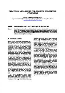
B. Experimental Results As a case study, we suppose there are three web service classes, such as hotel, traffic and viewpoint, and the number of candidate services for each web service class is 10, as shown in figure 5. For comparison, we firstly used flat Q-learning to simulate this problem. In Qlearning, ε − greedy actions are necessary for exploration, especially at the beginning of the optimization. So we use ε = 0.3 , learning step γ = 1 / (8 × N ( s, i )0.2 ) . Here N ( s, i ) is the number of stateaction pairs ( s, i ) that has been visited. k1 ( s, i ) is different for every state-action pairs ( s, i ) , and k2 ( s, i, s ') = 0.8 . First, we consider the average case, i.e., α = 0 . Two optimization plots are provided respectively in Figure 6, where each y-axis denotes the average cost of each algorithm in 1000 episodes. In this problem, a simulation episode is staring from any state to the termination state. We observed that, comparing with the Q-learning, the performance of the MAXQ method is more efficient. The reason is that the MAXQ method accelerates the learning speed and also improved the optimizing precision via

0.45 0.4 0.35 0.3 0.25 0.2

0

Figure 6

100

200

300

400 500 600 Number of iterations

700

800

900

1000

Real time Average cost of the Q-learning and MAXQ algorithm.

0.65 Q-learning MAXQ

0.6 0.55

Discounted costs

0.5 0.45 0.4 0.35 0.3

Figure 5

travel reservation model.

0.25 0.2

As Figure 5 shows, the travel reservation problem is decomposed into 4 levels. The highest level is the task of input, composition and output. Further more, the composition task is decomposed into hotel, traffic and © 2012 ACADEMY PUBLISHER

0

Figure 7

100

200

300

400 500 600 Number of iterations

700

800

900

1000

Real time Discounted costs of Q-learning and MAXQ algorithm ( α = 0.01 ).

948

JOURNAL OF SOFTWARE, VOL. 7, NO. 5, MAY 2012

Q-learning MAXQ

0.55 0.5 0.45 0.4 0.35 0.3 0.25 0.2

0

300

400 500 600 Number of iterations

700

800

900

1000

Q-learning MAXQ

0.8 Success rate of service composition

0.4

0.35

0.25

0

100

200

300

400 500 600 Number of iterations

700

800

900

1000

In addition, we also executed Monte-Carlo policy evaluation for each greedy policy yielded by these two algorithms at every 5 steps, respectively. Specifically, in order to evaluate the relevant performance values, we receive greedy policies at intervals of 5 steps, and then simulated the system by running 1000 steps according to each policy, respectively. Figure 8 and Figure 9 show the results which correspond to Figure 6 and Figure 7, respectively. From those two figures, we can see that the evaluated value of Q-learning method is higher than the MAXQ algorithm both in average and discounted case. From many independent and repeated runs, we conclude that such a unified MAXQ algorithm usually outperforms the flat Q-learning method. On the other hand, we extended the number of tasks to test the other performance values, such as the success rate and the computation cost. The success execution rate Succ( si ) of web service si is a measure related to hardware and/or software configuration of web services and the network connections between the service requesters and providers. Succ( si ) is computed from data of past invocations using the follow expression Succ(si ) = Nc (si ) / K .

(12)

where N c ( si ) is the number of times that service si has been successfully completed, and K is the total number of invocations. So, we define the success rate Succ(π ) of a current policy π is calculated as follow

© 2012 ACADEMY PUBLISHER

0.7 0.6 0.5 0.4 0.3 0.2 0.1

Policy evaluation of Q-learning and MAXQ algorithm for average case.

0

10

20

30

40 50 Number of task

60

70

80

Figure 10 The web service composition success rates of both algorithms with different number of tasks. 15 Q-learning MAXQ

Computation cost(in seconds)

Average costs

200

0.9

0.3

Figure 8

100

Policy evaluation of Q-learning and MAXQ algorithm for discounted cases ( α = 0.01 ).

0.45

0.2

Q-learning MAXQ

0.6

Figure 9

0.55

0.5

0.65

Discounted costs

hierarchy and action abstractions. Figure 7 shows the results of Q-learning and MAXQ algorithm for discounted cases with the discount factor α = 0.01 . As we expected, the graph shows that the MAXQ algorithm can yield a good result faster than Qlearning. And due to the utilization of discount factor α, the curve for discounted case is flatter than it for average case. At the beginning, the curve of the MAXQ algorithm shows obvious fluctuation for either average case or discounted case. The reason is that each subtask is very different from each other, each of them has to be learned separately at first, then be reused (shared).

10

5

0

10

20

30

40 50 Number of tasks

60

70

80

Figure 11 The computation cost of both algorithms.

l

Succ(π ) = ∏ Succ(si ) .

(13)

i =1

Figure 10 shows the success rates of obtained policy for Q-learning and MAXQ algorithm with different number of tasks, respectively. We can see that the success rates reduce as the number of tasks increased. And when the number of the tasks is 10, the success rates of these two algorithms are almost the same. But as the number of the tasks increased, the success rates of Q-learning reduce faster than that of MAXQ algorithm. In addition, the computation costs of both algorithms are shown by Figure 11. Obviously, when the number of tasks becomes large, the computation cost of Q-learning grows faster

JOURNAL OF SOFTWARE, VOL. 7, NO. 5, MAY 2012

949

than that of MAXQ algorithm. These two figures fully illustrate that the MAXQ algorithm is more effective in large-scale service composition problems. The differences for the two algorithms are also listed in Table II. The average cost obtained by Q-learning is 0.2746, while the average cost obtained by MAXQ algorithm is 0.2311, which is almost 15.8% less. The reason is that policies learned in subproblems can be reused for multiple parent tasks, so the optimization performance has been improved. As we known, the MAXQ algorithm is more complex than Q-learning, so the time of completing a certain number of steps for MAXQ algorithm is more than for Q-learning. On the other hand, the value functions learned in subproblems can be shared, so when the subproblem is reused in a new task, learning of the overall value function for the new task is accelerated. When the curves tend to smooth, we consider that the algorithm get a good result. So we can see that the time spent for getting good results by MAXQ algorithm is about 26.4% less than that by Q-learning, as shown in Table II. Furthermore, because of state abstraction, the overall TABLE III. COMPARISON OF DIFFERENT ALGORITHMS

Algorithms

Q-learning

MAXQ

Average cost

0.2746

0.2311

Time for 1000 steps

1.6688 s

1.7661 s

Time for getting good results

1.3678 s

1.0067 s

value function can be represented compactly as the sum of separate terms that each depends on only a subset of the state variables. This more compact representation of the value function will require less data to learn, so as to improve the learning speed. For comparing with Qlearning, we define the reduction rate of memory units q for MAXQ algorithm as q = ((C − B) / C ) × 100% . Here B is the number of memory units that MAXQ algorithm required, and C is the number of memory units that Qlearning required. In the model we proposed, the value of q is (1 − (8 + 8 × N + N × W ) (3 × N × W )) × 100% with N being the number of tasks and W being the number of candidate services. According to this formula, we can obtain the limit of q is 66.67% when W tend to infinity and N is fixed, or the limit is (1 − (8 + W ) (3 × W )) × 100% when N tend to infinity and W is fixed. And the relation between q and N, W is shown in Table III. From Table III, we can see that by applying state abstraction, the MAXQ required much less memory units than Q-learning. Obviously, q increases as the number of tasks and candidate services increased. It fully demonstrates that the MAXQ algorithm is more applicable to large-scale web services composition problems.

© 2012 ACADEMY PUBLISHER

TABLE II. REDUCTION RATES OF MEMORY UNITS FOR MAXQ ALGORITHM COMPARING WITH Q-LEARNING (%).

V. CONCLUSIONS The web service composition problems, under either average- or discounted-cost criteria, are solved effectively by using continues-time unified MAXQ algorithm. Compared with Q-learning, the proposed algorithm tends to be more suitable for solving the “curse of dimensionality” in large-scale web service composition problems. The simulation results also demonstrated that the MAXQ algorithm has the advantages of high effectiveness and high learning speed. In our work, our optimization goal is concerned about the price requirements of user. But the algorithm we proposed in this paper can also apply to other elements of QoS issues like reliability. In addition, as part of our ongoing work, we will extend our algorithm to support multi-agent web service composition problems. REFERENCES [1] J. Rao, X. Su, “A Survey of Automated Web Service Composition Methods”, Proceedings of the First International Workshop on Semantic Web Services and Web Process Composition, 2004, pp. 43-54. [2] H. Zhao, and P. Doshi, “Composing Nested Web Processes Using Hierarchical Semi-Markov Decision Process”, AAAI Workshop on AI-Driven Technologies for servicesOriented Computing, pp. 75-84, 2006. [3] F. H. Khan, S. Bashir, M. Y. Javed, A. Khan, M. S. H. Khiyal, “QoS Based Dynamic Web Services Composition & Execution”, Pages IEEE format, International Journal of Computer Science and Information Security, IJCSIS, vol. 7 no. 2, pp. 147-152, USA, February 2010. [4] F. Mustafa, T. L McCluskey., “Dynamic Web Service Composition”, International Conference on Computer Engineering and Technology, 2009. [5] A. Gao, D. Yang, S. Tang, and M. Zhang, “Web Service Composition Using Markov Decision Processes”, International Conference on Web-Age Information Management, 2005, pp. 308-319. [6] H. B. Wang, P. P. Tang, P. Hung, “RLPLA: A reinforcement learning Algorithm of Web service Composition with Preference Consideration”, IEEE Congress on Services Part II, pp. 163-170, 2008. [7] G. B. Andrew, S. Mahadevan, “Recent Advances in Hierarchical Reinforcement Learning”, Discrete Event Dynamic Systems, vol.13 no.1-2, pp.41-77, 2003. [8] H. Zhao, P. Doshi, “A hierarchical framework for composing nested web processes”, International Conference on Service Oriented Computing, 2006. [9] E. Sirin, B. Parsia, D. Wu, J. Hendler, D. Nau, “HTN planning for Web Service composition using SHOP2”,

950

[10]

[11] [12]

[13]

[14] [15] [16]

[17]

[18] [19]

JOURNAL OF SOFTWARE, VOL. 7, NO. 5, MAY 2012

Web Semantics: Science, Services and Agents on the World Wide Web, pp. 377-396, 2004. K. Chen, J. Y. Xu, S. Reiff-Marganiec, “Markov-HTN Planning Approach to Enhance Flexibility of Automatic Web Service Composition”, IEEE International Conference on Web Services, 2009, pp. 9-16. H. B. Wang, X. H. Guo, “Preference-Aware Web Service Composition Using Hierarchical Reinforcement Learning”, Web Intelligence/IAT Workshops, pp. 315-318, 2009. S. J. Bradtke, and M. O. Duff, “Reinforcement learning methods for continuous-time Markov decision problems”, in Advances in Neural Information Processing Systems 7, Cambridge, MA: MIT Press, pp. 393-400, 1995. S. Mahadevan, N. Marchalleck, T. Das, A. Gosavi, “Selfimproving factory simulation using continuous-time average-reward reinforcement learning”, Proceedings of the 14th International Conference on Machine Learning, 1997, pp. 202-210. R. Parr, “Hierarchical control and learning for Markov decision processes”, PhD Thesis, University of California at Berkeley, 1998. X. R. Cao, “Semi-Markov decision problems and performance sensitivity analysis”, IEEE Transactions on Automatic Control, 48(5): 758-769, 2003. H. Tang, T. Arai, “Look-ahead control of conveyorserviced production station by using potential-based online policy iteration”, International Journal of Control, 82(10): 1916-1928, 2009. M. Ghavamzadeh, S. Mahadevan, “Continuous-Time Hierarchical Reinforcement Learning”, Proceedings of the Eighteenth International Conference on Machine Learning, 2001, pp. 186-193. T. G. Dietterich, “Hierarchical reinforcement learning with the MAXQ value function decomposition”, Journal of Artificial Intelligence Research, 13:227-303, 2000. T. G. Dietterich, “The MAXQ Method for Hierarchical Reinforcement Learning”, Proceedings of the Fifteenth International Conference on Machine Learning, 1998, pp. 118-126.

© 2012 ACADEMY PUBLISHER

Hao Tang was born in 1972. He received his B.E. degree from Anhui Institute of Technology, P.R. China, in 1995, M.E. degree from Institute of Plasma Physics, Chinese Academy of Sciences, in 1998, and Ph.D. degree from University of Science and Technology of China (USTC) in 2002. He has been a postdoctoral researcher at Advanced Robotics with Artificial Intelligence Lab in The University of Tokyo, Japan, from 2005 to 2007. He is currently a professor of Hefei University of Technology, P.R. China. His research interests include DEDSs, reinforcement learning, the methodology of neuro-dynamic programming, and intelligent optimization.

Wenjing Liu was born in 1985. She received her B.E. degree from Anhui Agricultural University, P.R. China, in 2007, M.E. degree from Hefei University of Technology, P.R. China, in 2011. Her research interests include DEDSs, reinforcement learning.

Lei Zhou was born in 1981. He is currently a lecturer and Ph.D. candidate of Hefei University of Technology, P.R. China. His research interests include DEDSs, reinforcement learning.