This thesis is dedicated to my wife Kathryn Lynn Adcock (née Gillespie) for her pa- .... 3.4.2 Derivation of optimum measurement window . ..... As a point of reference, today's personal or server computers have a word size of 32 or. 64 bits. ..... that unlimited precision real numbers in the physical universe are prohibited by the.
UNIVERSITY OF CALGARY
Continuous-Variable Quantum Computation of Oracle Decision Problems
by
MARK R. A. ADCOCK
A THESIS SUBMITTED TO THE FACULTY OF GRADUATE STUDIES IN PARTIAL FULFILLMENT OF THE REQUIREMENTS FOR THE DEGREE OF DOCTOR OF PHILOSOPHY
DEPARTMENT OF PHYSICS AND ASTRONOMY INSTITUTE FOR QUANTUM INFORMATION SCIENCE
CALGARY, ALBERTA DECEMBER, 2012
c MARK R. A. ADCOCK 2012 �
Abstract Quantum information processing is appealing due its ability to solve certain problems quantitatively faster than classical information processing. Most quantum algorithms have been studied in discretely parameterized systems, but many quantum systems are continuously parameterized. The field of quantum optics in particular has sophisticated techniques for manipulating continuously parameterized quantum states of light, but the lack of a code-state formalism has hindered the study of quantum algorithms in these systems. To address this situation, a code-state formalism for the solution of oracle decision problems in continuously-parameterized quantum systems is developed. In discrete-variable quantum computation, oracle decision problems exploit quantum parallelism through the use of the Hadamard transform. The challenge in continuousvariable quantum computation is to exploit similar quantum parallelism by generalizing the Hadamard transform to the continuous Fourier transform while avoiding nonrenormalizable states. This straightforward relationship between the operators in the discrete and continuous settings make oracle decision problems the ideal test-bed. However, as the formalism results in a representation of discrete information strings as proper code states, the approach also allows for the study of a wider range of quantum algorithms in continuously-parameterized quantum systems having both finite- and infinitedimensional Hilbert spaces. In the infinite-dimensional case, we study continuous-variable quantum algorithms for the solution of the Deutsch–Jozsa oracle decision problem implemented within a single harmonic-oscillator. Orthogonal states are used as the computational bases, and we show that, contrary to a previous claim in the literature, this implementation of quantum information processing has limitations due to a position-momentum trade-off of the Fourier transform. We further demonstrate that orthogonal encoding bases are ii
iii not unique, and using the coherent states of the harmonic oscillator as the computational bases, our formalism enables quantifying the relative performances of different choices of the encoding bases. We extend our formalism to include quantum algorithms in the continuously parameterized yet finite-dimensional Hilbert space of a coherent spin system. We show that the highest-squeezed spin state possible can be approximated by a superposition of two states thus transcending the usual model of using a single basis state as algorithm input. As a particular example, we show that the close Hadamard oracle-decision problem, which is related to the Hadamard codewords of digital communications theory, can be solved quantitatively more efficiently using this computational model than by any known classical algorithm.
Acknowledgements This thesis is dedicated to my wife Kathryn Lynn Adcock (n´ee Gillespie) for her patience and perseverance through the many hours I have spent on this research and thesis preparation. Without her continual support, this thesis would not have been written. I would also like to give special thanks to my father Antony Herbert Martin Adcock and my mother Heather Dawn Adcock (n´ee Penrose) for giving me the motivation to undertake this endeavour. It is not clear where the motivation to do a part-time Ph.D. comes from. I think it emerges or is incubated from a young age where one is taught to wonder at the things around us. From watching a chrysalis, to thinking how a radio works, to the joys of algebra, the motivation was instilled in me at a young age. I would also like to express my gratitude to my supervisors Dr. Barry Sanders and Dr. Peter Høyer. We have enjoyed many discussions over the last 7 years, and they have taught me the importance of perspective in the multi-disciplinary field of quantum information. Both supervisors have also instilled in me an appreciation of the English language and, perhaps more importantly, writing for the reader and not just for myself. I hope that this thesis reflects that as well. I would also like to thank our children Katie, Keith and Stephen for their understanding and patience over the years. Finally, I would like to express my gratitude to General Dynamics Canada for their support.
iv
v
Table of Contents Abstract . . . . . . . . . . . . . . . . . . . . . . . . . . . . . . . . . . . . Acknowledgements . . . . . . . . . . . . . . . . . . . . . . . . . . . . . . Table of Contents . . . . . . . . . . . . . . . . . . . . . . . . . . . . . . . List of Symbols . . . . . . . . . . . . . . . . . . . . . . . . . . . . . . . . List of Figures . . . . . . . . . . . . . . . . . . . . . . . . . . . . . . . . . 1 INTRODUCTION . . . . . . . . . . . . . . . . . . . . . . . . . . . 1.1 Introduction . . . . . . . . . . . . . . . . . . . . . . . . . . . . . . . 1.2 Discrete computation . . . . . . . . . . . . . . . . . . . . . . . . . . 1.2.1 Discrete classical computation . . . . . . . . . . . . . . . . . 1.2.2 Discrete quantum computation . . . . . . . . . . . . . . . . 1.3 Continuous computation . . . . . . . . . . . . . . . . . . . . . . . . 1.3.1 Continuous classical computation . . . . . . . . . . . . . . . 1.3.2 Continuous quantum computation . . . . . . . . . . . . . . . 1.4 Thesis organization . . . . . . . . . . . . . . . . . . . . . . . . . . . 2 BACKGROUND . . . . . . . . . . . . . . . . . . . . . . . . . . . . 2.1 Introduction . . . . . . . . . . . . . . . . . . . . . . . . . . . . . . . 2.2 The quantum advantage . . . . . . . . . . . . . . . . . . . . . . . . 2.2.1 The advantage with discrete variables . . . . . . . . . . . . . 2.2.2 The advantage with continuous variables . . . . . . . . . . . 2.3 Coherent states . . . . . . . . . . . . . . . . . . . . . . . . . . . . . 2.3.1 Coherent states of the harmonic oscillator . . . . . . . . . . 2.3.2 Coherent spin states . . . . . . . . . . . . . . . . . . . . . . 2.3.3 Continuous representations . . . . . . . . . . . . . . . . . . . 2.4 Spectrum of measurement . . . . . . . . . . . . . . . . . . . . . . . 2.5 Oracle-decision Problems . . . . . . . . . . . . . . . . . . . . . . . . 2.5.1 Definition . . . . . . . . . . . . . . . . . . . . . . . . . . . . 2.5.2 The Deutsch–Jozsa oracle decision problem . . . . . . . . . . 2.6 Algorithms for solving the Deutsch–Jozsa problem . . . . . . . . . . 2.6.1 The classical version of the Deutsch–Jozsa algorithm . . . . 2.6.2 The traditional (n + 1) qubit Deutsch–Jozsa algorithm . . . 2.6.3 The two-mode continuous-variable Deutsch–Jozsa algorithm 2.7 Summary . . . . . . . . . . . . . . . . . . . . . . . . . . . . . . . . 3 QUANTUM COMPUTATION WITH ORTHOGONAL STATES . 3.1 Introduction . . . . . . . . . . . . . . . . . . . . . . . . . . . . . . . 3.2 An n-qubit quantum Deutsch–Jozsa algorithm . . . . . . . . . . . . 3.3 Single mode continuous-variable algorithm with orthogonal states . 3.3.1 Continuous-variable model selection . . . . . . . . . . . . . . 3.3.2 Encoding Information into Orthogonal States . . . . . . . . 3.4 Bounding the success probability . . . . . . . . . . . . . . . . . . . 3.4.1 Proof of dominance of antisymmetric balanced function . . . 3.4.2 Derivation of optimum measurement window . . . . . . . . .
. . . . . . . . . . . . . . . . . . . . . . . . . . . . . . . . . . . . . . . . .
. . . . . . . . . . . . . . . . . . . . . . . . . . . . . . . . . . . . . . . . .
. . . . . . . . . . . . . . . . . . . . . . . . . . . . . . . . . . . . . . . . .
ii iv v vii viii 1 1 6 6 9 13 13 15 18 21 21 22 22 24 28 29 33 36 40 42 42 43 44 44 45 49 51 53 53 54 58 59 66 70 71 74
3.4.3 Numerical value of single-query success probability . . . . . . . . 77 3.4.4 Success probability after multiple repetitions . . . . . . . . . . . . 78 3.5 Summary . . . . . . . . . . . . . . . . . . . . . . . . . . . . . . . . . . . 80 4 QUANTUM COMPUTATION WITH COHERENT STATES . . . . . . 82 4.1 Introduction . . . . . . . . . . . . . . . . . . . . . . . . . . . . . . . . . . 82 4.2 Single mode continuous-variable algorithm with Gaussian states . . . . . 84 4.2.1 Encoding information into Gaussian states . . . . . . . . . . . . . 86 4.3 Bounding the success probability with Gaussian States . . . . . . . . . . 89 4.3.1 Proof of dominance of symmetric and antisymmetric functions . . 90 4.3.2 Numerical value of single-query success probability . . . . . . . . 98 4.4 Summary . . . . . . . . . . . . . . . . . . . . . . . . . . . . . . . . . . . 103 5 QUANTUM COMPUTATION WITHCOHERENT SPIN STATES . . . 107 5.1 Introduction . . . . . . . . . . . . . . . . . . . . . . . . . . . . . . . . . . 107 5.2 The Close Hadamard Oracle Decision Problem . . . . . . . . . . . . . . . 109 5.2.1 Codewords with unrestricted errors . . . . . . . . . . . . . . . . . 111 5.2.2 Codewords with restricted errors . . . . . . . . . . . . . . . . . . 111 5.2.3 Approach to solution using coherent spin states . . . . . . . . . . 113 5.3 Spin System Model . . . . . . . . . . . . . . . . . . . . . . . . . . . . . . 114 5.3.1 Input state preparation . . . . . . . . . . . . . . . . . . . . . . . . 116 5.4 Efficient Algorithm for the Close Hadamard Problem . . . . . . . . . . . 122 5.4.1 Algorithm Response to the Hadamard Codewords . . . . . . . . . 123 5.4.2 Solution of the Close Hadamard Problem . . . . . . . . . . . . . . 130 5.4.3 Classical Algorithm . . . . . . . . . . . . . . . . . . . . . . . . . . 131 5.5 Alternative Algorithm . . . . . . . . . . . . . . . . . . . . . . . . . . . . 132 5.6 Summary . . . . . . . . . . . . . . . . . . . . . . . . . . . . . . . . . . . 135 6 SUMMARY AND CONCLUSIONS . . . . . . . . . . . . . . . . . . . . . 137 6.1 Conclusions . . . . . . . . . . . . . . . . . . . . . . . . . . . . . . . . . . 138 6.1.1 Code-state formalism with orthogonal states . . . . . . . . . . . . 138 6.1.2 Code-state formalism with coherent states of the harmonic oscillator139 6.1.3 Code-state formalism with coherent spin states . . . . . . . . . . 139 6.2 Summary of contributions . . . . . . . . . . . . . . . . . . . . . . . . . . 140 6.2.1 Reconciling the regularization problem . . . . . . . . . . . . . . . 141 6.2.2 Construction of a single mode algorithm . . . . . . . . . . . . . . 142 6.2.3 Techniques for bounding success probability . . . . . . . . . . . . 143 6.2.4 Continuous-variable algorithms in finite-dimensional Hilbert spaces 144 6.3 Future research . . . . . . . . . . . . . . . . . . . . . . . . . . . . . . . . 144 6.3.1 Physical implementation . . . . . . . . . . . . . . . . . . . . . . . 144 6.3.2 Tightening the bound on the single-query success probability . . . 147 6.3.3 Explore operator/codeword symmetries in spin setting . . . . . . 147 6.4 Closing Remarks . . . . . . . . . . . . . . . . . . . . . . . . . . . . . . . 147 Bibliography . . . . . . . . . . . . . . . . . . . . . . . . . . . . . . . . . . . . 149
vi
List of Symbols |α� |θ, φ�s δ δ(x − x� ) f m n N P φ ˜ φ(p)
φ(x)
|p� Pr⊥ � Pr�� |ψ� θ |x�
A coherent state of the harmonic oscillator. 30, 31 A coherent spin state of a spin system having 2s + 1 spin states. 34 Half-width of position measurement window. 64, 73, 141 The Dirac-delta functional also expressed as �x|x� �. 25 A Boolean function that takes an n-bit input and gives a single bit output. 42 An integer that represents the number of times an oracle is queried or an algorithm is called. 43 An integer that represents the number of bits or qubits used as function or algorithm input. 42 There are a total of N = 2n n-bit strings. 42, 63 Region of momentum domain encoded with discrete information. 59, 64 Spherical coordinate for angle of longitude. vii, 34 Momentum representation of the wave function into which information is encoded. The momentum wave function is the Fourier transform of the position wave function φ(x). 30 Position representation of the wave function employed as the input state of continuous-variable algorithms. The position wave function is the inverse Fourier transform of the momentum wave ˜ function φ(p). 30 Continuous-variable momentum state is an eigenstate of the momentum operator pˆ with eigenvalue p ∈ R . |p� is the Fourier transform of |x�. 25 Single query success probability for the continuous-variable algorithm employing orthogonal states. 74, 81, 137 Single query success probability for the continuous-variable algorithm employing Gaussian states. 81, 137 Dirac representation of the position wave function ψ(x) = �x|ψ�. 27 Spherical coordinate for angle of latitude. vii, 34 Continuous-variable position state is an eigenstate of the position operator xˆ with eigenvalue x ∈ R . |x� is the Fourier transform of |p�. 25
vii
List of Figures 1.1 1.2
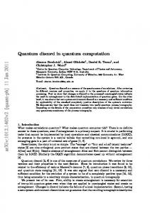
The four forms of computation and their respective variables. . . . . . . . Quantum circuit implementing the two-qubit CNOT gate. . . . . . . . . .
5 11
2.1 2.2 2.3 2.4 2.5
Wigner functions for vacuum and squeezed state . . . . . . . . . . . . . Wigner function for the sinc wave function . . . . . . . . . . . . . . . . Spherical Q-function of a coherent spin state . . . . . . . . . . . . . . . Traditional (n + 1)-qubit circuit for the Deutsch–Jozsa algorithm. . . . Two-mode continuous-variable circuit for the Deutsch–Jozsa algorithm.
. . . . .
37 39 40 45 49
3.1 3.2 3.3 3.4 3.5 3.6 3.7 3.8 3.9
Alternative n-qubit circuit for the Deutsch–Jozsa algorithm. . . . . . . . Single mode continuous-variable circuit for the Deutsch–Jozsa algorithm Illustration of information encoding . . . . . . . . . . . . . . . . . . . . . Overview of the steps in the single-mode continuous-variable algorithm . (4) Encoded functions fz (p) . . . . . . . . . . . . . . . . . . . . . . . . . . The phasors eiϕj x . . . . . . . . . . . . . . . . . . . . . . . . . . . . . . . (4) The probability distributions |φz (x)|2 . . . . . . . . . . . . . . . . . . . Definition of the phasor angles for the N = 4 base case for P = 1 . . . . Optimum measurement window using orthogonal wave functions . . . . .
55 60 64 65 68 69 71 73 75
4.1 4.2 4.3 4.4 4.5 4.6
The Gaussian width must be matched to the information width . . . Phasor representation of the Gaussian modulated position state . . . Plots of the magnitude of the position modulation function . . . . . . Optimum measurement window using coherent wave functions . . . . Comparison between the orthogonal and the Gaussian wave functions Wigner functions of encoded coherent states . . . . . . . . . . . . . .
5.1 5.2 5.3 5.4 5.5 5.6 5.7 5.8
Single-mode circuit for solving oracle decision problems in the spin setting Q-function and spin-state distribution for coherent spin state . . . . . . . Q-function and spin-state distribution for squeezed spin state . . . . . . . Variance and spin-state distribution for optimally squeezed spin state . . Squeezed spin-state probability distributions for s = 7/2 to s = 63/2 . . . Symmetric superpositions are preserved for Hadamard codewords . . . . Unrestricted errors result in reduced probability of central components . Alternate discrete Fourier-based algorithm probability distributions . . .
6.1
Physical implementation of the single-mode, continuous-variable algorithm 145
viii
. . . . . .
. 88 . 92 . 97 . 101 . 103 . 105 114 116 118 120 121 123 128 135
1
Chapter 1 INTRODUCTION 1.1 Introduction Perhaps the most significant aspect of quantum computing is the exponential speed-up observed for certain quantum algorithms over their classical counterparts. For example, it is estimated in [1] that the famous Shor factoring algorithm [2] running on a quantum computer has O(n) computational complexity using O(n3 ) qubits to factor an n-digit number. In comparison, the best known classical algorithm, the number field sieve, has O(e(nk log 2n)
1/3 )
) [1] computational complexity using computing resources superpolynomial
in the number of digits. The superpolynomial speed-up of the quantum factoring algorithm has significant ramifications if scalable quantum computers can be made given that security protocols are based on the apparent difficulty of factoring large numbers on classical computers. Note that we use asymptotic notation [3, 4, 5] throughout this thesis for the purpose of comparing the performance of quantum algorithms to classical algorithms. Shor’s algorithm, and most other quantum algorithms, have been studied in discretelyparameterized quantum systems. Discrete-variable quantum systems, where experimentalists have successfully demonstrated the potential computational power of quantum systems, include trapped ions [6], liquid nuclear magnetic resonance [7] and quantum dots [8]. The processing of quantum information in discrete-variable systems has the advantage of being amenable to the theory of quantum error correction. Continuous-variable quantum information is the less studied of the two types of quantum information, but there has been significant progress made in recent years in under-
2 standing and controlling quantum optics systems [9, 10, 11, 12, 13, 14, 15, 16, 17]. Processing with continuous-variable systems thus has the advantage of being amenable to many physical preparation and measurement procedures that feature continuous tunability. However, there is lack of a formalism governing the use of proper code-states that has hindered the study of quantum algorithms in these systems. The absence of a rigorous orthogonal code-state formalism in the continuous-variable model of quantum computing impedes the development of quantum algorithms accompanied by error bounds and full resource analysis. Furthermore the literature on continuousvariable quantum information deleteriously blurs two distinct challenges: finite- vs. infinite-dimensional Hilbert spaces and discrete vs. continuous parameterizations. In addition due to a lack of a code-state formalism, there are examples in the literature where false conclusions of the performance of continuous-variable algorithms have been drawn. In order to develop our formalism, we first need to define what we mean by continuousvariable quantum information. In our study of continuous-variable quantum information, we consider both finite- and infinite-dimensional Hilbert spaces, which are continuously parameterized. We operationally define continuous-variable quantum information in two ways: continuously parameterized preparation and continuously parameterized measurement. In the case of finite-dimensional Hilbert spaces, we use continuously parameterized preparation, but we use discrete measurement. In the case of infinite-dimensional Hilbert spaces, we use continuously parameterized preparation, and we define continuously parameterized measurements in terms of a dense spectrum in the real numbers. Braunstein and Pati [18] attempted to map the discrete quantum algorithm for the solution of the Deutsch–Jozsa [19] oracle decision problem directly to the infinitedimensional, continuous-variable setting. Their claim of infinite speedup of the continuousvariable algorithm over the classical deterministic approach was based on the use of im-
3 proper, non-renormalizable states and was subsequently proven false [20]. Similarly an attempt to encode a qudit into a single harmonic oscillator [21] has been demonstrated to have serious problems making it non-renormalizable as well [22]. The need for a code-state formalism in the infinite dimension setting is clear. We begin by dealing with the infinite-dimensional case. Oracle decision problems have been studied in the discrete quantum setting since the early days of quantum information theory [23]. We select oracle decision problems as the test-bed for our formalism because in the discrete case, they exploit quantum parallelism through the application of the Hadamard transform. The challenge of continuous-variable quantum computation is exploiting the same parallelism by generalizing the Hadamard transform to the continuous Fourier transform yet avoiding having non-renormalizable states as computational states in both the canonical position domain and its momentum dual. There is a trade-off, and the lessons from studying oracle decision problems will be valuable elsewhere in the study of continuous-variable quantum information processing. We select the Deutsch–Jozsa [19] problem as the specific example of an oracle decision problem. The Deutsch–Jozsa [19] algorithm is an important early quantum algorithm that demonstrates exponential speedup over its classical deterministic counterpart. It has also been studied in the continuous-variable setting [18]. The structure of quantum algorithms solving oracle decision problems is quite simple. Typically the input state is a computational basis state. It is transformed into an equal superposition of basis states; the oracle acts on the superposition, which is then transformed back to the computational basis for measurement. Each of the transformations used in the discrete setting has an analogue in the continuous-variable setting. In the infinite-dimensional, continuous-variable setting, the simplest computational model is to use a single mode of the harmonic oscillator. This requires adaptation of the traditional representation of the quantum algorithms employed
4 in the solution of oracle decision problems. Traditional quantum algorithms for the solution of oracle decision problems use n control qubits and a single target qubit [5]. The most straightforward mapping onto harmonic oscillators thus requires two oscillators. As we wish to use a single oscillator, our novel approach is first to map the traditional quantum algorithm to one employing only n-qubits by removing the requirement for the target qubit. We then extrapolate this new discrete quantum algorithm to a single-mode of a harmonic oscillator [20]. Another challenging aspect of our formalism is the problem of encoding finite information into the momentum basis of the harmonic oscillator. We achieve this by defining proper, orthogonal code-states with unique mapping between elements in the code space and each of the bits contained in the n-bit string loaded into the oracle. We demonstrate that orthogonal encoding bases are not unique, and our formalism enables quantifying the relative performances of different choices of the encoding bases [24]. The single-mode circuit is also applicable to a continuous parameterization of a collection of spin-1/2 atoms. This novel extension of the formalism to a continuously parameterized system having a finite-dimensional Hilbert space, led to the discovery of a new way of efficiently solving a subset of the bounded-distance decoding problem [25]. We refer to this as the restricted close Hadamard problem. This research is significant because it identifies flaws with continuous-variable algorithms in the literature and addresses these flaws. This work also yields important insight into how to perform quantum optics experiments of continuous-variable quantum computation. Except for the implementation of the oracle, all other aspects of the algorithm can be implemented with the existing tools of quantum options. This work also contributes some mathematical techniques that can be adopted for research in other areas. This includes the technique of using the separation between the constant and worst case balanced functions for bounding the single-query success
5
{0, 1}n Classical discrete
{y1 , . . . , yk } with {yi ∈ R} Classical continuous
(|0�, |1�)⊗n Quantum discrete
|y ∈ R�⊗n Quantum continuous
Figure 1.1: The four forms of computation and their respective variables. Here {y1 , . . . , yk } is a set of real numbers with k ≥ 1 in order to represent that more than one instance of the real number line can be used. probability. Since quantum field theories are continuously parameterized, this work could also be employed in the quantum computation associated with these field theories [26]. In order to gain an appreciation of why continuous-variable quantum computation is challenging, we compare it to other forms of computation in the wider classical and quantum settings. In Figure 1.1, we represent the variables used in the four forms of computation, which range from binary digits in the classical discrete case to continuous position states in the quantum continuous case. In the rest of this introduction, we describe the discrete and continuous versions of both classical and quantum computation. For each of the versions of computation, we describe a relevant model of computation. As there are several models of computation applicable to each version, we select the models that most directly relate to our studies of continuous-variable quantum computation. For each version of computation, we discuss the conditions of universal computation for the selected model, the types of problems solved by the model, error correction techniques employed, and extending the elements of computation. In Sec. 1.3, we discuss some of the problems associated with computation based on real numbers. For the case of continuous-variable quantum computation, dealing with this problem leads us to the need for a code-state formalism for continuously-parameterized, infinite dimensional sys-
6 tems. We close the introduction with an overview of the thesis organization in Sec. 1.4.
1.2 Discrete computation Discrete classical computations are carried out on elements of finite sets and discrete quantum computations take place in finite-dimensional Hilbert spaces [27, 28]. In this section, we present a comparison of the two versions of computation highlighting both similarities and differences.
1.2.1 Discrete classical computation Due to the ubiquity of the digital computer, computation with bits has become synonymous with discrete classical computation. Bits are binary digits usually represented by the set {0, 1}. Bits may be implemented by means of a two-state device such as, for example, two distinct voltage or current levels allowed by an electronic circuit. Digital computers usually manipulate bits in groups of a fixed size, conventionally named words. The set of strings that can be represented by an n-bit word is written {0, 1}n , and for example for n = 2, {0, 1}2 = {00, 01, 10, 11}.
(1.1)
As a point of reference, today’s personal or server computers have a word size of 32 or 64 bits. In discrete classical computation theory, many models of computation have been developed. Each model has different capabilities and limitations [29, 3]. Examples of computational models are Boolean circuits [29, 3, 4], the finite-state machine, the randomaccess machine, the pushdown automaton, and the Turing machine [29]. The Turing machine [30] is a standard model of computation. We select the Boolean circuit model
7 A B A ∨ B A ∧ B A ⊕ B ¬A 0 0 0 0 0 1 0 1 1 0 1 1 1 0 1 0 1 0 1 1 1 1 0 0 Table 1.1: The truth table for the two-input logical gates: OR( ∨), AND(∧), and XOR (⊕) and the single-input gate NOT (¬). of computation for discussion here because the Boolean circuit computational model is most appropriate for direct comparison with the circuit model of quantum computation. A Boolean circuit is a collection of gates having inputs and outputs connected by wires. The wires carry the Boolean values 0 and 1. A logic gate is a device implementing a Boolean function. Logic gates come in two forms: two-wire gates and single-wire gates. The basic two-wire gates are the AND, OR and XOR (exclusive OR) gates, and the single wire gate is the NOT gate. For the inputs A, B ∈ {0, 1}, the logical truth tables for these gates are presented in Table 1.1 [4]. Two other important two-wire gates are the NAND gate, which is an AND gate with negated output, and the NOR gate, which is an OR gate with negated output. A gate, or a set of gates, is considered universal if any Boolean operation can be expressed as a finite sequence of the universal gate or elements from the set [29]. For example, the NAND gate and the NOR gate are both universal gates [29]. The NAND gate is the most ubiquitous in the construction of computers because they are simplest to construct using transistor-to-transistor logic [29]. We note that the sets {AND, NOT} and {OR, NOT} are also universal [29, 3, 4]. These sets are mentioned here because they are analogous to similar sets in the circuit model of quantum computation. Boolean circuits are an important part of the modern digital computer since the “silicon chip”, on which computers are in part based, is a very-large-scale integration of Boolean circuits [3]. The modern digital computer is capable of solving a wide variety
8 of problems, indeed algorithms like the number field sieve [1] for solving the factoring problem execute on modern digital computers. However, the whole notion of how difficult a problem is and what is computable and what is not computable by a digital computer pertains to the study of complexity and computability. These subjects are out of the scope of this thesis. There are many good texts on complexity and the theory of computing for example [3, 4]. When a discrete classical computer exchanges information with another computer or when it reads in information from a physical storage device, there is a chance that data words will be corrupted. Computers deal with this problem through the process of error correction. Classical error-correction techniques include forward error correction using error-resistent codewords [31]. The problem of discriminating between codewords received after transmission over a noisy channel is well known in classical digital coding theory employing linear block codes. Linear block codes include simple repetition codes through the more sophisticated Hadamard and Reed–Solomon codes [32]. Quantum error correcting codes are based upon similar principles to the repetition codes [5]. In discrete classical computation, bits can be generalized to d-dimensional digits called dits. Dits may be implemented by d-state physical devices. We briefly introduce dits here for comparison to their quantum counterparts, which are called qudits. The set of strings comprised of n dits may be represented by the set {0, 1, 2, . . . , d − 1}n . Just as the notation {0, 1}n refers to the set of all n-bit strings consisting of zeros and ones, the notation {0, 1, 2, . . . , d − 1}n refers to the set of all n-dit strings consisting of zeros, ones, twos, up to and including the number d − 1. For example when d = 3 we have, {0, 1, 2}2 = {00, 01, 02, 10, 11, 12, 20, 21, 22},
(1.2)
which has cardinality 32 = 9. A practical example of dits is the case where d = 3, which are referred to as trits or
9 ternary digits [33]. For example, a computer architecture based on a fibre-optic ternary computer using the set {−1, 0, 1}n with dark as 0 and the two orthogonal polarizations of light as 1 and -1 has been proposed [33]. In the next subsection, we discus discrete computation with the quantum analogue of the classical bit. Commonly referred to as the qubit [5], the quantum bit is the basic unit of quantum information.
1.2.2 Discrete quantum computation The qubit represents the simplest quantum mechanical system. A qubit has a twodimensional state space. The state space is equipped with an inner product and is referred to as an inner product space. In the finite-dimensional complex vector space employed in discrete quantum computation, a Hilbert space is exactly the same thing as an inner product space [5]. The two computational basis states of the qubit are conventionally written as the vectors (or kets) |0� and |1�. In a classical system, a bit would have to be in one state or the other, but quantum mechanics allows the qubit to be in a superposition of both basis states simultaneously [5]. The superposition is expressed as |ψ� = α|0� + β|1�,
(1.3)
subject to the constraint |α|2 + |β|2 = 1. The ability to create superpositions is fundamental to quantum computing and is the source of much of the advantage of algorithms implemented in quantum systems. This advantage is sometimes referred to as quantum parallelism, which is the ability of quantum computers to perform computations simultaneously [23]. In vector spaces of higher dimension, the states are expressed in a manner analogous to classical systems. For example, a two-qubit system has the computational basis states
10 expressed as |00�, |01�, |10�, |11�, which is analogous to the representation of the values of two-bits given in Eq. (1.1). These basis vectors are frequently expressed using the Kronecker product notation; thus |00� = |0� ⊗ |0� = |0�⊗2 . This notation is extended to define an n-qubit state as |0�|0� · · · |0� = |00 · · · 0� = |0�⊗n .
(1.4)
Any two-level quantum system can be used as a qubit. Multilevel systems can be used as well if two distinct states can be decoupled from the rest [5]. Quantum computation also has models of computation including the circuit model and the one-way quantum computation model [34]. The circuit model of quantum computation is analogous to the Boolean model in the discrete classical setting. The quantum circuit model is among the easiest model to work with and is widely presented in textbooks e.g., [5]. The circuit model consists of unitary operations referred to as quantum gates connected together by quantum wires [35]. Although the wires appear as simple lines on quantum circuits, the quantum wire may not be trivial to implement [35]. The circuit model employs quantum logical gates consisting of single-qubit gates and two-qubit gates. We give an example of a single qubit gate and a two-qubit gate. The quantum mechanical equivalent of the classical NOT gate, shown in Table 1.1, is the single-qubit gate represented by the operator ⎛ ⎞ ⎜ 0 1 ⎟ X=⎝ ⎠, 1 0
(1.5)
which gives |0� = X|1� and |1� = X|0�. The prototypical two-qubit gate is the controlledNOT (CNOT) gate whose quantum circuit is presented in Figure 1.2. The CNOT gate performs an operation similar to the classical XOR gate. The CNOT
11 •
|A�
|A�
|B�
|A ⊕ B�
Figure 1.2: Quantum circuit implementing the two-qubit CNOT gate. The upper line represents the 1-qubit ‘control’ state, and the lower line represents the 1-qubit ‘target’ state. gate has the following matrix representation ⎛ 1 0 ⎜ ⎜ ⎜ 0 1 ⎜ CNOT = ⎜ ⎜ ⎜ 0 0 ⎝ 0 0
⎞ 0 0
⎟ ⎟ 0 0 ⎟ ⎟ ⎟. ⎟ 0 1 ⎟ ⎠ 1 0
(1.6)
An arbitrary two-level unitary operation on the state space of n qubits may be implemented by single qubit gates and the CNOT gate [5]. An important single qubit gate is called the Hadamard gate and is expressed as ⎛ ⎞ 1 ⎜ 1 1 ⎟ H= √ ⎝ (1.7) ⎠. 2 1 −1 The Hadamard transform H is widely used to create a uniform superposition of computational basis states [5]. Another common single qubit gate is called the phase gate [5] and is expressed as ⎛
⎞
0 ⎟ ⎜ 1 T=⎝ ⎠. 0 eiπ/4
(1.8)
Any single-qubit gate can be simulated to arbitrary precision with a finite sequence of gates from the set {CNOT, H, T} [36]. Most discrete quantum algorithms exploiting quantum parallelism solve problems that fall into two broad categories: the hidden subgroup problem and unstructured problems [5]. We single out three quantum algorithms of particular interest in the study of
12 continuous-variable algorithms and discuss their quantum speed-up. Shor’s algorithm factors integers in polynomial time on a quantum computer [2] exploiting the algorithm called quantum order finding. The problem of order finding is an example of the hidden subgroup problem [5], and these problems all share the quality of periodicity for which quantum algorithms can often be used to efficiently determine the period. The Deutsch–Jozsa oracle decision problem is another example of the hidden subgroup problem [5]. The quantum Deutsch–Jozsa algorithm solves the oracle decision problem of whether an unknown string is balanced or constant in a single query, whereas the classical deterministic approach requires an exponential number of queries [19, 37]. The problem of searching a database is an example of what is termed an unstructured problem [5]. On a classical computer, the problem of searching an unstructured database consisting of n items to make a match takes O(n) steps. On a discrete quantum com√ puter, the quantum search algorithm, known as Grover’s algorithm, take only O( n) operations [38]. Grovers algorithm has been shown to be optimal [39]. Noise is a problem in both classical and quantum information systems. Quantum computation would not be possible if there were no mechanisms to protect against noise [5]. Quantum error-correcting codes are used to protect quantum information against the effects of noise. Quantum error correction procedures include the use of repetition in a manner analogous to classical bit repetitions. For example, the nine-qubit Shor code [5] protects a single-qubit logical state against arbitrary bit flips and phase flips. Quantum error correction procedures also include the more sophisticated stabilizer codes, which are analogous to classical linear block codes [5]. Analogous to the d-dimensional digit, called the dit, in classical discrete computation, qudits (d-level quantum systems) are an extension of qubits. This an active research area, and it is believed that qudits could speed up certain computing tasks like the simulation
13 of quantum systems. As a particular example, a superconducting phase qudit with d = 5 shows promise in the ability to emulate the dynamics of spin systems [40]. The power of quantum computing in the discrete setting is well documented and research in the field continues to develop. However, many quantum systems are naturally parameterized by continuous variables. The ability to manipulate these variables and to perform information related procedures is well developed, but continuous quantum computation is not as well formalized. We discuss the background on continuous computation with real numbers in the next section.
1.3 Continuous computation The theoretical aspect of continuous classical computation is concerned with the study of computational models based on computing machines that use infinite-precision real numbers [41]. A more practical aspect of continuous classical computation is analogue computation, where one continuously-parameterized system is used to simulate another [42]. Attempts to study continuous-variable quantum computation using a computational basis specified by the real numbers run into difficulty because a precise measurement of a basis state defined by a real number is not possible [20].
1.3.1 Continuous classical computation The theory of real computation hypothesizes computers that operate using infiniteprecision real numbers. The set of real numbers {y1 , . . . , yk } with {yi ∈ R}
(1.9)
having index k ≥ 1, represents that more than one real number line can be used. However, even for the case where k = 1, computation over the real numbers is potentially powerful. The Blum-Shub-Smale machine [41] is a model of computation, which uses a
14 single instance of the real number numbers and is intended to describe computations over the real numbers. Essentially, a Blum-Shub-Smale machine is an extension of the Turing machine [30]. The Blum-Shub-Smale model hypothesizes a computer with registers that can store arbitrary real numbers and that can compute rational functions over the real numbers at unit cost. The problem with this approach is that infinite-precision real numbers may only be approximated on a computer. For example using a quadruple-precision (128-bit) floatingpoint representation on a state-of-the-art modern digital computer, gives approximately 34 digits of decimal precision [43]. From this, we see that infinite-precision real numbers would require infinite computer memory. This fundamental limit of real computation has relegated the use of real number computers to theoretical models, and as result, continuous classical computation may only be approximated by discrete classical computation. An interesting physical aspect of the problem with real numbers is the statement that unlimited precision real numbers in the physical universe are prohibited by the holographic principle and the Bekenstein bound [44]. Essentially the Bekenstein bound is an upper limit on the amount of information that can be contained within a given finite region of space which has a finite amount of energy. Indeed if real computation were physically realizable, one could could compute solutions to problems that are currently not known to be computable [44]. A practical aspect of continuous classical computation is analogue computation. Analogue computers typically use the electrical quantities of inductance and charge as analogues of mass and displacement so that continuously varying voltages may output, for example, the simulated trajectory of a spacecraft [42]. Many other physical phenomena including mechanical or hydraulic quantities are also used to model the problem being solved. Analogue computers are especially well suited to representing systems described by differential equations [42].
15 Since an electronic circuit can typically operate at higher frequencies than the system being simulated, it is possible for the analogue simulation to run faster than the real time of the simulated system. This approach of simulating one system with another is potentially applicable to the quantum version of continuous-variable computation as well [26]. The problem of infinite-precision real numbers is avoided as long as the desired precision of the simulated system is less than the precision achievable in the measured system [42]. Wireless communications gives another example of how continuous phenomenon may be used in classical computation. The radio frequency portion of the electromagnetic spectrum is modulated with information at the transmitter and the information is then demodulated and recovered at the receiver. The modulation process may by analogue or digital [45]. Thus in the case of digital modulation, the continuously-parameterized radio frequency spectrum serves as a substrate with discrete information embedded in it. We show that this approach of modulating a continuous system with discrete information is important in the quantum version of continuous-variable computation [25, 24]. The limit on the precision of real numbers is applicable to continuous-variable quantum computation as well.
1.3.2 Continuous quantum computation Continuous-variable studies are often based on quantum optics because of the wide variety of tools that are have been developed to process and measure optical field modes [46]. A number of early successes including the quantum teleportation of optical fields [10] galvanized research into quantum information processing in continuous variables. Other significant developments in the field include the development of the conditions required for construction of a universal quantum computer over continuous variables [47], error correction for continuous variables [14], continuous-variable quantum cryptogra-
16 phy [11] as well as algorithms for continuous variable quantum computation, which we discuss further in the following. In standard discourse on continuous-variable quantum computation, the set of position states {|x� ∈ R} serves the same role as the computational basis serves in discrete quantum computation [9, 18]. These states form an uncountably infinite set and are normalized by �x|x� � = δ(x − x� ). We shall show that this normalization approach is problematic. The dual momentum basis is given by the Fourier transform as � |p� =
dx eixp |x�.
(1.10)
In continuous-variable quantum algorithms solving oracle decision problems, information is encoded into the momentum basis [20, 24]. In continuous-variable quantum computation, an extension of the discrete quantum circuit model is employed, where the continuous Fourier transform given by Eq. (1.10) plays an important role analogous to the role that the Hadamard operator given in Eq. (1.8) plays for qubits. The Fourier transformation creates the continuous-variable equivalent of a superposition of the position eigenstates. This allows the quantum parallelism to be exploited in the continuous-variable setting. The condition of universal quantum computing in continuous-variable setting requires the capability to construct systems that efficiently approximate any unitary evolution of the system. This can be achieved by having components whose corresponding unitary operators are generated by Hamiltonians of up to and including third order in annihilation and creation operators [47]. There are two examples of continuous-variable quantum algorithms in the literature. The first is the quantum search algorithm [48]. This algorithm demonstrates that the same speedup observed using Grover’s quantum search algorithm [38] on a discrete quantum computer can be achieved on a continuous-variable computer. This algorithm uses
17 a modified projection operator having the effect of spreading the projection over a finite interval. This results in avoiding non-renormalizable states as computational states in both the canonical position domain and its momentum dual. The second is the continuous-variable version of the Deutsch–Jozsa algorithm [18]. In the analysis of this algorithm given in [18], it is claimed that in the idealized continuousvariable case, the speed-up is actually better than the exponential speed-up achieved in the discrete variable case [18]. However, this continuous-variable version of the Deutsch– Jozsa has a fundamental problem because it uses non-renormalizable, infinitesimal states. This example demonstrates the essence of the challenge of providing a code-state formalism for the continuous-variable quantum computation case. Continuous-variable error correction techniques have been proposed [14] that build on the techniques used in discrete quantum computation. A scheme analogous to the nine-qubit Shor code [5] is the 5-wave-packet code that can correct arbitrary single-wave packet errors. Note that the error syndrome is read with only finite precision, so this error correction is essentially a discrete model that uses continuously-parameterized fields. This notion of approximating continuous-variables through finite-precision measurement is pervasive in the field [9] and is indicative of the need for a code-state formalism. The challenge of continuous-variable quantum computation is to exploit the parallelism observed in the discrete case by generalizing the Hadamard transform to the continuous Fourier transform while avoiding non-renormalizable states as computational states. We do this by defining proper, orthogonal code-states with unique mapping between elements in the code space and each of the bits contained in the n-bit string processed by the algorithm. In addition to using continuous-variable systems to implement quantum algorithms to demonstrate quantum speed-up, there is also active research in using continuousvariable quantum systems as analogues of other systems. Of particular interest is the
18 work on quantum field theories [26], which proposes the quantum version of an analogue computer. In the next subsection, we describe overall thesis organization.
1.4 Thesis organization This thesis is organized as follows. In Chapter 2, we present the background applicable to the proofs given in later sections. We begin with a comparison of how the quantum advantage differs between the discrete-variable and continuous-variable settings. We then discuss the coherent states of the harmonic oscillator, which are continuouslyparameterized and infinite dimensional. Continuous-variable studies are typically linked to harmonic oscillators because quantum optics has powerful tools to prepare, process and measure optical field modes [46], which are analogous to harmonic oscillators. We also present continuously parameterized coherent spin states in a finite dimensional Hilbert space. For both the infinite- and the finite-dimensional cases, we discuss continuous representations of coherent states particularly visualizing them using Wigner functions and Q-functions. These quasi-probability distributions [49] are a useful means of visualizing coherent states since they provide good intuition as to the orientation and the isotropic or anisotropic distribution of uncertainties. In Sec. 2.4, we define continuous-variable quantum information in terms of the spectrum of a positive-operator valued measure. Infinite-dimensional Hilbert spaces are said to be separable [50], which means that defining the spectrum of measurement in terms of real numbers is problematic. Instead we require that the spectrum of this positiveoperator valued measure be dense in the real numbers. We follow the discussion on the spectrum of measurement with the definition of oracle decision problems. We then formally define the Deutsch–Jozsa [19] oracle decision prob-
19 lem. We finish the background section with a subsection of algorithms for the solution of the Deutsch–Jozsa problem. These algorithms include the classical deterministic and randomized approaches, the traditional quantum approach, which includes the target qubit in the discrete-variable quantum setting, and the two-mode continuous-variable algorithm, which requires a target qubit specified by an infinite-precision real number given in [18]. For each algorithm, we describe the performance in terms of the algorithm query complexity, which we couch in terms of the single-query success probability. In Chapter 3, we begin with the derivation and performance analysis of the discrete quantum algorithm that does not require the target qubit. We then map this into a continuous-variable algorithm, which uses a single mode of the harmonic oscillator. We encode quantum information into orthogonal states and show that, contrary to a previous claim, this implementation of quantum information processing has limitations due to a position-momentum trade-off of the Fourier transform, analogous to the famous timebandwidth theorem of signal processing [20]. In Chapter 4, we demonstrate the flexibility of our code-state formalism by showing that the orthogonal encoding bases are not unique. We change the input states of the single-mode algorithm to the coherent states of the harmonic oscillator represented as Gaussian wave functions. The ability to ‘tune’ the spread of the Gaussian wave function results in a more efficiently encoded momentum wave function leading to improved singlequery success probability [24]. In Chapter 5, we introduce the continually parameterized spin-system model having a finite dimensional Hilbert space [25]. We discuss spin squeezing and show how squeezing changes the amplitude distribution of the individual spin states. We show, that for a particular coherent spin state, the limiting squeezed state is asymptotically approximated by a symmetric superposition of two discrete states with constant error independent of the size of the Hilbert space. We use this superposition as the algorithm input state.
20 We demonstrate that this optimally squeezed state may be approximated well by a superposition of two discrete states, thus idealizing the computation model beyond encoding into squeezed spin states while keeping the spin gates. This approach allows us to discover a new algorithm that can be processed using the circuit model of quantum computation. Our investigation of a continuous-variable spin model of quantum computation has thus inspired us to find a new quantum algorithm. We summarize our conclusions and contributions in Chapter 6. We also suggest some ideas for future research directions and offer some closing remarks.
21
Chapter 2 BACKGROUND 2.1 Introduction In this chapter, we present the background material that we build upon in later chapters. We begin by making a side-by-side comparison of what we refer to as the quantum advantage in the discrete-variable and the continuous-variable settings. We then review continuous-variable systems of coherent states. We give an overview of the coherent states of the continuously-parameterized infinite dimensional system corresponding to the position and momentum representation of quantum optics [46, 54]. We also present the coherent spin states [54] of a spin system that is continuously-parameterized but finite dimensional. In both cases we discuss squeezing and other physically realizable operators. We also present different continuous representations and in particular, the use of Wigner functions and Q-functions for visualizing coherent and squeezed states. Quantum information theory is well developed for discrete systems, and a good way to gain insight into a new concept is to compare it to an old and established one. In Sec. 2.5, we define oracle-decision problems in general and select the Deutsch–Jozsa as the particular oracle-decision problem used in our formalism. In Sec. 2.6, we present classical algorithms for the solution of the Deutsch–Jozsa problem. We follow this with a brief analysis of the traditional (n + 1)-qubit discrete-variable quantum algorithm. We close the chapter with an analysis of the two-mode continuous-variable algorithm given in [9] highlighting its problems.
22
2.2 The quantum advantage One of the advantages quantum algorithms over classical information processing is the ability to create superpositions of all basis vectors and then operate on the superposition so that all the basis vectors are affected simultaneously. The affected superposition is then transformed back to the computational basis where measurement is performed. In this section, we demonstrate how these superpositions differ between the discrete and continuous settings.
2.2.1 The advantage with discrete variables In the study of discrete quantum information, we are interested in the complex vector space Cn , where n is a finite integer that represents the dimension of the space. An arbitrary column vector in the space is expressed as the ‘ket’ |ψ�. The norm of a vector is defined by |ψ| =
�ψ|ψ�.
(2.1)
The row vector �ψ| is referred to as the bra vector and is said to be dual to the ket |ψ�. The quantity �ψ|ψ� is the inner product of the vector |ψ� with itself. A spanning set of vectors |vi � is such that any vector can be expressed |ψ� =
ai |vi �.
(2.2)
i
The complex numbers ai are the coordinates of the vector |ψ� in the |vi � basis. We will see that in the continuous case, the coordinate role is assumed by what is referred to as a wave function. Hilbert space is an inner-product space having the key features of orthogonality and completeness. The orthogonality condition between two basis vectors is expressed as the
23 inner product relation �i|j� = δij ,
(2.3)
where δij = 1 for i = j and zero otherwise. The completeness relation is
|i��i| = I,
(2.4)
i
for I the n-dimensional identity operator in this case. These relationships have continuous analogues, which we discuss in the subsection on the advantage with continuous variables. In the discrete version of quantum information theory, the computational basis is usually used as the reference basis. In C2 , this basis consists of the states |0� and |1�, which are represented by the column vectors ⎛ ⎞ ⎛ ⎞ ⎜ 1 ⎟ ⎜ 0 ⎟ |0� = ⎝ ⎠ , and |1� = ⎝ ⎠ . 0 1
(2.5)
The real vectors in C2 having the greatest inner product with these two basis vectors are the diagonal vectors ⎛
⎞
⎛
⎞
1 ⎜ 1 ⎟ 1 ⎜ 1 ⎟ |+� = √ ⎝ ⎠ , and |−� = √ ⎝ ⎠. 2 2 1 −1
(2.6)
In C2 , the square of the inner product between any diagonal basis vector and any computational basic vector has numerical value of 1/2. In C2 , the vectors are separated by 45 degrees, and their inner product represents the largest overlap achievable in C2 . The diagonal vectors |+� and |−� are related to the computational basis vectors by the Hadamard operator ⎛
⎞
1 ⎜ 1 1 ⎟ H= √ ⎝ ⎠. 2 1 −1
(2.7)
24 The diagonal vectors are equal superpositions of the basis vectors since 1 |+� = H|0� = √ (|0� + |1�) , 2
(2.8)
1 |−� = H|1� = √ (|0� − |1�) . 2
(2.9)
and
The Hadamard operator makes a regular appearance in quantum information theory because it is the simplest way to create these superpositions although many other unitary operators can achieve the same effect. The results of the above are easily extensible to Cn . For example using the Kronecker product notation we have 1 H⊗n |0�⊗n = �√ n |+�⊗n , 2
(2.10)
�0|+�⊗n = 2−n/2 .
(2.11)
and
We now compare how this maximum overlap concept maps over to the continuous-variable setting.
2.2.2 The advantage with continuous variables We demonstrate the quantum advantage in the continuous-variable setting through a similar expression of maximum overlap between superpositions of basis states and the computational basis states as we did for the discrete case. In the discrete case, the Hadamard transform creates superpositions of the computational basis states. In the infinite-dimensional continuous variable setting, the role of the Hadamard transform is performed by the continuous Fourier transform [20, 24].
25 In standard continuous-variable discourse [9, 46], the position basis serves as the computational basis. The eigenvectors of the position operator xˆ = xˆ† , are typically used as an orthonormal basis. Although the definitions we use for the position operator, the position states and their momentum counterparts are problematic [46], they are useful for correctly defining the maximum overlap and the position and momentum wave functions [46] we require for our code-state formalism. The state |x� is defined to be the eigenstate of xˆ with eigenvalue x xˆ|x� = x|x�.
(2.12)
Since the eigenvalues x ∈ R, the Dirac δ function is used to represent the normalization [9]. The orthonormality condition is now represented as �x|x� � = δ(x − x� ).
(2.13)
The problem with this approach is that δ(x − x� ) is not square-integrable, and the definition of the continuous-variable equivalent of the vector norm given by Eq. (2.1) is problematic. A function f (x) is square-integrable if and only if �
∞ −∞
|f (x)|2 dx < ∞.
(2.14)
Complex-valued functions meeting this requirement are said to be in L2 (R), which is a Hilbert space. By the definition of the δ functional and for x� = 0, we have �
∞
f (x)δ(x)dx = f (0).
(2.15)
−∞
To see that δ(x) is not square-integrable, let f (x) = δ(x) in Eq. 2.15. Then, �
∞
δ(x)δ(x)dx = δ(0). −∞
(2.16)
26 Since δ(0) is an infinitesimally thin line of unbounded height, we see that δ(x) does not meet the square-integrable requirement. We will need to recover the square-integrable feature in our formalism, but first we discuss the completeness of the position eigenstates and the relation between the position states |x� and the momentum states |p�. Analogous to the sum of states representation of completeness in the discrete case given by Eq. (2.4), the completeness of the position states is expressed in integral form as � dx|x��x| = 1.
(2.17)
This allows us to write the momentum ket as � |p� =
dx �x|p�|x�.
(2.18)
We develop an expression for the overlap �x|p�. The eigenvectors of the momentum operator pˆ are pˆ|p� = p|p�
(2.19)
dp|p��p| = 1.
(2.20)
having completeness �
The fundamentals of quantum mechanics tells us that the position and momentum operators are related by pˆ = −i �
∂ , ∂x
(2.21)
which allows us to write �x|ˆ p|p� = p�x|p� = −i �
∂ �x|p�. ∂x
(2.22)
27 This leads to the differential equation ∂ ip �x|p� = �x|p�, ∂x �
(2.23)
�x|p� = eipx ,
(2.24)
which has the solution
where for convenience we have set � = 1. We adopt this convention for the remainder of this thesis. Insertion of the overlap given by Eq. (2.24) into Eq. (2.18) gives � |p� =
dx eipx |x�.
(2.25)
This expression demonstrates that the position and momentum states are Fourier transform pairs. Eq. (2.25) also highlights the extra degree of freedom we have in continuous variables because it allows for infinitely precise position states and unbounded momentum states and vice versa while maintaining the same magnitude of overlap. However, these states suffer from not being square-integrable. We address this problem by introducing square-integrable wave functions into the formalism. Using the completeness of the position states given in Eq. (2.17), we express the wave function ψ(x) as the vector |ψ� in the position basis as � |ψ� =
� dx |x��x|ψ� =
dx ψ(x)|x�,
(2.26)
where by definition ψ(x) ≡ �x|ψ�. The wave function ψ(x) thus represents the coordinates of the state |ψ� in the |x� basis. Similarly, the position wave function ψ(x) may be expressed in terms of the momentum wave function φ(p) using the completeness of the
28 momentum states given in Eq. (2.20)as
�
�
ψ(x) = �x|ψ� = �x| dp |p��p| |ψ� � = dp �x|p��p|φ� � = dp eipx φ(p),
(2.27)
where φ(p) ≡ �p|ψ�. We impose the square-integrable requirement on the wave functions ψ(x) and φ(p) such that
and
� dx |ψ(x)|2 = 1,
(2.28)
dp |φ(p)|2 = 1.
(2.29)
�
Wave functions meeting these criteria and the Fourier transform requirement given in Eq. (2.27) form the fabric of our code-state formalism in the infinite-dimensional case. In the next section we discuss coherent states, which give us wave functions based on physical systems that meet these requirements.
2.3 Coherent states The method of generalized coherent states has been successfully used to describe a number of diverse physical phenomena including quantum optics, atom-light interactions, and superfluidity [49]. In this section, we present the coherent states of the harmonic oscillator and coherent spin states. These systems of coherent states are important in our study of continuous-variable quantum algorithms because they are good examples of infiniteand finite-dimensional, continuously-parameterized quantum systems. In both cases, the coherent wave functions have physical manifestations [46, 51], and they meet the square integrable conditions given in Eqs. (2.28) and (2.29).
29 2.3.1 Coherent states of the harmonic oscillator The harmonic oscillator is central to the description of quantized light fields. We give a brief overview of this important topic so that we can introduce the operators and transforms required in our study of continuous-variable quantum algorithms. This system also enable us to draw analogies in our description of coherent spin states. The harmonic oscillator is described by the Hamiltonian H=
pˆ2 1 x2 , + ω 2 mˆ 2m 2
(2.30)
where m is the mass and ω of the oscillator. The operators xˆ and pˆ are the position and momentum operators of the harmonic oscillator respectively [46], and have commutation relation [ˆ x, pˆ] = i.
(2.31)
Note that different systems of coherent states are often described by different operator commutation relations. The energy eigenstates of the oscillator are given by solutions to the Schr¨odinger equation �
a ˆa ˆ† + a ˆ† a ˆ ψ = ψ,
(2.32)
where ψ is the wave function. The annihilation operator a ˆ represents the quantized amplitude with which the oscillator is excited and is expressed as 1 a ˆ = √ (ˆ x + iˆ p) , 2
(2.33)
and the corresponding creation operator is 1 x − iˆ p) . a ˆ† = √ (ˆ 2
(2.34)
30 The annihilation and creation operators commutations relation is [ˆ a, a ˆ† ] = 1. With the ground state represented by the ket |0�, the action of the annihilation operator is required to be a ˆ|0� = 0.
(2.35)
Substituting back into the Schr¨odinger Eq. (2.32) and using the quadrature decomposition given in Eq. (2.33), gives the wave function for the vacuum in the position representation as x2
e− 2 φ0 (x) = �x|0� = √ . 4 π
(2.36)
The Fourier transform of this expression gives the corresponding momentum representation p2
e− 2 . φ˜0 (p) = �p|0� = √ 4 π
(2.37)
Even though the vacuum state is a state with zero photons, the quadratures still fluctuate with noise variances 1 Δ2 x = �φ|x2 |φ� = , 2
(2.38)
˜ 2 |φ� ˜ = 1. Δ2 p = �φ|p 2
(2.39)
and
˜ Note that throughout this thesis, we will use φ(x) and φ(p) with appropriate subscripts as the position and momentum representations of the wave functions used in our analysis of continuous-variable algorithms. The coherent states of the harmonic oscillator are the eigenstates of the annihilation operator a ˆ|α� = α|α�
(2.40)
31 and are usually expressed as the ket |α� with α = x0 + ip0 . This state can also be created by the displacement operator [46] � † ˆ D(α) = exp αˆ a − α∗ a ˆ ,
(2.41)
ˆ D(α)|0� = |α�.
(2.42)
which gives
An interpretation of the displacement operator is that it creates an oscillator at α and destroys one at α = 0. Coherent states are sometimes referred to as displaced vacuums, but the only thing they share with the vacuum are the noise properties given in Eqs. (2.38) and (2.39). In the position representation, the displaced vacuum |α� may be expressed as �
φ(x; α) = �x|α� = π
−1/4
� (x − x0 )2 ip0 x0 exp − + ip0 x − , 2 2
(2.43)
where x0 = p0 = 0 corresponds to the vacuum state. Coherent states may also be expressed in terms of photon number statistics |α� = e
− 21 |α|2
∞
αn √ |n�, n! n=0
(2.44)
where |n� are the photon number states also called Fock states [46]. Coherent states are often referred to in the literature as Glauber states [46]. Note that vacuum state given by Eq. (2.36) and the displaced state given by Eq. (2.43) have the identical quantum noise properties given by Eq. (2.38). This is a key feature of coherent states and is sometimes described using the ball and stick model [52]. In this description, the ball symbolizes all the quantum noise effects and the stick portion is a purely classical description. Coherent states are thus the most classical of quantum states [53].
32 The coherent states of the harmonic oscillator are not orthogonal since � 2
|�α� |α�| = e−|α−α | . 2
(2.45)
The coherent states are also complete [46] and can form a coherent-state basis. However, because of the overlap between states given in Eq. (2.45), it is possible to span the vector space with less than the complete set of basis states. For this reason, the coherent states are said to be over complete [49]. Quantum optics has many tools that allow for the manipulation of light. Of further interest in continuous-variable quantum computation is light squeezing, where quantum uncertainties are redistributed altering the shape of the distribution. The squeezing operator is given in [46] as
ˆ S(ζ) = exp
� ζ� 2 †2 , ˆ a ˆ −a 2
(2.46)
where the quantity ζ is referred to as the squeezing parameter [46]. In Dirac notation, the squeezed vacuum state may be expressed as ˆ |φ0 � = S(ζ)|0�,
(2.47)
and in the position representation, a squeezed coherent state is expressed as � � � � � � 2 ip0 x0 �ˆ � −1/4 ζ/2 2ζ (x − x0 ) + ip0 x − . φs (x; α, ζ) = x �S(ζ)� α = π e exp −e 2 2
(2.48)
In our analysis of continuous-variable algorithms, we use the standard deviation σ = e−ζ to represent the effect of the squeezing operator. We thus re-write Eq. (2.48) giving �
φσ (x; α, σ) = π
−1/4 −1/2
σ
� (x − x0 )2 ip0 x0 exp − + ip0 x − . 2σ 2 2
(2.49)
Note that φσ (x; α, σ) is in L2 (R) since �
∞ −∞
|φσ (x; α, σ)|2 dx = 1.
(2.50)
33 We will employ squeezed states in our analysis of quantum algorithms. Squeezing has the effect of enhancing the variance in one quadrature while reducing the variance in the other while maintaining the overall uncertainty product. Thus we have σ2 V+ = Δ x = �φσ |x |φσ � = , 2
(2.51)
1 V− = Δ2 p = �φ˜σ |p2 |φ˜σ � = 2 , 2σ
(2.52)
2
2
and
which maintains the minimum uncertainty product ΔxΔp = 12 . Note that the coherent states can be squeezed to an arbitrary degree. Quantum optics has other important tools that we briefly summarize here. High quality lasers generate light fields that are coherent [46]. The continuous Fourier transform is straightforward to implement as a phase delay with respect to a reference phase [46]. Quantum homodyne detection uses a combination of beam splitters and photodetectors to measure the degree of quadrature squeezing [46]. All these tools would be deployed in a harmonic oscillator implementation of a continuous-variable quantum algorithm solving oracle decision problems. The exception is the application of the oracle.
2.3.2 Coherent spin states Coherent spin states [54, 53] are analogous to the coherent states of the harmonic oscillator. Whereas the harmonic-oscillator coherent states are translations of the oscillator ground state [46], the coherent spin states are rotations of the spin-system ground state [51, 53, 49]. Individual spin states are often referred to in the literature [53, 49] as Dicke states analogous to photon number states, and the coherent spin states are referred to as Bloch states analogous to Glauber states.
34 The spin system dynamics are determined by the Hamiltonian, which is expressed as a polynomial of su(2) algebraic elements. These algebraic elements are Pauli spin operators in the spin-1/2 single-particle case. For higher even dimensions, we use notation similar ˆi , S ˆj and S ˆk and i, j, k denoting the components of any three to [51] with operators S orthogonal directions, such that �
� ˆ ˆ ˆk , S i , S j = iS
(2.53)
and � �2 ˆ2 ≥ 1 S ˆk , ˆ 2 ΔS ΔS i j 4
(2.54)
and cyclic permutations. The spin system is oriented in the usual way. With m ∈ {−s, −s + 1, −s + 2, . . . , s} ,
(2.55)
ˆz and S2 satisfying the spin kets |m�s are eigenstates of S ˆz |m� = m |m� , S s s
(2.56)
S2 |m�s = s(s + 1) |m�s ,
(2.57)
and
ˆ2 + S ˆ2 + S ˆ2 . The ladder operators are S ˆ± = S ˆ x ± iS ˆy , and the action of the where S2 = S x y z lowering operator on the ground state is ˆ− |−s� = 0. S s
(2.58)
We use the discrete spin states to construct the continuously parameterized coherent spin states.
35 The coherent spin state, |θ, φ�s with θ, φ ∈ R, is [51]: |θ, φ�s = Rθ,φ |−s�s �−s
2 θ = 1 + tan × 2 �k 2s � 12
2s θ iφ e tan |s − k�s . k 2 k=0
(2.59)
Note that the rotation operator Rθ,φ performs the analogous operation in the spin setting to the displacement operator given by Eq. (2.41) in the harmonic oscillator setting. Coherent spin states are in L2 (R) as � dφ dθ sin θ �θ, φ|θ, φ�s = c,
(2.60)
with c a constant [54]. The coherent spin state that will be of interest in our study of quantum algorithms in the spin setting is the ‘equitorial’ spin state. 2s � 2
2s 1
|π/2, 0�s = 2
−s
k=0
k
|s − k�s .
(2.61)
This coherent spin state has a Dicke-state amplitude spectrum whose squared magnitude is the binomial probability distribution with p = q = 1/2. Just as the coherent states of the harmonic oscillator can be squeezed, coherent spin states can also be squeezed [51]. Whereas the Glauber states can be squeezed to an arbitrary degree, spin states can only be squeezed to the Heisenberg limit of 1/2 [51]. We employ two-axis counter-twisting [51] to define the squeezing operator πˆ
ˆ2 ˆ2
Sμ =ei 4 Sx eiμ(Sz −Sy ) ,
(2.62) πˆ
where μ is the squeezing parameter [51]. The operator ei 4 Sx orients the resulting anisotropic uncertainty distribution in the y, z directions. In a manner similar to harmonic oscillator squeezed states, spin squeezing reduces the variance in one direction and enhances the variance in the orthogonal direction while
36 maintaining the minimum uncertainty product. Applying the operator Sμ to |Ψ� = |π/2, 0�s
(2.63)
ˆ2 . The ˆ2 at the expense of enhancing the variance ΔS allows us to reduce the variance ΔS z y reduced variance may be expressed as ˆ2 ˆ2 � = �Ψ| S† S V− = � S z μ z Sμ |Ψ�
(2.64)
ˆz � = 0. since the first moment �S It is helpful to visualize the effects of translation and squeezing on the coherent states of the harmonic oscillator and rotation and spin squeezing on coherent spin states. We turn to what are referred to as quasi-probability distribution as visualization aids.
2.3.3 Continuous representations Visualization of coherent and squeezed states is a helpful way to develop intuition into the behaviour of continuous-variable quantum algorithms. We employ two different continuous representations: the Wigner functions to visualize the coherent and squeezed states of the harmonic oscillator and spherical Q-functions to visual coherent and squeezed spin states. The Wigner function for the arbitrary wave function φ(x) may be written 1 W (x, p) = 2π
�
∞ −∞
eipz φ (x + z/2) φ∗ (x − z/2) dz,
(2.65)
where z is a variable of integration. The Wigner function is a quasi-probability distribution. For some wave functions it takes on negative values, and Gaussian wave functions are the only pure states with non-negative Wigner functions [46]. The two marginal distributions achieved by integrating W (x, p) over each of the variables form proper probability distributions. The Wigner function has many applications, and it has a rich
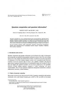
37
Figure 2.1: (a) The Wigner function of the vacuum demonstrates isotropic fluctuations and (b) The Wigner function for the squeezed coherent state given by Eq. (2.49) with α = −2i and σ = 3.0. history, but we use it as a visualization aid only. We choose some simple wave functions and create their Wigner functions. Wigner functions for coherent states and squeezed coherent states have simple expressions. For example, the Wigner function for the vacuum given by Eq. (2.36) is W0 (x, p) =
1 −p2 −x2 , e π
(2.66)
and for the squeezed coherent state given by Eq. (2.49), the Wigner function is Ws (x, p) =
1 −σ2 (p−p0 )2 − (x−x20 )2 σ . e π
(2.67)
Note how neatly the Wigner function simultaneously captures the quadrature variances given by Eqs. (2.51) and (2.52) in Eq. (2.67). The Wigner function for the vacuum is presented in Figure 2.1(a) and for a squeezed coherent state in Figure 2.1(b). For σ = 3.0, the enhanced variance in the x direction and the reduced variance in the p direction is
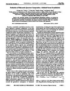
38 clear in Figure 2.1(b). Note that the allowed amount of squeezing of the coherent states of the harmonic oscillator is unbounded. We give an example of a Wigner function that takes on negative values. The sinc function is an orthogonal wave function, which is in L2 (R) and is of interest in our study of continuous-variable quantum algorithms. The sinc function in the position representation is sin(P x) φ(x) = √ , P πx
(2.68)
and its Fourier transform is the momentum top-hat function ⎧ �⎪
⎨ 1, if p ∈ [−P, P ] 1 ˜ φ(p) = √ 2P ⎪ ⎩ 0, if p ∈ / [−P, P ],
(2.69)
having finite extent of 2P in the momentum domain. The Wigner function for the sinc function cannot be simply expressed, so we resort to numerical means to calculate it. In Figure 2.2, we plot the calculated Wigner function for P = 2. In Figure 2.2 (a), we see that quantum interference effects attenuate slowly in the position dimension, whereas they are constrained to P = ±2 in the momentum direction. In Figure 2.2 (b), we demonstrate that this Wigner function takes on negative values. The Wigner function is an ideal tool for studying the coherent states of the harmonic oscillator because it is dependent on the cartesian coordinates x and p it naturally captures the effects of translations and squeezing in the x − p plane. The study of coherent spin states requires visualization of rotations and squeezing, and for this we use spherical Q-functions. For the arbitrary coherent spin state represented as |Ψ� =
�2s k=0
αk |k�, we express
the spherical Q-function [55] as 2s � 2
2s 1
Q(θ, φ) =
k=0
k
sin(θ/2)k cos(θ/2)2s−k αk eikφ .
(2.70)
39
Figure 2.2: (a) The Wigner function the sinc function given by Eq. (2.68). (b) Front elevation view demonstrates negative values. For plotting, we map the cartesian coordinates to the spherical angles as � x �→ sin(θ) cos(φ) 1 + |Q(θ, φ)|2 � y �→ sin(θ) sin(φ) 1 + |Q(θ, φ)|2 � z �→ cos(θ) 1 + |Q(θ, φ)|2 .
(2.71)
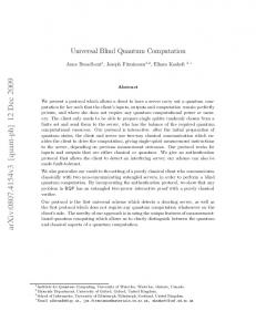
This mapping allows us to represent the quasi-probability distributions on the surface of the unit sphere, which enables an intuitive appreciation for the limits on squeezing in the spin setting. In Figure 5.2(a), we plot the spherical Q-function of continuously-parameterized spin state given by Eq. (5.14). Note that this coherent spin state appears as an ‘equatorial’ state with isotropic uncertainty distribution when represented this way. In Figure 5.2(b), we plot the effect of the squeezing operator given by Eq. (2.62), where μ is such that the Q-function wraps around the equator and ‘touches’ itself. This visually demonstrates why the amount of squeezing is bounded in the spin system case.
40
Figure 2.3: (a) Spherical Q-function of the state given by Eq. (5.14) for s = Squeezed coherent spin state with μ = 0.3.
63 , 2
and (b)
In this section, we have demonstrated that coherent states can be defined for both finite- and infinite dimensional Hilbert spaces having continuous parameterizations. We have shown that coherent states are square-integrable and that they describe physical states, which can be prepared in the laboratory. For these reasons, we will use coherent states in our code-state formalism.
2.4 Spectrum of measurement We operationally define continuous-variable quantum information in terms of continuously parameterized preparation and continuously parameterized measurement, and we define continuous-variable continuously parameterized measurement in terms of the spectrum of an observable. The most general observable is a positive operator-valued measure (POVM) [5]. Projective measurements are employed in this thesis, and projective measurement augmented by unitary operations are equivalent to POVMs [5]. We thus present
41 our discussion on spectrum of measurement in terms of POVMs. A na¨ıve definition of continuous-variable quantum information might be to require the spectrum of the observable in a continuously-parameterized, infinite dimensional system used to process quantum information to consist of real numbers. However, the separability of Hilbert space [50] allows the uncountable basis {|x� ∈ R} to be replaced by a dense countable basis, for example {|q� ∈ Q} with Q the set of rational numbers. Suppose we define the position POVM Px = (|x��x|, x ∈ R) .
(2.72)
The Hilbert space is separable, so there always exists a countable basis. The rational numbers are dense in the reals since every neighbourhood of every real number contains a least one rational number. As a result, we can always define an alternative position POVM Pq = (|q��q|, q ∈ Q) ,
(2.73)
which allows us to construct the countably infinite orthonormal basis �q � |q� = δqq� . The operator Pq is said to be dense in the real numbers. We therefore modify our definition of the measurement spectrum corresponding to continuous-variable quantum information to require that the spectrum of the observable be dense in the reals. We look at how this modified definition of the spectrum of an observable pertains to a continuously-parameterized, finite dimensional system used to process quantum information. Consider the continuously-parameterized phase state [57] of a spin system having dimension 2s + 1 m=s
1 |θ�s = √ eimθ |m�s . 2s + 1 m=−s
(2.74)
For this finite-dimensional Hilbert space, there is no way to construct an observable that is dense in the real numbers.
42 For the interval I ⊂ R, with I = [−π/2, π/2), we can construct the POVM Pθ = (|θ�s �θ|, θ ∈ I) .
(2.75)
However, we can’t have a countably infinite orthonormal basis set for a finite-dimensional Hilbert space, so we can’t construct a POVM whose spectrum is dense in the spectrum of the POVM defined by Eq. (2.75). We thus conclude that a finite-dimensional system is not a continuous-variable quantum information system from the perspective of measurement, but we can still refer to the finite-dimensional case as “continuous variable” from the perspective of preparation. We can use continuous-variable techniques in the analysis of finite-dimensional systems. For example, we can describe a finite-dimensional spin system in terms of continuouslyparameterized spin states [25] and use continuous-variable techniques such as squeezing as we demonstrate in Chapter 5. Indeed this approach of using continuous-variable techniques in finite-dimensional systems is beneficial because it allows us to discover a new quantum algorithm. We continue this background chapter with a discussion of oracledecision problems and algorithms for their solution.
2.5 Oracle-decision Problems The challenge of oracle decision problems is to identify which of two mutually disjoint sets contains a unique N -bit string by making the fewest possible queries to an oracle.
2.5.1 Definition The oracle decision problem is typically couched in terms of a function f that maps n-bit strings to a single bit f : {0, 1}n �→ {0, 1}.
(2.76)
43 Any Boolean function on n bits can also be represented by a string z of N = 2n bits, in which the ith bit zi is the value of the function on the ith bit string, taken in lexicographical order. We use the definition of an oracle decision problem given in [25] as follows. Definition 1. An oracle decision problem is specified by two non-empty, disjoint subsets A, B ⊂ {0, 1}N . Given a string z ∈ A ∪ B = C, the oracle-decision problem is to determine whether z ∈ A or z ∈ B with the fewest queries to the oracle possible. We are interested in finding an efficient strategy to identify the property of whether f belongs to set A or to set B without necessarily determining f itself.
2.5.2 The Deutsch–Jozsa oracle decision problem The Deutsch–Jozsa is a specific example of an oracle-decision problem. The problem is to determine a specific characteristic of an unknown function f : {0, 1}n → {0, 1} of an n-bit input with as few queries as possible. The special characteristic of interest is that the function is guaranteed to be either balanced or constant. We give the definition of the Deutsch–Jozsa problem given in [25] as follows. Problem 1. Given the set of balanced strings A ⊂ {0, 1}N , where exactly N/2 elements take on the value 0 and the set of constant strings B ⊂ {0, 1}N , where all N elements take on the same value everywhere, and a string z randomly selected with uniform distribution μ such that z ∈μ C = A ∪ B, the Deutsch–Jozsa Problem is to determine if z ∈ A or z ∈ B with the fewest oracle queries. Note that the output of a function that is constant has either all 1’s or all 0’s; whereas the output of a function that is balanced has equal number of 1’s and 0’s. For example, for n = 2 the constant functions are {0000, 1111} and the balanced functions are
44 {0011, 0101, 0110, 1001, 1010, 1100}. There are 2N (with N = 2n ) functions in total of �N which 2 are constant and N/2 are balanced.
2.6 Algorithms for solving the Deutsch–Jozsa problem In this section, we present two classical and two quantum approaches to solving the Deutsch–Jozsa problem. In the classical case we, we summarize deterministic and probabilistic algorithms. In the quantum case, we present the traditional discrete quantum algorithm and a two-mode continuous-variable algorithm. Throughout this thesis, we use the integer m to represent the number of queries made to an oracle or the number of times an algorithm is invoked. The best case is where m = 1, and the problem is solved in a single query. If the query complexity is O(m), the solution requires a linear number of queries, and if m = O(N ) then an exponential number of queries is required since N = 2n .
2.6.1 The classical version of the Deutsch–Jozsa algorithm On a classical Turing machine, Problem 1 can be solved deterministically using m = N/2 + 1 queries to determine whether the given function is balanced or constant, with certainty. The problem cannot be solved with certainty with fewer than N/2 + 1 queries because N/2 queries of any balanced function could result in the same value and would thus appear to be a constant function. However, the problem can be solved with much fewer queries by allowing for an incorrect answer with some (small) probability. A probabilistic algorithm achieves an exponentially small error of 2−m with a number of queries that is only linear in m. To understand how a probabilistic algorithm can help, consider that, although a single query with a random input provides no information, two queries with two random inputs can be highly informative. If the output from the second query differs from the first output, then the function is proved not to be constant and
45
H� n
H� n Measurement
Uf X
��0 �
H
��1 �
��2 �
��3 �
��4 �
Figure 2.4: Traditional (n + 1)-qubit discrete-variable circuit implementation of the Deutsch–Jozsa algorithm. The upper line represents the n-qubit ‘control’ state, and the lower line represents the 1-qubit ‘target’ state. therefore must be balanced. If, on the other hand, the second output is the same as the first, then the outcome is not certain, but the more times the outputs are the same, the more confident one can be about the function being constant. We calculate the success probability of determining whether a given function fz is balanced or constant as Pr = 1 − �
�m 1 ≥1− . N − (j − 1) 2
m � N/2 − (j − 1) j=1
(2.77)
Here the equality is calculated assuming randomized input and sampling without replacement and shows dependency on N , whereas the inequality is based on assuming randomized input and sampling with replacement and is independent of N . We note that the failure probability declines exponentially with the number of queries. 2.6.2 The traditional (n + 1) qubit Deutsch–Jozsa algorithm The quantum Deutsch–Jozsa algorithm is an important early quantum algorithm, which demonstrates exponential speed-up over its classical counterpart. The quantum Deutsch–
46 Jozsa algorithm has been shown to solve Problem 1 in a single query [19]. We present a standard circuit version [37] in Figure 2.4. Note that the inclusion of the operator X to create the target state |1� is not the original representation but was given by [37] as � � a means of having the input in the state |Ψ0 � = �0⊗(n+1) . We give a brief and informal analysis of this algorithm here in order to emphasize its salient features. U
0 With reference to Figure 2.4, the first step is to modify the input states |0 · · · 0�|0� −→
|Ψ1 � = |0 · · · 0�|1� through the action of the unitary operator U0 = I⊗n ⊗ X. Note that we will suppress the Kronecker symbol ⊗ when convenient. The next step is to place this state into an equal superposition of all computational basis states ⎛ ⎞
1 U1 |Ψ1 � −→ |Ψ2 � = ⎝ √ |x�⎠ |−� 2n x∈{0,1}n
(2.78)
through the action of the operator U1 = H⊗n ⊗ H. The placing of the target qubit into the state |−� is critical since as we shall see, this clever arrangement serves to ‘kick back’ the phase of the oracle function to the control state superposition. Uf
The crucial step, is to apply the oracle function to transform |Ψ2 � −→ |Ψ3 � The oracle construct originally proposed by Deutsch–Jozsa is expressed, for x ∈ {0, 1}n and y ∈ {0, 1}, as Uf : |x�|y� �→ |x�|y ⊕ f (x)�.
(2.79)
With this definition of the oracle, the state |Ψ3 � may be represented as follows � �
|0 ⊕ f (0 · · · 0)� − |1 ⊕ f (0 · · · 0)� 1 √ |0 · · · 0� |Ψ3 � = √ 2n 2 �
|0 ⊕ f (0 · · · 1)� − |1 ⊕ f (0 · · · 1)� √ +|0 · · · 1� 2 �
|0 ⊕ f (1 · · · 0)� − |1 ⊕ f (1 · · · 0)� √ + · · · + |1 · · · 0� 2 ��
|0 ⊕ f (1 · · · 1)� − |1 ⊕ f (1 · · · 1)� √ . +|1 · · · 1� 2
(2.80)
47 The function f (x) can only take on the values 0 and 1. When f (x) = 0, the phase of the target qubit |−� =
√1 2
(|0� − |1�) in the above expression remains unchanged, but when
f (x) = 1, the phase of |−� is flipped. Since flipping the phase is equivalent to multiplying the target state |−� by −1, we can rewrite Eq. (2.80) as follows 1 � |Ψ3 � = √ (−1)f (0...0) |0 . . . 0� + (−1)f (0...1) |0 . . . 1�+ n 2 . . . + (−1)f (1...0) |1 . . . 0� + (−1)f (1...1) |1 . . . 1�
� |0� − |1� √ 2 ⎞ ⎛
1 (−1)f (x) |x�⎠ |−�. = ⎝√ n 2 x∈{0,1}n
(2.81)
Note that the appearance of the term (−1)f (x) multiplying each component of the control state superposition is what we term phase ‘kick back’. The result expressed in Eq. (2.81) means that the oracle definition given in Eq. (2.79) may be equivalently expressed as Uf : |x�|y� �→ (−1)f (x) |x�|y�,
(2.82)
which is a convenient representation for comparison to the oracle implemented in an n-qubit algorithm. This is a demonstration of how the quantum advantage is achieved by exploiting the superposition of all computational basis states. In the penultimate step, we focus on the control portion only as the target remains unchanged. We express the control portion of the final state as the action of H⊗n on |Ψ4c � as follows ⎛ ⎜ ⎜ 1 ⎜ ⎜ |Ψ4c � = n ⎜ 2 ⎜ ⎜ ⎝
1
1 ···
⎞⎛ 1
1 −1 · · · −1 .. .. . . .. . . . . 1 −1 · · ·
1
⎞ (−1)f (0···0)
⎟⎜ ⎟⎜ ⎟ ⎜ (−1)f (0···1) ⎟⎜ ⎟⎜ .. ⎟⎜ . ⎟⎜ ⎠⎝ (−1)f (1···0)
⎟ ⎟ ⎟ ⎟ ⎟. ⎟ ⎟ ⎠
(2.83)
48 For the two constant cases, we have ⎛ ⎜ ⎜ ⎜ � ++ � 1 ⎜ �Ψ4c = ± n⎜ 2 ⎜ ⎜ ⎝
1
1 ···
⎞⎛ 1
1 −1 · · · −1 .. .. . . .. . . . . 1 −1 · · ·
1
⎞
⎛
1
⎟⎜ ⎟ ⎜ ⎟⎜ ⎟ ⎜ ⎟⎜ 1 ⎟ ⎜ ⎟⎜ ⎟ ⎜ ⎟⎜ ⎟ = ±⎜ ⎟⎜ ⎟ ⎜ ⎟⎜ 1 ⎟ ⎜ ⎠⎝ ⎠ ⎝ 1
⎞ 1 0 .. .
⎟ ⎟ ⎟ ⎟ ⎟, ⎟ ⎟ ⎠
(2.84)
0
where the symbol ++ denotes a constant string. The last step in Eq. (2.84) is true since all the rows of H⊗n have an equal number of plus 1’s and minus 1’s except for the first, which results in all amplitudes of the components of the final control state being zero except for the first. We now consider one of the balanced cases as a point of illustration. For the case where f = 0101 · · · 01, we can simply express the result as follows ⎛ ⎜ ⎜ ⎜ � +− � 1 ⎜ �Ψ4c = n⎜ 2 ⎜ ⎜ ⎝
1
1 ···
⎞⎛ 1
1 −1 · · · −1 .. .. .. . . . . . . 1 −1 · · ·
1
⎞
⎛
⎞
1 0 ⎟⎜ ⎟ ⎜ ⎟ ⎟⎜ ⎟ ⎜ ⎟ ⎟ ⎜ −1 ⎟ ⎜ 1 ⎟ ⎟⎜ ⎟ ⎜ ⎟ ⎟⎜ . ⎟ = ⎜ . ⎟, ⎟⎜ . ⎟ ⎜ . ⎟ ⎟⎜ . ⎟ ⎜ . ⎟ ⎠⎝ ⎠ ⎝ ⎠ −1 0
(2.85)
where the symbol +− denotes a balanced string. The last step in Eq. (2.85) is true since only the second row of H⊗n has an alternating number of plus 1’s and minus 1’s, which results in all amplitudes of the components of final control state being zero except for the second. Since all balanced functions result in � � a state �Ψ+− having and an equal number of plus 1’s and minus 1’s, the first component 4c of the amplitude is always zero. The non-zero value will land on the component that corresponds to the row in H⊗n that matches the phase of the balanced function. The final step is to make a projective measurement [5] on the first qubit. If the measurement returns a one, the unknown function is constant, and if the measurement returns a zero, the unknown function is balanced. This analysis demonstrates that the
49
�
�† Measurement
Uf �
��0 �
��1 �
��2 �
��3 �
Figure 2.5: Two-mode continuous-variable circuit implementation of the Deutsch–Jozsa algorithm uses two oscillator modes [18]. The upper line represents the ‘control’ position state, and the lower line represents the ‘target’ position state. traditional discrete-variable Deutsch–Jozsa algorithm solves this problem in a single query by relying on an oracle that kicks-back the phase of the function thus exploiting the quantum advantage. In the next, and final subsection of this background chapter, we study an attempt to directly map this version of the discrete quantum algorithm to the continuous-variable setting.
2.6.3 The two-mode continuous-variable Deutsch–Jozsa algorithm The circuit shown in Figure 2.5 depicts the continuous-variable Deutsch–Jozsa algorithm given in [18]. This algorithm uses two separate modes of the harmonic oscillator, which are represented by the horizontal lines in the figure. The top line is the position eigenstate |x0 �, which corresponds to the n-qubit control state in the traditional discrete algorithm, and the bottom line is the position eigenstate |π�, which corresponds to the 1-qubit target state in the traditional discrete algorithm shown in Figure 2.4. Both the control and the target states are defined to meet the Dirac orthogonality condition �x|x� � = δ(x − x� )
50 given in Eq. (2.15). The steps of the algorithm are analogous to the steps of the discrete algorithm. The input state |x0 �|π� is transformed into a superposition by applying the continuous Fourier transform. The superposition is expressed as 1 F|x0 �F|π� = √ 2π
� dx dy eix0 x+iπy |x�|y�.
(2.86)
Note that we have changed the definition of the Fourier transform given in [18] to the standard transform [56] given in Eq. (2.27) for consistency with [20, 24]. With this definition, the target state is |π� instead of |π/2� used in [18]. The oracle mapping is the continuous-variable analogue of the discrete mapping given in Eq. (2.79) Uf : |x�|y� �→ |x�|y + f (x)�,
(2.87)
where the + sign is the continuous-variable equivalent of the XOR function [9]. The action of the oracle on the superposition state given by Eq. (2.86) is � 1 dx dy eix0 x+iπy |x�|y + f (x)� Uf (F|x0 �F|π�) = √ 2π � 1 =√ dx dy eix0 x eiπy+iπf (x) |x�|y� 2π
� � 1 ix0 x f (x) = √ dx e (−1) |x� F|π�. 2π
(2.88)
We have been careful in the preceding to show that the algorithm was designed to mimic the phase kick-back employed in the traditional discrete quantum algorithm. In particular setting the target position state to |π� achieves the desired effect since eiπf (x) = (−1)f (x) . The state after the inverse Fourier transform is given by †
F [ Uf (F|x0 �F|π�)] =
�
�
dxdx� eiπ(x0 −x ) (−1)f (x) |x� �F|π�.
(2.89)
51 Measurement is achieved by projecting this resultant state onto the original state using the idealized continuous-variable projection operator [18]. � PΔx0 =
x0 +Δx0 /2
dy|y��y|.
(2.90)
x0 −Δx0 /2
Note that this measurement has finite spread Δx0 . The balanced and constant argument is then made. The essence of the argument is that if the function is constant, the state given by Eq. (2.89) is simply ±|x0 �|π� and the measurement returns one. If the function is balanced then the output is orthogonal to the constant case and measurement returns zero [18]. The result of this analysis is the claim [18] that the reduction in the number of query calls is from infinity to one, but there are fundamental issues that make this a false conclusion. These issues all stem from the fact that infinitesimal position states are employed as the computational basis, and these states do not meet the square-integrable condition given by Eq. (2.28). Encoding the oracle information into proper squareintegrable basis states changes this conclusion [20].
2.7 Summary In this chapter, we have presented a comparison of the quantum advantage in both the discrete and continuous quantum settings. The maximum state overlap is analogous in the two settings, but the continuous form allows for the potential for ill-defined position states. Our code-state formalism requires square-integrable functions in L2 (R). Any functions that meet the square-integrable and Fourier-transform pair requirements can be used. Orthogonal wave functions have features that can be beneficially exploited. Coherent states of the harmonic oscillator and coherent spin states also both meet the square-integrable requirements. Coherent states are over-complete and therefore are said to be non-orthogonal. Coherent states are particularly attractive because they can
52 be created in the laboratory, and there is a collection of tools that can realize most of the algorithm components. Implementation of the oracle remains the biggest challenge. Oracle decision problems are defined, and algorithms for the solution of the Deutsch– Jozsa oracle decision problem are presented. The traditional quantum algorithm exploits quantum parallelism and solves the problem in a single query. An attempt to map the traditional quantum algorithm to a continuous-variable setting using two modes of the oscillator draws false conclusions because of the use of improper, non-renormalizable states. In the next chapter we introduce a code-state formalism employing orthogonal wave functions in L2 (R), which enables the correct analysis of algorithm performance.
53
Chapter 3 CONTINUOUS-VARIABLE QUANTUM COMPUTATION WITH ORTHOGONAL STATES 3.1 Introduction In continuous-variable quantum information procedures, the input state is typically a Gaussian wave function over the canonical position representation with the physical system being a harmonic oscillator (equivalently a single-mode optical field [46]). However, the unbounded extent of these wave functions does not naturally fit with the finite length of the information strings being processed. To deal with the problem of finite-length information strings, we first develop our code-state formalism using orthogonal wave functions [20]. In this chapter, we focus on a continuous-variable generalization of the Deutsch–Jozsa algorithm to the case of a single mode of light. To deal with the single mode of light, we first introduce a variation of the traditional discrete-variable Deutsch–Jozsa algorithm that employs only n qubits. We then map this algorithm into the continuous-variable setting using a single mode of light and a Fourier transform performing the equivalent of the Hadamard transformation. There are three advantages in working with this approach. One is that Braunstein and Pati [18] introduced a two-mode continuous-variable Deutsch–Jozsa algorithm, which we analyzed in Sec. 2.6.3. We can learn from their approach of requiring infinitesimal position states. The second advantage is that the single mode continuous-variable Deutsch–Jozsa algorithm employs standard quantum optics techniques. The third advantage is that we can demonstrate how the Fourier transform is itself responsible for the limitations of
54 continuous-variable schemes. This chapter is organized as follows. In Sec. 3.2, we introduce a recasting of the traditional Deutsch–Jozsa algorithm from an (n + 1)-qubit algorithm to an n-qubit algorithm, which does not employ the target qubit. In Sec. 3.3, we motivate the selection of the continuous-variable model and introduce techniques for bounding the success probability. In Sec. 3.4, we calculate the single-query success probability Pr⊥ � and bound the query complexity after m repetitions. We summarize in Sec. 3.5.
3.2 An n-qubit quantum Deutsch–Jozsa algorithm The quantum Deutsch–Jozsa algorithm has been shown to solve Problem 1 in a single query [19]. We presented an analysis of the traditional algorithm in Sec. 2.6.2 using the standard circuit version [37] presented in Figure 2.4. This standard circuit employs n + 1 qubits. The extra qubit is referred to as the target qubit and is represented by the lower line in Figure 2.4. In order for easier adaption of this circuit to the continuous-variable setting, we choose an alternative, and equivalent, circuit formulation — one without the target state. We take this approach because the n-qubit model can be implemented in single mode of the harmonic oscillator rather than the two-mode model employed in [9]. The unitary operator associated with the oracle function changes slightly in this alternative circuit. This simpler algorithm without the target qubit is given in Figure 3.1. In Chapter 2, we demonstrated that the oracle construct originally proposed by Deutsch–Jozsa and given in Eq. (2.79), may be equivalently expressed as Uf : |x�|y� �→ (−1)f (x) |x�|y�,
(3.1)
which is given in Eq. (2.82) and is re-expressed here for ease of reference. This construction yields a matrix representation for Uf as a permutation matrix, hence always
55
�
H� n
H� n
Uf
Measurement
�
�
��0 �
��1 �
�
��2 �
�
��3 �
Figure 3.1: Alternative n-qubit discrete-variable circuit implementation of the Deutsch–Jozsa algorithm. Note the absence of the target qubit and the use of the operˆ f defined in Eq. (3.3) ator U unitary [5]. The representation of the oracle given in Eq. (3.1) demonstrates that the target qubit remains unchanged and that it only provides a mechanism to encode the j th bit of the unknown oracle string into the phase of the j th computational basis state comprising the control state. With respect to the ordered basis B = {|0 · · · 0�|0�, |0 · · · 0�|1�, . . . , |1 · · · 1�|0�, |1 · · · 1�|1�} , the unitary matrix Uf can be expressed in the following insightful form ⎞ ⎛ f (0···0) 0 ··· 0 X ⎟ ⎜ ⎟ ⎜ f (0···1) ⎟ ⎜ 0 X · · · 0 ⎟ ⎜ Uf = ⎜ ⎟, .. .. .. ... ⎟ ⎜ . . . ⎟ ⎜ ⎠ ⎝ f (1···1) 0 0 ··· X
(3.2)
with X the 2 × 2 NOT operator in this case. The operator Uf can also be expressed in the alternative ordered basis with |+� = √1 2
(|1� + |0�), |−� =
√1 2
(|1� − |0�) and
B � = {|0 · · · 0�|−�, |0 · · · 1�|−�, . . . , |1 · · · 0�|+�, |1 · · · 1�|+�} ,
56 as
⎞ ˆ ⎜ Uf 0 ⎟ Uf = ⎝ ⎠, 0 11 ⎛
ˆ f is expressed as the with 11 the 2n × 2n identity operator. Furthermore the operator U 2n × 2n matrix
⎛ ⎜ ⎜ ⎜ ˆf = ⎜ U ⎜ ⎜ ⎜ ⎝
(−1)f (0···0) 0 .. .
···
0
f (0···1)
.. .
··· ...
0 .. .
0
· · · (−1)f (1···1)
(−1)
0
⎞
0
⎟ ⎟ ⎟ ⎟ ⎟, ⎟ ⎟ ⎠
(3.3)
and thus provides a reduced representation for Uf . It is clear from the matrix represenˆ f that the oracle construct for Uˆf is simply tation of U Uˆf : |x� �→ (−1)f (x) |x�,
(3.4)
where we note the absence of the target qubit that appears in Eq. (3.4). ˆ f acts non-trivially only on a 2n -dimensional subIt is apparent that the operator U space of the 2n+1 -dimensional space. This correspondence is clear in the following identity relation � � � � ˆ f ⊗ |−��−| ⊕ 11⊗n ⊗ |+��+| . Uf = U ˆf. Thus, there is an equivalence between employing the oracle Uf , or its counterpart U Oracle equivalence can also be understood because one of the oracles can be used to simulate the other [37]. We conclude that the construction employing both control and target qubits is not strictly necessary. We now present a step-by-step analysis of the alternative circuit presented in Figure 3.1. We shall analyze the continuous-variable circuit in the same steps for cross ˜ j � in order to emphasize that reference and comparison. We use the tilde notation |Ψ
57 this analysis is of the algorithm presented in Figure 3.1. The n qubit input state of this ˜ 0 � = |0 · · · 0�. We place this state into an equal circuit is a string of qubits prepared in |Ψ superposition of all computational basis states ˜ 0 � �→ |Ψ ˜ 1 � = 2−n/2 H⊗n |Ψ
|x�
x∈{0,1}n
for H the single qubit Hadamard operator. ˆ f defined in Eq. (3.3), its effect on the Given the definition of the reduced operator U ˜ 1 � is to encode the N -bit equal superposition of basis states expressed in the state |Ψ ˜ 2 �. We express this as string z unitarily into the state |Ψ ⎛
⎞ f (0···0)
(−1) ⎜ ⎟ ⎜ ⎟ ⎜(−1)f (0···1) ⎟ ⎟ ˆ f |Ψ ˜ 1 � �→ |Ψ ˜ 2 � = 2−n/2 ⎜ U ⎜ ⎟, . ⎜ ⎟ .. ⎜ ⎟ ⎝ ⎠ f (1···1) (−1)
(3.5)
which is a convenient representation. We shall show that this representation naturally extends to the continuous-variable setting. Measurement proceeds by first undoing the superposition created during the state preparation step. The resultant state may be expressed as follows ⎛
⎞⎛
⎞
1 1 ··· 1 (−1) ⎜ ⎟⎜ ⎟ ⎟⎜ ⎜ ⎟ f (0···1) ⎟ ⎟ ⎜ ⎜ (−1) 1 −1 · · · −1 ⎟⎜ ⎟ ˜ 3� = 1 ⎜ |Ψ ⎜. . ⎟⎜ ⎟. n . . ⎟ 2 ⎜. . ... . ⎟ ⎜ .. . ⎟⎜ ⎜. . ⎟ ⎝ ⎠⎝ ⎠ f (1···1) 1 −1 · · · 1 (−1) f (0···0)
(3.6)
Eq. (3.6) allows us to see that all of the rows (and columns) of the operator H⊗n have an equal number of positive and negative ones except for the first row, which consists entirely of plus ones. It is this feature that permits the constant and balanced functions to be distinguished in a single measurement.
58 ˜ 3C � = ±(10 · · · 0)� as For the two constant cases, Eq. (3.6) results in the state |Ψ only the first row does not result in amplitude cancellation of the 2n constant amplitude ˜ 2 �. Each of the balanced functions result in the amplitudes components of the state |Ψ ˜ 2 � having an equal number of positive and negative ones. This feature of the state |Ψ ˜ 3 � having zero amplitude for all the balanced results in the first component of the state |Ψ ˜ 3B � = ±(0 x · · · x)� where we use the symbol x to functions. We express this result as |Ψ represent the non-zero value(s) that land on the other N − 1 components depending on �N balanced functions the oracle is set to. which of the N/2 For the final measurement step, we employ the projection operator [5] defined for m ∈ {0, 1}N as follows Mm = |m��m|.
(3.7)
We are only concerned with the first component as discussed above, so for the constant cases we have
� � � � �˜ ˜ Pr[m = (0 · · · 0)] = Ψ3C � M(0···0) �Ψ3C = 1, �
(3.8)
and for all balanced cases we have � � � � �˜ ˜ Pr[m = (0 · · · 0)] = Ψ3B � M(0···0) �Ψ3B = 0 �
(3.9)
as required. We have established that the n-qubit discrete Deutsch–Jozsa algorithm gives the same result as the standard implementation. In the next section we formulate how to adapt the n-qubit model to the continuous-variable setting.
3.3 Single mode continuous-variable algorithm with orthogonal states There are many potential models representing continuous-variable Deutsch–Jozsa algorithms. Both single-mode and multiple-mode models can be analyzed; each model can
59 be studied using input states represented by different L2 (R) functions; also different oracle encoding schemes can be envisaged. In this section, we present the arguments for studying a particular one-mode model that offers insight into the key features of all continuous-variable models.
3.3.1 Continuous-variable model selection Our strategy is to create a model of the continuous-variable Deutsch–Jozsa algorithm that naturally relates to the discrete case, employs reasonable resources, is generally applicable and is independent of particular basis functions. Discrete quantum information algorithms solving oracle decision problems follow a pattern: prepare the input state in one of n computational basis states ∈ Cn ; apply the Hadamard transformation to place the input state in an equal superposition of basis states; apply a unitary operator representing the oracle; undo the superposition by again applying the Hadamard operator, and perform a projective measurement of a particular basis state. The probability of the desired outcome is the square of the magnitude of the amplitude of the particular basis state. In order for our continuous-variable model to relate naturally to the discrete case, we mimic this pattern using the position and momentum states of a single particle. We choose a single-mode continuous-variable model for the following reasons. First, we can apply the necessary algorithm features with minimal resources using the tools of quantum optics. Second, this single mode has infinite dimension, which is intrinsically more than sufficient to solve the problem. If it cannot be solved in a single-mode model, it is highly desirable to gain insight into the fundamental reasons why not. Third, Braunstein and Pati’s techniques [18] employ a similar model that although it is a two-mode model employing a continuous-variable target state, the results of our single-mode model are directly applicable to it.
60
fz�N�� p�
F
F� Measurement
Φ0 �x�
� Φ�p�
� �N� Φz �p�
Φ�N� z �x�
Figure 3.2: Single mode continuous-variable quantum circuit implementation of the Deutsch–Jozsa algorithm without the use of the target state. F is the continuous (N ) Fourier transform given by Eq. (3.12) and fz (p) is the oracle encoding function given by Eq. (3.20). Our algorithm is the continuous-variable analogue of the alternative formulation of the discrete Deutsch–Jozsa algorithm presented in Figure 3.1. We present the continuousvariable version of this algorithm in Figure 3.2. In our model, we also choose to encode the strings z ∈ {0, 1}N into an orthogonal basis of square-integrable complex-valued functions over the reals, namely L2 (R). Since information is of finite length and can be represented by N -bits, it is desirable that the encoded functions form a compact basis with p ∈ [−P, P ]. We address the problem of encoding finite information into the nonorthogonal and non-compact Gaussian states in Chapter 4.. To deal with the problem of finite-length information strings, we encode the information into a finite region of the momentum domain. Information is represented by finite-length bit strings z ∈ {0, 1}N with N the number of bits. These strings are encoded into a region of the momentum domain p extending from -P to P . A regular lattice of N discrete values of p are embedded in this domain such that the ith bit of z, is assigned to p as follows: pzi := (1 + 2i − N ± 1)P/N . The lattice is thus {pzi } with spacing 2P/N .
61 An orthogonal basis of top-hat functions is formed from the pzi , and the encoded �N −1 momentum wave function is expressed as √12P i=0 (−1)zi |pzi �. The kets |pzi � are phasemodulated by their corresponding bit values, and with this phase modulation, each of the possible 2N strings is uniquely represented. Note that the constant wave function is the top-hat function extending from −P to P . There is a translational invariance between computational basis states because each of the top-hat basis functions occupies an identically-sized region of momentum space and because the string z � is obtained from the string z by the translation z � = z ⊕ (z ⊕ z � ). We can regard this finite basis as an infinite basis modulated by a top-hat function extending from −P to P , which has the effect of truncating the allowed strings from an infinite domain to being from 0 to N − 1. We select x, p ∈ R and use the particle’s position wave function, φ(x) to describe both the input and output states. The information representing the oracle is encoded ˜ into the momentum wave function φ(p). The position and momentum wave functions are Fourier transform pairs, and the relationship between the particle’s position and its momentum is governed by Heisenberg’s uncertainty principle. We selected x and p for illustrative purposes and use it throughout for convenience. We note however that it is unimportant in principle whether information is encoded in x or p — or indeed anything in between. Regarding the use of the continuous Fourier transform we note that in the oracle setting, any mathematically-allowed transformation is indeed permitted for the oracle, but the non-oracle operations should be described in an implementable way. Thus, we choose a transformation that is amenable to current or planned technology. It is germane to our scheme that the canonical position and momentum bases are dual to each other in the sense that the Fourier transform is the analogue of the Hadamard transformation for qubit-based quantum computation. We thus exclude the use of the discrete Fourier
62 or Hadamard transformations in this model. Our approach to the creation of a single-mode continuous-variable Deutsch–Jozsa algorithm differs from that of Braunstein and Pati [18] in two key areas. First, our approach relies only on states that are elements in the Hilbert space congruent to L2 (R). Second, our approach does not require the use of the target state. Although their model employs the target state, it only serves to ‘kick back’ the phase of the oracle function and the conclusions from both models should be identical. The basic algorithm elements required to implement the single-mode continuousvariable model are input state preparation; Fourier transform; oracle application and measurement. Our model requires that the momentum wave function be compact and the encoding be unambiguous. We define the following function, along with its Fourier dual, to help us achieve this end. For P > 0, the ‘top hat’ function �(p; P, P0 ) = �p| � (P, P0 )� ⎧ ⎪ 1 ⎨ 1, if p ∈ [P0 − P, P0 + P ] =√ , 2P ⎪ ⎩ 0, if p ∈ / [P0 − P, P0 + P ]
(3.10)
has the compact feature. We also note that lim |� (p; P, P0 )|2 = δ(p − P0 ),
P →0
(3.11)
so the state |�� is, in some sense, a momentum eigenstate |p = P0 � in the limit P → 0. The state given by Eq. (3.10) is the Fourier transform of the desired input state. Here the Fourier transform acts as the continuous version of the discrete Hadamard transform (extending the Hadamard transformation to the continuous-variable case is not unique [21, 57]). For x the canonical position and p the canonical momentum, the ˜ Fourier transform maps a function φ(x) to its dual φ(p) according to [56] ˜ F : φ(x) �→ φ(p),
(3.12)
63 such that ˜ = √1 φ(p) 2π and 1 φ(x) = √ 2π
�
∞
dx eipx φ(x),
−∞
�
∞
˜ dp e−ipx φ(p).
−∞
Note that φ(x) = �x|φ�; the momentum state |p� is the Fourier transform of |x�, and ˜ = �p|φ�. φ(p) The inverse Fourier transform of the function eix0 � (p; P, P0 ) gives the input state, which is described by the sinc function φ(x) =�x|φ� =
eiP0 sin (P (x − x0 )) √ P π(x − x0 )
(3.13)
centred at x0 . The limit of |φ(x)|2 as P goes to ∞ yields δ(x−x0 ). The position eigenstate |x = x0 � is likewise formed in the limit P → ∞. Our model of the oracle encodes the N -bit string z into the compact domain [−P, P ]. Since each of the N -bits comprising the string is represented unambiguously, the contiguous momentum pulses within [−P, P ] have width δp = 2P/N , and for j ∈ {0, N − 1}, the j th momentum pulse is centred at position −P + (j + 1/2)δp and takes on value (−1)zj . The oracle can be repressed in Dirac notation as UCV : |pj � �→ (−1)zj |pj �,
(3.14)
ˆ f given in Eq. (3.4). We illustrate this which is equivalent to the oracle construct for U oracle behaviour in Figure 3.3 for a particular N = 4 balanced case. Note that each of the unique balanced and constant strings form a set of orthogonal functions ∈ L2 (R) when encoded in this manner. The final quantum element of our algorithm is measurement. We measure finite intervals of the probability density function |φi (x)|2 , with the index i representing the
64
z0 �0
z2 �0
P �P z1 �1
p
z3 �1
Figure 3.3: Illustration of the concept for encoding an N -bit string in a region of momentum extending from −P to +P using the N = 4, z = 0101 example. Note that each of the bits zj are uniquely represented by individual pulses of height ± √12P , width δp = 2P/N centred at −P + (j + 1/2)δp . encoded function. This is preferable to making precise measurements of real numbers. The continuous-variable analog of the projection operator given in Eq. (3.7) is defined as � Eab
a
=
|x��x|dx,
(3.15)
b
and thus the probability of detecting the wave function φi (x) in the interval [a, b] is �
a
Pr[φi ] =
|φi (x)|2 dx.
(3.16)
b
With these concepts in order, we illustrate the four stages of our algorithm in Figure 3.4. We begin with the position wave function centered at x0 = 0 and illustrated in Figure 3.4(a). In Figure 3.4(b), we present the momentum wave function, which acts as the ‘substrate’ into which the N -bit strings are encoded. In Figure 3.4(c), the compact pulse function is encoded with the particular N -bit string z = {0 · · · 01 · · · 1}. Finally, the inverse Fourier transform of this ‘square wave’ is presented in Figure 3.4(d). Since
65
P
1
Π
2�P �a�
2�Π �P
x
2�Π P
0
�b�
�P
2�P
�1
p
P
P
1
�P
0
Π �Δ
�c� P
2�P
Δ
�d�
p
2�Π �P
0
2�Π P
x
Figure 3.4: Overview of the four stages of our continuous-variable Deutsch–Jozsa algorithm: (a) The probability distribution of the input state. (b) The Fourier transform of the position state acts as the encoding ‘substrate’. (c) The N -bit string z = {0 · · · 01 · · · 1} modulates this ‘substrate’. (d) The inverse Fourier transform of the encoded ‘square wave’ necessitates an optimal measurement ‘window’ parameterized by ±δ. the inverse Fourier transforms of finite pulses in the momentum domain have infinite extent in the position domain, we need to limit the extent of our measurement to ±δ. We briefly summarize the key features of our single-mode model of the Deutsch–Jozsa algorithm. Our continuous-variable Deutsch–Jozsa algorithm requires the parameters N , which represents the size of the problem, the momentum ‘length’ P over which the information is encoded, and the extent of the measurement window, δ. Since the Fourier transform maps compact states into non-compact states, we expect to determine relationships between these parameters.
66 3.3.2 Encoding Information into Orthogonal States In this subsection, we analyze the single-mode continuous-variable Deutsch–Jozsa algorithm presented in Figure 3.2. This algorithm employs position states represented by sinc functions; employs the continuous Fourier transform; has oracle-encoded states represented by modulated top-hat functions, and employs the continuous-variable projection operator. We show that this model results in an uncertainty principle between the momentum ‘length’ P over which the N -bit string is encoded and the position ‘length’ δ corresponding to the optimum measurement window. This uncertainty implies that this model results in an algorithm that is necessarily probabilistic. We argued previously that we need the Fourier transform of the input state to be the top hat function defined in Eq. (3.10). We add several conditions that do not take away from the generality of the solution. First, we want the top hat to have zero phase, which gives x0 = 0 and to be centred at P0 = 0. Second, we want the pulse to have extent ±P . This gives us the simplest form of the sinc function for the initial state sin(P x) . φ0 (x) = √ πP x
(3.17)
With reference to Figure 3.2, the next step in the algorithm is to perform the Fourier transform, which yields the top hat function with extent ±P ⎧ ⎪ ⎨ 1, if p ∈ [−P, P ] 1 ˜ =√ φ(p) 2P ⎪ ⎩ 0, if p ∈ / [−P, P ].
(3.18)
This function forms the raw substrate, which is ‘modulated’ by the individual N -bit strings z. We perform encoding by partitioning the real numbers representing momentum into non-overlapping, contiguous and equal-sized bins. In this digital-to-analogue strategy,
67 the width of each p-bin is 2P/N , and ⎧ � � � ⎪ ⎨ 1, p ∈ − 1 − 2 N −1−i , − 1 − 2 N −i P N N (N ) �i (p) = ⎪ ⎩ 0, otherwise.
(3.19)
The oracle encodes the index z into the function fz as follows: fz(N ) (p)
=
N −1
(N )
(−1)zi �i
(p),
(3.20)
i=0
where the factor (−1)zi serves to modulate the phase of the top hat function according to the bit value. Example 1. Consider the case n = 2; hence N = 22 = 4. As one case, the function corresponding to the four-bit string 0011 is (N )
(N )
(N )
(N )
(N )
f0011 (p) = �0 (p) + �1 (p) − �2 (p) − �3 (p).
(3.21)
The only two four-bit strings yielding constant functions would be 0000, for which the function is identically unity over the whole domain [−P, P ], and 1111, for which the function is identically −1 over [−P, P ]. Four cases are presented in Figure 3.5. In the limit that N → ∞ with P fixed, | �i (p)|2 �→ δ(p − pi ) for pi the midpoint of the ith bin. The limit N → ∞ thus gives a prescription for approaching a continuous variable representation where the z index seems to approach a continuum; however this limit yields a countable, rather than uncountable, set {z}, and the finite domain [−P, P ] has important ramifications on the nature of the functions corresponding to Fourier transforms of �i (p). We express the state after encoding as ) (N ) ˜ φ˜(N (p)φ(p), z (p) = fz
(3.22)
where we observe the ‘modulating’ effect of the encoded string fz on the momentum ˜ ‘substrate’ φ(p).
68
1
1 �a�
�b� 1
�1 �1
0
�1
1 1
1
�c�
�d�
1 �1
�1 �1
1 �1
(4)
Figure 3.5: Encoded functions fz (p) (a) z = 0000, (b) z = 0011,(c) z = 0101, and (d) z = 0110. We have the strings z ∈ {0, 1}N encoded into the momentum state (3.22). The next step is to take the inverse Fourier transform of this pulse train. For zj the j th bit of z, this is expressed as sin(P x/N )
= √ (−1)zj eiϕj (x) , P π x j=1 N
) φ(N z (x)
� where we have set ϕj (x) =
(2j−1)−N N
(3.23)
� P x. We see that the magnitude of an individual
(N )
generalized sinc function, φz (x), is determined by a vector sum of N phasors, which is modulated by a particular N -bit string z. The phasors, eiϕj (x) , are equiangular divisions of the angular interval [−(N − 1)P x/N, (N − 1)P x/N ], and they exhibit the pairwise complex conjugate property ϕj (x) = −ϕN +1−j (x). In Figure 3.6, we present the phasors for N = 8 with P x = π/2 and P x = π/4 to illustrate these features. (N )
We note that the only functions with φz (0) �= 0 are the two constant sinc functions.
69
0.08
0.08
�a�
0
�b�
0
0.08
�0.08
0.08
�0.08
Figure 3.6: The phasors eiϕj x defined in Eq. (3.23) for N = 8 (a) P x = π/2 phasors range between ±7π/16 in steps of π/8, and(b) P x = π/4 phasors range between ±7π/32 in steps of π/16. � zj = ±N for the two constant cases, and N j=1 (−1) = �N 0 for all balanced cases. This feature of the set of N/2 + 2 sinc functions represented
This is clear given that
�N
j=1 (−1)
zj
(N )
by φz (x) implies that the strategy for measurement that distinguishes between the constant and balanced cases is to measure about x0 = 0. We measure the probability distribution in a small band around the position x0 = 0. Due to the symmetry of the sinc functions about x0 , we employ the continuous-variable projection operator given in Eq. (3.15) and set a = δ and b = −δ. The probability of detecting a particular wave function in the interval ±δ is thus expressed as Pr
�
� ) φ(N z (x)
δ
= −δ
� (N ) �2 �φz (x)� dx.
(3.24)
We now need to determine the optimal value of measurement window δ that maximizes
70 our ability to distinguish between the constant and balanced cases.
3.4 Bounding the success probability We first determine which of the balanced functions dominates the region ±δ and set bounds on the value of δ. We hypothesize that the dominant balanced functions are the balanced functions having the lowest ‘frequency’ content. This occurs when the first N/2 bits and the last N/2 bits have opposite values. For this pair of balanced functions, which we call the antisymmetric balanced (AB) functions, we have ⎧ ⎫ ⎨ ⎬ AB ∈ 0! ·"# · · 0$ 1! ·"# · · 1$, 1! ·"# · · 1$ 0! ·"# · · 0$ . ⎩ ⎭ N/2
Note that of the
�
N N/2
N/2
N/2
(3.25)
N/2
balanced functions, there are many that are also antisymmet-
ric about the midpoint. However, we reserve the term AB for these two lowest-order antisymmetric balanced functions. Before proving the antisymmetric balanced function dominates all other balanced functions in the region ±δ, we illustrate the concept of frequency in the following example. Example 2. Again consider the case P = 1, n = 2; hence N = 22 = 4. As one case, the function corresponding to the four-bit string 0011 is (4)
� x x 3x sin(x/4) � −i 3x √ e 4 + e−i 4 − ei 4 − ei 4 πx i (cos x − 1) √ = πx
φ0011 (x) =
(3.26)
This function corresponds to the N = 4 antisymmetric balanced function. The probability distributions for the four distinct N = 4 cases are presented in Figure 3.7. We clearly see that of the three balanced cases, the N = 4 antisymmetric balanced function has probability peaks closest to x0 = 0 and thus has the lowest frequency content.
71
0.35
0.35
�a�
�10
�5
0
5
�b�
10
�10
�5
0
0.35
�5
10
0.35
�c�
�10
5
0
5
�d�
10
�10
�5
0
5
10
(4)
Figure 3.7: The probability distributions |φz (x)|2 for (a) z = 0000, (b) z = 0011, (c) z = 0101, and (d) z = 0110. We clearly see that of the three balanced cases (b) through (d), the AB function (b) has probability peaks closest to x0 = 0. Before stating and proving a Lemma on the dominance of the antisymmetric balanced, we set m = N/2 and define the quantity S=
2m
g(j)eiϕj ,
(3.27)
j=1
where g : [2m] �→ ±1 subject to the balanced condition
� j
g(j) = 0. The sum defined in
Eq. (3.27) is a convenient re-expression of the vector sum portion of Eq. (3.23). Here we � � have incorporated x into the definition of ϕj = (2j−1)−N P x. We seek to prove that, N for all N , |S| is maximized by the AB balanced function given in Eq. (3.25). 3.4.1 Proof of dominance of antisymmetric balanced function In this sub-section we state and prove a lemma that the balanced function that dominates the measurement window is the antisymmetric balanced function.
72 Lemma 3.1. For the region |P x| < π, Max |S| occurs under the specific balanced conditions g(j) =
and g(j) =
⎧ ⎪ ⎨ 1
if 1 ≤ j ≤ m
⎪ ⎩ −1 if m + 1 ≤ j ≤ 2m, ⎧ ⎪ ⎨ −1 if 1 ≤ j ≤ m ⎪ ⎩ 1
(3.28)
(3.29)
if m + 1 ≤ j ≤ 2m,
which we refer to as the asymmetric balanced functions (AB) defined in Eq. (3.25). Proof. Proof is done by induction on N . We require two base cases for N = 2 and N = 4. The base case for N = 2 is trivial since the only balanced cases are the two AB cases represented by the strings {01, 10}. The base case for N = 4 is a little more involved. � We begin by labelling the angles and phasors as shown in Figure 3.8. There are 42 = 6 balanced cases, and we have to consider the strings {0011, 0101, 0110, 1100, 1010, 1001}. Since the latter three are complements of the first three, we have to consider only three vector sums. With reference to Figure 3.8, we have S{0011} = e−iϕ1 + e−iϕ2 − eiϕ1 − eiϕ2 . We simplify and express the result along with the three other cases as S1 = S{{0011},{1100}} = ±2i (sin ϕ1 + sin ϕ2 ) S2 = S{{0110},{1001}} = ±2 (cos ϕ1 − cos ϕ2 ) S3 = S{{0101},{1010}} = ±2i (sin ϕ1 − sin ϕ2 ) , and ϕ2 = − xP . Clearly |S1 | > |S3 |. We use the trigonometric identities, where ϕ1 = − 3xP 4 4
�
� ϕ1 + ϕ2 ϕ1 − ϕ2 cos |S1 | = 2 sin 2 2
�
� ϕ1 + ϕ2 ϕ1 − ϕ2 sin , |S2 | = 2 sin 2 2
(3.30)
73
1.
�1 �2 �1.
��2
1.
��1
�1.
Figure 3.8: Definition of the phasor angles for the N = 4 base case for P = 1. Note that the effect of varying x over [−π/2, π/2] simply focuses or expands the double angles 2ϕ1 and 2ϕ2 proportionally. to establish the relationship between |S1 | and |S2 |. For 0 ≤ P x < π, cos
�Px 4
> sin
�Px 4
,
and therefore |S1 | > |S2 | . This proves that the theorem is true for the N = 4 base case. For the inductive step for N > 4, we assume that |S| is maximized for both the N − 2 and the N − 4 balanced strings. For an arbitrary balanced string of size N , we consider two cases. Case (i) assumes every pair is antisymmetric. By this we mean that g(j) = −g(2m + 1 − j). If we remove any antisymmetric pair, we recover the N − 2 base case only if the string itself is the AB string. This part of the inductive step is expressed as |S| ≤ |S ({l, 2m + 1 − l}) | + |S2 (w)|, where |S2 (w)| is maximized per the N − 2 base case. Case (ii) assumes that Case (i) is false and therefore the arbitrary string must have two symmetric pairs for which g(l) = g(2m + 1 − l) = +1 and g(k) = g(2m + 1 − k) = −1. If we remove any two symmetric pairs, we recover the N − 4 base case only if the
74 string itself is the AB string. This part of the inductive step is expressed as |S| ≤ |S ({l, 2m + 1 − l, k, 2m + 1 − k}) | + |S4 (w)| where S4 (w) is maximized per the N = 4 base case. Only when |S ({l, 2m + 1 − l, k, 2m + 1 − k}) | itself is maximized is equality achieved and the total sum maximized. This occurs for the AB strings. We have established that the antisymmetric-balanced functions dominate all other balanced function in the region |P x| < π. We use this result to determine the optimum value of δ. 3.4.2 Derivation of optimum measurement window The ability to effectively distinguish between two random events is proportional to the separation of the individual probabilities of occurrence. Thus the optimum measurement window δ corresponds to the position where the difference between the constant and the antisymmetric-balanced probability distributions is maximized. We define the constant and antisymmetric-balanced probability distributions. The two constant functions are defined by the strings ( ) C∈
0! ·"# · · 0$, 1! ·"# · · 1$ . N
N
Taking the square of the magnitude of Eq. (3.23) given the constant functions defined above gives the constant probability distribution � � 2 � (N ) �2 sin (P x) PC (x) = �φz∈C (x)� = . P πx2
(3.31)
Similarly for the antisymmetric-balanced functions defined by Eq. (3.25), the probability distribution is expressed as � �2 (cos(P x) − 1)2 � (N ) � PAB (x) = �φz∈AB (x)� = . P πx2
(3.32)
We select δ such that we get as much separation between the constant distribution and the antisymmetric-balanced distribution as possible.
75
0.3
��
Π 2
Δ�
Π 2
0.15
�3
�2
�1
1
2
3
Figure 3.9: For P = 1, the optimal value of δ = π2 . This graph shows that only the Constant and the Antisymmetric Balanced Functions significantly contribute to probability between ±δ. When we make a measurement we are distinguishing between two events, the probabilities for which we define as follows
and
�� � � (N ) �2 δ � = PC (x) = E−δ (PC (x)) , PrC (δ) = Pr φz
(3.33)
�� � � ) �2 δ = P (x) = E−δ (PAB (x)) . PrAB (δ) = Pr �φ(N AB z
(3.34)
The single-query success probability for the single-mode algorithm employing orthogonal states Pr⊥ � is expressed in these terms as Pr⊥ � = max |PrC (δ) − PrAB (δ)| ,
(3.35)
where δ is the value that maximizes the success probability. We determine the optimum value of δ by maximizing the expression |PrC (δ)−PrAB (δ)|. It suffices to find the value of δ for which
d |PrC (δ)−PrAB (δ)| dδ
= 0, which may be expressed
76 as d |PrC (δ) − PrAB (δ)| dδ �� �� � d �� δ sin2 (P x) (cos(P x) − 1)2 � = − dx � dδ � −δ P πx2 P πx2 sin2 (P δ) (cos(P δ) − 1)2 − = 0. = P πδ 2 P πδ 2
(3.36)
This occurs where cos(P δ) = cos2 (P δ) for δ �= 0, which gives a global maximum at δ=
π . 2P
It is interesting to think of this result as an uncertainty relationship Pδ =
π . 2
For P = 1 and N = 4, the optimal measurement window of δ =
(3.37) π 2
is plotted along with
the four distinct probability distributions in Figure 3.9. The probability distributions PC (x) and PAB (x) defined by Eqs. (3.31) and (3.32) respectively, are in H2 , the Hilbert space of L2 (R) functions over the interval (−∞, ∞). This implies that since we are measuring over a finite interval, the continuous-variable Deutsch–Jozsa algorithm is necessarily probabilistic. Furthermore, we noted that P and δ are related by the uncertainty relation given in Eq. (3.37). This leads to the conclusion that even in the limit of the improper delta function δ(x − x0 ), the continuous-variable Deutsch–Jozsa algorithm remains probabilistic. This conclusion contradicts Braunstein and Pati’s speed-up claim [18]. Their algorithmic improvement relies on unboundedness of the canonical momentum to provide perfect resolution for canonical position. As both domains must be bounded, our quantum-information Fourier limit applies, and their claimed speed-up is forbidden by the probabilistic nature of the protocol due to the position-momentum (equivalently time-bandwidth) tradeoff.
77 3.4.3 Numerical value of single-query success probability We now determine numerical values of the probabilities determined in Eqs. (3.33) and (3.34). We can readily calculate the probability of detecting if the function is constant �
δ
sin2 (P x) dx P πx2 −δ cos(2δP ) + 2δP Si(2δP ) − 1 , = δP π
PrC =
(3.38)
where the sine integral is given by � Si(z) = 0
z
sin t dt. t
(3.39)
If the function is the antisymmetric-balanced function, we have �
(cos(P x) − 1)2 dx P πx2 −δ � + 4δP Si(δP ) − 2δP Si(2δP ) −8 sin4 δP 2 . = δP π δ
PrAB =
(3.40)
Note that these probabilities depend only on the product P δ. For P δ = π/2, the numerical values of these two probabilities are 2 (π Si (π) − 2) ≈ 0.77, π2
(3.41)
4π Si (π/2) − 2π Si (π) − 4 ≈ 0.16. π2
(3.42)
PrC = and PrAB =
Thus the single-query success probability for the single-mode algorithm employing orthogonal states is Pr⊥ � ≈ 0.61.
(3.43)
Given this probabilistic nature of the continuous-variable Deutsch–Jozsa algorithm, we need to develop a strategy to bound the error probability. We employ the technique sometimes called probability amplification [20].
78 3.4.4 Success probability after multiple repetitions Our strategy is to make m repetitions of the continuous-variable Deutsch–Jozsa algorithm, where we assume that the oracle is set to the same function for each of the repetitions. Each repetition ends with a measurement. From this sequence of measurements we want to determine whether the unknown function is balanced or constant with high probability. Lemma 3.2. An error of O(e−m ) can be achieved by making O(m) repetitions of the cv DJ algorithm. Proof. We adopt the convention that when we make a query to the continuous-variable Deutsch–Jozsa algorithm, we either detect something (algorithm returns a 1), or we do not (algorithm returns a 0). We can thus treat multiple queries as a sequence of Bernoulli trials [58]. We assume that we have set our measurement limits to the optimal ±δ. The two events we are trying to uncover are the constant cases where, for ease of calculation we set the probability of detecting something is PrC ≥ 3/4, and the balanced cases where the probability detecting something is PrB ≤ 1/4. Note that we have set the probabilities to these rational numbers for illustrative purposes and to simplify the calculation. We can make this arbitrary setting, and we obtain the same result as long as the probabilities are bound from 1/2 by a constant. If each measurement is based on an independent preparation of the state φ0 (x), then each of the queries are independent. After a series of m queries, we can use the Chernoff bounds of the binomial distribution to amplify the success probability [58, 59]. The simplest (but somewhat weak) Chernoff bound on the lower tail is given by [59] as Pr[X < (1 − )μ)] < e−
μ�2 2
,
(3.44)
79 and on the upper tail as Pr[X > (1 + )μ)] < e−
μ�2 4
,
(3.45)
where μ is the expected mean of the resulting binomial distributions after m queries, and
is the relative distance from the respective means. First, we bound the lower tail corresponding to the distribution of the constant case for which we have μ = m PC . Here we set = 13 , which expresses the probability for m
the value being less than halfway between the two means as Pr[X < (m/2)] < e− 24 . Similarly, we bound the upper tail for the balanced case for which we have μ = m PB . Here we set = 1, which expresses the probability for the value being greater than half m
way between the two means as Pr[X > (m/2)] < e− 16 . Clearly the success is worse for the lower tail allowing us to bound the success probability of the continuous-variable Deutsch–Jozsa algorithm after m queries as m
Pr[Success] ≥ 1 − e− 24 .
(3.46)
This gives an error probability that is O (e−m ) as required. We note that this is of the same order as the exponentially good success probability we have for the classical probabilistic approach given by Eq. (2.77). Also note that this query complexity is independent of the value of N . We have made no attempt to obtain a tighter bound preferring to show only that we can achieve the same exponentially small error probability using the continuous-variable Deutsch–Jozsa algorithm as the classical probabilistic approach to solving the Deutsch–Jozsa problem using a number of queries that is of the same order as the classical probabilistic approach. The continuousvariable Deutsch–Jozsa algorithm is in this sense no worse than the classical probabilistic approach.
80
3.5 Summary In this chapter, we have presented a single-mode continuous-variable model of the Deutsch– Jozsa algorithm. Our model employs logical states that are in the Hilbert space congruent to the space of L2 (R) functions. Our proof that the antisymmetric-balanced function given by expression (3.25) is the dominant balanced function in the measurement window enables us to neatly bound the single-query success probability Pr⊥ � ≈ 0.61. This demonstrates that the algorithm is necessarily probabilistic, and cannot provide the exponential speed-up of its discrete quantum counterpart. This is contrary to results published in the literature. The probabilistic nature of this single-mode continuous-variable quantum algorithm derives from the nature of the continuous Fourier transform. The lack of speed-up results from an uncertainty principle between the ability to encode perfectly in a continuous representation and the subsequent inability to measure perfectly in the Fourier-dual representation. This uncertainty relationship is manifest in Eq. (3.37), which relates P , the encoding extent, to δ, the measurement extent. Our result is directly analogous to the time-bandwidth uncertainty theorem of signal processing. Furthermore our result does not have to be limited to the Deutsch–Jozsa algorithm. We argue that our model is generally applicable and that the algorithm relies only on the orthogonality of basis functions, compactness of encoding requirements, and the time-bandwidth uncertainty relation. In our analysis so far, we intentionally have not employed the Gaussian states so readily created in quantum optics experiments. We chose to select the sinc-pulse Fourier transform pair for our model because of our interest in unambiguous encoding of the unknown function. Since the Fourier transform of a Gaussian state is itself a Gaussian state and both span infinite domains, the encoding strategy may be different, but we can see
81 that the result is also probabilistic. This is again due to the necessity of finite measurement extent. We study encoding finite information in Gaussian states in the next chapter.
82
Chapter 4 CONTINUOUS-VARIABLE QUANTUM COMPUTATION WITH COHERENT STATES 4.1 Introduction The code-state formalism developed in Chapter 3 and demonstrated in [20] enables information to be embedded in the momentum domain such that each bit zi of the N -bit string z is represented by a unique code state, and each code-state occupies an identically-sized region. This approach of using a finite region of the momentum domain having extent 2P to act as an encoding substrate leads to the algorithm being probabilistic having singlequery success probability Pr⊥ � < 1.0. The probabilistic nature of this procedure is because an orthogonal wave function that is bounded in the momentum domain is unbounded in its Fourier dual position domain [20], and since measurement must be performed over a finite window, the measurement is not exact. In this Chapter and demonstrated in [24], we extend our code-state formalism to include encoding in a Gaussian wave function defined over a finite domain. The appeal of using the Gaussian wave functions as the next step in our code-state formalism is due to the ability to create coherent states in the laboratory. The optical field modes created in the laboratory are analogous to harmonic oscillators and as demonstrated in Sec 2.3.1, the coherent wave functions of the harmonic oscillator may be represented by Gaussian wave functions. The unbounded extent of the Gaussian wave functions does not naturally fit with the finite length of the information strings being processed, and we deal with this problem by defining the encoding wave function over a finite domain similar to the approach taken in [60].
83 We modify the approach of embedding information in momentum states having identically sized-momentum regions representing bits by shaping the overall top-hat function with a Gaussian having width set by its standard deviation σ. The Gaussian is truncated for |p| > P , which has the effect that the computational basis states, although still orthogonal, are no longer translations of each other but are more complicated Gaussianmodulated basis states. At first glance, this latter feature would appear to provide a disadvantage, but using the mathematical properties of the error function, we prove that the single-query success probability for the Gaussian case Pr�� > Pr⊥ � is greater than the single-query success probability for the orthogonal case. We demonstrate that this result is enabled by the extra degree of freedom manifest in the spread of the Gaussian wave function. Tuning the available parameters of encoding width, the spread of the Gaussian wave function and the width of the measurement window results in a more efficiently encoded momentum wave function leading to the improved single-query success probability. Note that the use of the top-hat basis to encode information into a single harmonic oscillator is different than the approach used in [21], where information is encoded into a collection of harmonic oscillators. In the analysis presented in [60], the authors use Gaussian states defined on a finite domain as input states to a single-mode harmonic oscillator implementing an algorithm for metrology parameter estimation. For a fixed parameter, their procedure reduces to the Deutsch-Jozsa algorithm, which is demonstrated to be a probabilistic procedure although a specific success probability is not given. Our approach of using normalized, orthogonal code-states embedded in a single Gaussian wave function is complementary to their approach. We show that similar probabilistic properties hold for our work and also calculate a success probability that is demonstrably better than orthogonal encoding. The chapter is organized as follows. In Sec. 4.2, we define the coherent input states to the algorithm and give a theorem stating that the single-query success probability
84 improves for coherent states over orthogonal states. In Sec. 4.3, we prove this theorem extending the techniques that we developed for the algorithm employing orthogonal states.
4.2 Single mode continuous-variable algorithm with Gaussian states The sinc function employed as algorithm input to the orthogonal version of the algorithm presented in Chapter 3 and in [20] cannot be readily created in the laboratory. Here we are inspired by the ability to create and manipulate physical states of light in the laboratory using the tools of quantum optics. In particular, we employ coherent states of the harmonic oscillator discussed in Sec. 2.3.1. With reference to continuous-variable quantum circuit given in Figure 3.2 in Chap(N ) (N ) ˜ ter 3, we define the wave functions φ0 (x), φ(p), φ˜z (p) and φz (x) for each of the steps
of the algorithm based on coherent states. In each case, x and p are the continuous position and momentum variables, and z is the N -bit string encoded into the oracle. In the position representation, the coherent state of laser light given in Eq. (2.43) and repeated here is �
φ(x; α) = �x|α� = π
−1/4
� (x − x0 )2 ip0 x0 exp − + ip0 x − , 2 2
(4.1)
where x0 = p0 = 0 corresponds to the vacuum state. From the perspective of our quantum algorithm employing coherent states, the displaced vacuum behaves no differently than the vacuum itself. The constants x0 and p0 shift the distributions and change the region of the momentum domain where information is encoded and the region of the position domain where measurement is performed. However, they have no effect on the important algorithm parameters of the encoding length P and the width of the measurement window δ. We therefore chose to set x0 = 0 and p0 = and use the position
85 representation of the vacuum, x2
e− 2 �x|0� = √ , 4 π
(4.2)
as the starting-point state for defining the input state. We employ the squeezed vacuum as the input state because of our interest in exploring the degree of squeezing as a parameter in finding the optimal single-query success probability. In section 2.3.1, we discussed the coherent states of the harmonic oscillator ˆ and presented the squeezing operator S(ζ) in Eq. (2.47) terms of the squeezing parameter σ = e−ζ . We employ the squeezed vacuum as the input state to our algorithm, which we describe in the position representation as x2
e− 2σ2 ˆ √ . φ0 (x; σ) = �x|S(ζ)|0� = √ 4 π σ
(4.3)
The subscript zero identifies this state as the algorithm input state represented by the leftmost vertical line in Figure 3.2. We now state a theorem that this algorithm with Gaussian input state has improved single-query success probability over the algorithm employing orthogonal state input. Theorem 1. Using the single-mode quantum circuit given in Figure 3.2 with the coherent state given by Eq. (4.3) as algorithm input and employing sharp information cutoff, the single-query success probability Pr�� > Pr⊥ � is greater than the single-query success probability Pr⊥ � obtained using the orthogonal state given by Eq. (3.17) as algorithm input. In the following subsection, we set up the conditions for proving this theorem by (N )
establishing equations for the encoded position wave function φz (x).
86 4.2.1 Encoding information into Gaussian states With reference to Figure 3.2, the first step of the algorithm is to take the Fourier transform of the input state φ0 (x; σ) giving √ − 12 p2 σ 2 e σ √ φ˜1 (p ; σ) = . 4 π
(4.4)
The next step has the oracle Uf modulate the momentum Gaussian with the pulse train that represents the encoding of the N -bit string z. The modulated momentum wave function is ) (N ) φ˜2 (p) = φ˜(N (p; P )φ˜1 (p ; σ), z (p ; σ, P ) = ηfz
(4.5)
where we have labelled the state with all relevant parameters. Descriptions of the elements of this equation follow. The modulating square-wave encoded with the N -bit string z is fz(N ) (p; P ) =
N −1
(N )
(−1)zi �i
(p; P ),
(4.6)
i=0
where the definition of the momentum bins given in [20] is repeated here as ⎧ � � � ⎪ ⎨ 1, p ∈ − 1 − 2 N −1−i , − 1 − 2 N −i P N N (N ) �i (p; P ) = ⎪ ⎩ 0, otherwise.
(4.7)
Note that the modulating function has the effect of chopping off the tails of the momentum Gaussian outside ±P thus truncating the Hilbert space. The normalization factor, η, of the chopped distribution is calculated as �
∞ −∞
� �2 � ˜(N ) � �φz (p; σ, P )� dp = erf(P σ),
where the error function is erf(w) =
√2 π
*w 0
η = 1/
(4.8)
2
e−t dt, and
erf(P σ).
(4.9)
87 The penultimate step is to take the inverse Fourier transform of this encoded momentum state. The encoded position state is thus expressed as x2
φ3 (x) =
) φ(N z (x; σ, P )
η e− 2σ2 √ Mz(N ) (x; σ, P ). = √ 4 2 π σ
(4.10)
The effect of the encoded information is completely captured in the position modulating term Mz(N ) (x; σ, P )
� �
�� N
ϑj σ 2 + ix ϑj−1 σ 2 + ix zj √ √ = (−1) erf − erf , 2σ 2σ j=1
(4.11)
where
ϑj = P
2j − N N
� .
(4.12)
Our approach is to determine which balanced functions dominate all other balanced functions in the measurement window. In the orthogonal case we had to define only one balanced function. Due to the symmetric shaping of the Gaussian envelope, we must take into consideration the potential for information at the extremes of the encoding region becoming attenuated. We define three pairs of N -bit strings for consideration: the antisymmetric balanced AB strings, the symmetric balanced SB strings and the constant C strings as ⎧ ⎫ ⎨ ⎬ AB = 0! ·"# · · 1$, 1! ·"# · · 1$ 0! ·"# · · 0$ , · · 0$ 1! ·"# ⎩ ⎭ N/2 N/2 N/2 N/2 ⎫ ⎧ ⎬ ⎨ · · 1$ 0! ·"# · · 0$, 1! ·"# · · 1$ 0! ·"# · · 0$ 1! ·"# · · 1$ , SB = 0! ·"# · · 0$ 1! ·"# ⎭ ⎩ N/4 N/2 N/4 N/4 N/2 N/4 ) ( C=
· · 1$ . 0! ·"# · · 0$, 1! ·"# N
(4.13)
(4.14)
(4.15)
N
Note that the constant strings have zero bit transitions, the antisymmetric balanced strings have one bit transition, and the symmetric balanced strings have two transitions. All other balanced strings have two or greater transitions.
88
1.
�2.5
0.3
�a�
Bin Width
0.5
2.5
p
Encoding Length
�1
1.
�2.5 �1
�5
2.5
0
x
5
0.3
�c� 0.5
�b�
�d�
p �5
0
5
x
Figure 4.1: For N = 8, the symmetric balanced string 11000011 modulates the momentum Gaussian in (a) and (c), and the magnitude of the corresponding position wave functions are presented in (b) and (d). If the momentum Gaussian is too narrow with respect to the length of the encoded information as is the case depicted in (c), information is lost. The leftmost and rightmost bits of the string z are the most likely to be affected by the Gaussian shaping function. In the symmetric balanced case given in Eq. (4.14), the attenuation of the outermost bits results in loss of the balanced character of the function. In Figure 4.1, we demonstrate that the failure to match the Gaussian width to the encoded information is analogous to being communications bandwidth limited. For the case where the momentum Gaussian is very wide, the situation approaches the orthogonal case depicted in Figure 4.1(a) and Figure 4.1(b). However, if the momentum Gaussian is too narrow, information at the extremes becomes attenuated and information is lost as depicted in Figure 4.1(c) and Figure 4.1(d). It is insightful to analyze the modulating term given by Eq. (4.11) for x = 0, which
89 we express as Mz(N ) (0; σ, P )
=
N
� (−1)
zj
erf
j=1
ϑj σ √ 2
�
− erf
ϑj−1 σ √ 2
�� .
(4.16)
We use the anti-symmetric property of the error function erf(a) = −erf(−a), and the property that erf(0) = 0. We also use the facts that ϑN = P , ϑN /2 = 0 and ϑj = −ϑN −j for j = 0, 1, . . . , N in determining the following results. For the constant case, all the terms cancel except the first and last, and we have � �
��
� ϑN σ ϑ0 σ Pσ (N ) Mz∈C (0; σ, P ) = ± erf √ − erf √ = ±2 erf √ . (4.17) 2 2 2 For the antisymmetric balanced case, all the terms cancel and we have � �
�� ϑN σ ϑ0 σ (N ) + erf √ = 0. Mz∈AB (0; σ, P ) = ± erf √ 2 2
(4.18)
For the symmetric case we have � (N ) Mz∈SB (0; σ, P )
= ± 2 erf
Pσ √ 2
�
− 4 erf
Pσ √ 2 2
�� .
(4.19)
Here the sum is non-zero except for in the limiting case where P σ → 0. We see from the results of Eqs. (4.18) and (4.19) that there are different classes of balanced functions since some balanced functions are only non-zero at x = 0 in the limit as σ goes to zero, and some balanced functions are zero at x = 0 for all values of σ. We will exploit this feature in bounding the single-query success probability. In the next section we first determine the specific balanced functions that dominate the measurement region for different values of σ. We then use these functions to bound the single query success probability.
4.3 Bounding the success probability with Gaussian States For the algorithm using orthogonal states, we bound the single-query success probability by calculating the difference between the probability of detecting a constant function
90 and the probability of detecting the balanced function that dominates the measurement window. In the orthogonal case, the dominant function is the antisymmetric balanced function. For the algorithm using Gaussian states, the extra degree of freedom offered by the standard deviation σ results in a second balanced function dominating the window for some values of σ. In this section, we prove that the dominant balanced function is either the antisymmetric balanced function given by Eq. (4.13) or the symmetric balanced function given by Eq. (4.14) depending on the value of σ.
4.3.1 Proof of dominance of symmetric and antisymmetric functions We state and prove in three Lemmas that the symmetric and the antisymmetric balanced � � � (N ) � functions maximize the magnitude of �Mz (x; σ, 1)� given by Eq. (4.10) subject to the � zi = 0. In Lemma 4.1, we demonstrate that in the limit balanced condition N i=1 (−1) σ → 0, the encoded Gaussian position wave function given by Eq. 4.10 reduces to the encoded synch position wave function given in Eq. (3.23). In Lemma 4.2, we demonstrate that for x = 0 and σ > 0, the symmetric balanced function is dominant. In Lemma 4.3, we demonstrate for 0 < x ≤ π and σ > 0 that either the symmetric balanced function or the symmetric balanced function are dominant and derive an expression for the cross-over point. Lemma 4.1. For the region |x| ≤ π with σ = 0 and subject to the balanced condition � � �N � (N ) � zj (−1) = 0, max (x; σ, P ) φ � z � occurs for z ∈ AB. j=1 Proof. We prove this Lemma by showing that, in the limiting case where σ → 0, the encoded position wave function given in Eq. (4.10) becomes the same as the encoded orthogonal wave function analyzed in [20]. In the orthogonal case, we proved that the antisymmetric balanced function dominates all other balanced wave functions in the region of interest.
91 We begin by defining the quantity + , + 2P (k−1) , 2P k 2 2 σ − ix σ − ix N √ Ak (x, σ) = erf N √ − erf 2σ 2σ
(4.20)
for k = 1, ..., N/2. We use this term here and in later Lemmas. For ease of understanding the antisymmetric features of this term, we have elected to change the counting variable in the term ϑj given in Eq. (4.12) from j to k, where j = k + N/2. We express the k th term of the encoded position wave function given by Eq. (4.10) in terms of this quantity as x2
η e− 2σ2 √ √ Ak (x, σ) φ(k) (x; σ, P ) = ± z 24π σ
(4.21)
where the ± represents the effect of the bit (−1)zk . We represent this quantity as the phasor φ(k) z (x; σ, P ) = ±Rk (x; σ, P ) exp [iϕk (x; σ, P )] ,
(4.22)
to align with the description of the orthogonal case. The phasor magnitude is expressed � � � � − x2 � � η e 2σ2 √ Ak �� , (4.23) Rk (x; σ, P ) = �� √ 4 �2 π σ � and the argument is
ϕk (x; σ, P ) = arctan
Im [Ak ] Re [Ak ]
� ,
(4.24)
where we have suppressed the arguments of Ak for the sake of brevity. In Figure 4.2, we construct a polar plot of the magnitude and argument of the phasors given by Eqs. (4.23) and (4.24). This plot contrasts the orthogonal case given by Eq. (3.23) and plotted in Figure 3.6. The orthogonal phasors have constant magnitude and equiangular spacing, whereas the Gaussian phasors have magnitude and angular spacing dependent on the value of σ. As the value of σ → 0, the Gaussian case depicted
92
0.2 �a�
0.2
R2 �R1 � 1.00 �1 ��2 � 3.00
Σ 0.0
�1
�b�
R2 �R1 � 1.28 �1 ��2 � 3.00
Σ � 1.0 �2
�0.2
0.2 �0.2
0.2
�0.2
�0.2
0.2
0.2 R2 �R1 � 2.51 �1 ��2 � 3.01
�c� Σ � 2.0
�0.2
�d� Σ � 3.0
R2 �R1 � 6.57 �1 ��2 � 3.08
0.2 �0.2
�0.2
0.2
�0.2
Figure 4.2: Phasor representation of the Gaussian modulated position state given by Eqs. (4.23) and (4.24) for N = 4 and x = π/2. The magnitude and angular spacing exhibit dependency on the value of σ in contrast to the constant and equiangular spaced phasors in the orthogonal case shown in Figure 3.6. in Figure 4.2(a) appears to coincide with the orthogonal case. We demonstrate that this is indeed the case using Taylor series analysis. The quantities Rk (x; σ) and ϕk (x; σ) are too opaque to understand limiting behaviour, so we use Taylor series analysis to gain insight. The Taylor series representation of angle ϕk (x; σ) given by Eq. (4.24) is expressed (2k − 1)x (2k − 1)xσ 2 2(2k − 1)xσ 4 + − N 3N 3 45N 5 � � + O xσ 6 + O x3 σ 2
ϕk (x; σ) =
(4.25)
93 where for σ = 0, we have ϕk (x; 0) =
(2k − 1)x , N
(4.26)
which presents an equiangular separation between subsequent phasors. Similarly the Taylor series for magnitude given by Eq. (4.23) is expressed 1 x2 (N 2 − 12(k − 1)k − 4) σ 2 √ √ √ Rk (x; σ) = − + N π 6N 3 π 6N 3 π � 4 4 (−5N 2 + 60(k − 1)k + 24) σ 2 x2 √ + + O xσ . 180N 5 π
(4.27)
For σ = 0, this gives √ � 2m √ (−1)m P PNx P P 5/2 x2 √ + ··· + √ Rk (x; 0) = √ − N π 6N 3 π N π(2m + 1)! sin (P x/N ) = √ , P πx
(4.28)
where the last step assumes the limit m → ∞. Combining the results of Eqs. (4.22), (4.26), and (4.28) gives N−(2j−1) sin (P x/N )
= √ (−1)zj ei( N )Px , P πx j=1
N
) φ(N z (x; 0, P )
(4.29)
which is the encoded orthogonal position wave function given by Eq. (3.23) and in [20]. The proof given for Lemma 3.1 thus suffices to prove Lemma 4.1. Lemma 4.2. For x = 0 and σ > 0 and subject to the balanced constraint � � � (N ) � max �Ξz (0; σ)� occurs for z ∈ SB.
�N
j=1 (−1)
zj
= 0,
Proof. We exploit the structure of the quantity given in Eq. (4.20) with x = 0 expressed as + Ak (0, σ) = erf
2k 2 σ N
√
2σ
,
+ 2(k−1) − erf
N √
σ2
2σ
, .
(4.30)
94 Using the shorthand Ak = Ak (0, σ), we express a set of N terms in the following convenient form {A N , . . . , Ak , . . . , A2 , A1 , A1 , A2 , . . . , Ak , . . . , A N }, 2
(4.31)
2
for k = 1, 2, . . . , N2 . Note that the Ak are real numbers. We now show that Ak > Ak+1 . We express the difference between these terms as , +√ , +√ 2kσ 2(k − 1)σ − erf Ak − Ak+1 = 2 erf N N , +√ 2(k + 1)σ . (4.32) − erf N Showing that Eq. (4.32) is positive for all k is equivalent to showing that 2 erf(a) − erf(a + b) − erf(a − b) > 0
(4.33)
for a, b ∈ R and a, b > 0. Over the domain (0, ∞), the error function is strictly monotonically increasing with 2 √ d strictly monotonically decreasing slope dx erf(x) = 2e−x / π. This means that successive increments δx result in decreasing δy = erf(δx) increments. This may be expressed as erf(a) − erf(a − b) > erf(a + b) − erf(a),
(4.34)
2erf(a) − erf(a − b) − erf(a + b) > 0,
(4.35)
and thus
which establishes that Ak > Ak+1 . The strategy required to maximize the sum of the N terms of the set (4.31) subject to the balanced constraint is now clear. Since A1 > A2 > · · · > A N , the maximal term must 2
contain as many of the larger terms as possible. This maximal sum is thus expressed �
�
±2 A1 + A2 + · · · + A N − A N +1 − A N +2 − · · · − A N . 4
4
4
2
(4.36)
95 This expression manifests the symmetric balanced function definition given in Eq. (4.14) thus proving the Lemma. Lemma 4.3. For |x| > 0 and σ ≥ 0 and subject to the balanced condition � � � (N ) � 0, max �φz (x; σ)� occurs for either z ∈ SB or for z ∈ AB.
�N
j=1 (−1)
zj
=
Proof. We modify the set of elements Ak to include the imaginary components resulting from x > 0 as -
∗
A N (x, σ), . . . , A∗1 (x, σ), A1 (x, σ), . . . , A N (x, σ) 2 2
. .
(4.37)
We now exploit the antisymmetric property of this set. The fact that erf(w∗ ) = erf∗ (w) allows us to use the notation Ak (x, σ) = αk + iβk ,
(4.38)
A∗k (x, σ) = αk − iβk
(4.39)
and
to capture the overall of effect of the error function having complex arguments. The strategy to maximize the sum of the elements in the set given expression (4.37) subject to the balanced constraint is clear. The sum must be either purely real or purely imaginary. A complex sum reduces these achievable maximums in two ways. It causes elements to be subtracted, and it results in a vector sum rather than a liner sum. The maximum sum subject to the balanced constraint is
k=N/4
k=1
k=N/2
Ak (x, σ) +
⎛
= 2⎝
A∗k (x, σ)
−
k=n/4+1
k=N/4
k=1
k=N/2
αk (x, σ) −
k=N/4+1
Ak (x, σ) + A∗k (x, σ) ⎞
αk (x, σ)⎠ ,
(4.40)
96 which is achieved for the symmetric balanced functions demonstrated in Lemma 2. The maximum imaginary sum subject to the balanced constraint is
k=N/2
k=N/2
Ak (x, σ) −
k=1
A∗k (x, σ)
k=1
k=N/2
= 2i
βk (x, σ),
(4.41)
k=1
which is achieved for the antisymmetric balanced functions. As x increases from zero, the imaginary component of the error function increases accordingly. For small x, the real part still dominates and the symmetric balanced function is the balanced function with the greatest magnitude. However, there is a point where the antisymmetric balanced function becomes the dominant balanced function. We determine the value of this crossover point, xc , in terms of σ and P in the following. The N = 4 case is the simplest case which demonstrates the crossover. For this case the set is {A∗2 (x, σ), A∗1 (x, σ), A1 (x, σ), A2 (x, σ)} .
(4.42)
The antisymmetric balanced sum is (−A∗2 (x, σ) − A∗1 (x, σ) + A1 (x, σ) + A2 (x, σ)) = α1 + α2 + i(β1 + β2 ) − α1 − α2 + i(β1 + β2 ) = i2(β1 + β2 ),
(4.43)
and the symmetric balanced sum is (−A∗2 (x, σ) + A∗1 (x, σ) + A1 (x, σ) − A2 (x, σ)) = 2(α1 − α2 ).
(4.44)
The switch over thus occurs when (β1 + β2 ) = (α1 − α2 ),
(4.45)
97
0.3
�0.4
�0.2
�xc
�0.4
�0.2
0
0.2
0.3
xc
0
0.3
�a�
�xc xc
0.2
�xc
0.4
x
�0.4
�c�
�0.2
x
�0.4
0
0.2
0.3
�xc
0.4
�b�
xc
�0.2
0.4
x
xc �d�
0
0.2
0.4
x
� � � (8) � Figure 4.3: Plots of the magnitude of the position modulation function �Mz (x; σ, 1)� given by Eq. (4.10) for (a) σ = 0.4, (b) σ = 0.6, (c) σ = 0.8, and (d) σ = 1.0. For |x| < xc , the symmetric balanced function (bold) dominates all other balanced functions, and for |x| > xc , the antisymmetric balanced function (bold) dominates all other balanced functions. for which the lowest-order Taylor approximation is xc ≈
P σ2 . (4 − P 2 σ 2 )
(4.46)
Higher order approximations can be given but this suffices to give an appreciation for the dependencies. In Figure 4.3, we demonstrate the switch over from the dominance of the symmetric balanced function to the antisymmetric balanced function at the crossover point xc given in Eq. (4.46). For |x| < xc , the symmetric balanced function (shown in bold) dominates, and for |x| > xc , the antisymmetric balanced function (also shown in bold) dominates. � All remaining balanced functions, of which there are a total of 84 = 70 are depicted as light gray lines in Figure 4.3.
98 4.3.2 Numerical value of single-query success probability Armed with the knowledge of which balanced functions dominate the measurement window parameterized by δ, we proceed to complete the proof of Theorem 1. Proof. For the measurement step, we follow the same approach taken in [20] and calculate the probability of detecting a particular wave function in the interval ±δ as Pr
�
� ) φ(N z (x; σ, P )
δ
= −δ
� (N ) � �φz (x; σ, P )�2 dx.
(4.47)
Since the wave function may be encoded with a constant string or a balanced string, we need to determine the optimal value of δ that maximizes our ability to distinguish between these cases. We need to maximize the separation between detecting a balanced string and a constant string. To this end, we define the following quantities � � � � �� � � (N ) (N ) ΔAB (σ, P, δ) = �Pr φz∈C − Pr φz∈AB � ,
(4.48)
� � � � �� � � (N ) (N ) ΔSB (σ, P, δ) = �Pr φz∈C − Pr φz∈SB � ,
(4.49)
and
where for brevity, we have suppressed the arguments in Eq. (4.47). The single-query success probability is defined in these terms as Pr�� = min [ΔAB (σ, P, δ), ΔSB (σ, P, δ)] .
(4.50)
This expression assumes that either the antisymmetric or the symmetric balanced strings dominate all other balanced strings in the region ±δ as proved in the previous subsection. We seek to determine the values of δ and σ that maximize the separation between these two probabilities.
99 With ΔAB (δ, σ, P ) defined in Eq. (4.48), we set Δ�AB (δ, σ, P ) =
∂ Δ (δ, σ, P ), ∂δ AB
which
gives us Δ�AB (δ, σ, P ) = / �2 �2
2 δ2 e− σ 2 P σ 2 − iδ P σ + iδ √ √ √ erf + erf 2 πσ erf(P σ) 2σ 2σ
2 � �
�2 P σ − iδ iδ iδ √ + 2 erf erf √ + 2 erf √ 2σ 2σ 2σ � ��
2 iδ P σ + iδ √ erf √ . + 2 erf 2σ 2σ
(4.51)
It suffices to set Δ�AB (δ, σ, P ) = 0 to maximize the separation. Before doing so, we elect to simplify Eq. (4.51) by ‘normalizing’ the standard deviation σ and the measurement ‘length’ δ with respect to the encoding ‘length’ P . We assume that the uncertainty relation [20] remains true but for a constant different than π/2. We express this as ¯ P δ = δ.
(4.52)
This assumption and analysis of the error function arguments of Eq. (4.51) result in a similar uncertainty relationship between P and σ, which we express as Pσ = σ ¯.
(4.53)
Making the substitutions given by Eq. (4.52) and Eq. (4.53) into Eq. (4.51) and setting it to 0 results in the following expression � ¯σ Δ�AB δ, ¯ =0 / �2 �2
2 σ ¯ 2 − i δ¯ σ ¯ + i δ¯ √ √ = erf + erf 2¯ σ 2¯ σ �
�
¯ �2
2 i δ¯ iδ σ ¯ − i δ¯ √ erf √ + 2 erf √ + 2 erf 2¯ σ 2¯ σ 2¯ σ � ¯ ��
2 ¯ iδ σ ¯ + iδ √ erf √ . + 2 erf 2¯ σ 2¯ σ
(4.54)
100 Note that the variables σ ¯ and δ¯ are, in some sense the ‘normalized’ Gaussian standard deviation σ and the measurement width δ, ‘scaled’ by the momentum ‘length’ P . Eq. (4.54) is dependent on the two variables, δ¯ and σ ¯ and is thus insufficient to find ¯ We obtain the needed constraint from the similar the global optimum values of σ ¯ and δ. equation derived from the symmetric balanced function. Following the same steps we did in Eq. (4.51) and Eq. (4.54), we obtain the following expression � ¯σ Δ�SB δ, ¯ =0 �
2 �� � 2 σ ¯ + iδ¯ σ ¯ − iδ¯ √ √ + erf = erf 2 2¯ σ 2 2¯ σ �
2 �
2 � ¯ − iδ σ ¯ − iδ¯ √ √ × −erf + erf 2 2¯ σ 2¯ σ �
��
2 2 σ ¯ + iδ¯ σ ¯ + iδ¯ √ √ + erf . − erf 2 2¯ σ 2¯ σ
(4.55)
We solve Eqs. (4.54) and (4.55) simultaneously to establish the optimum values of the measurement lengths δ¯AB and δ¯SB in terms of the normalized standard deviation σ ¯. (N )
In Figure 4.4, we plot the distributions |φz (x; σ, P )|2 for z ∈ {AB, SB, C} for several values of σ. We also plot vertical lines corresponding to the values of δ¯ corresponding �
�
to ΔAB = 0 and ΔSB = 0. Note that there are values of the normalized parameters σ ¯ � � � � ¯σ ¯σ ¯ = 0, and ΔSB δ, ¯ = 0 simultaneously. This situation occurs and δ¯ where ΔAB δ, where δ¯ ≈ 2.30 and σ ¯ ≈ 2.11 and is depicted in Figure 4.4(b). However, these values do not optimize the success probability since ΔAB (2.30, 2.11) ≈ 0.68,
(4.56)
ΔSB (2.30, 2.11) ≈ 0.54.
(4.57)
and
Lack of optimality is manifest in the lower of the two above values, which is less than single-query success probability for the orthogonal case Pr⊥ � ≈ 0.61.
101
�a�
0.35
�3 �1.5 �c�
�b�
1.5
3
x
0.35
�3 �1.5
�3 �1.5 �d�
1.5
3
x
0.35
1.5
3
1.5
3
x
0.35
�3 �1.5
x
� �2 � (N ) � Figure 4.4: Plots of �φz (x; σ, 1)� for z ∈ {AB, SB, C} (solid, dotted, dashed respectively) for: (a) σ = 1.67, (b) σ = 2.11, (c) σ = � 2.5, and (d) σ = 3.0. The solid vertical � ¯σ ¯ = 0, and the dashed vertical lines lines in all four sub-plots correspond to ΔAB δ, � � ¯ ¯ = 0. Note that (a) corresponds to the values that optimize the correspond to ΔSB δ, σ single-query success probability. � � ¯σ ¯σ ¯ and decrease ΔSB δ, ¯ , Increasing the value of σ ¯ further serves to increase ΔAB δ, which worsens the success probability. Reducing the value of σ ¯ brings them together. � ¯σ The quantity ΔAB δ, ¯ thus takes on its maximum value when � ¯σ ¯ =0 Δ�AB δ,
(4.58)
� � ¯σ ¯σ ¯ = ΔSB δ, ¯ . ΔAB δ,
(4.59)
subject to the constraint
The equality required by Eq. (4.59) occurs at a value of δ¯AB ≈ 2.01 and σ ¯ ≈ 1.67. Optimality is manifest since � � ¯σ ¯σ ¯ = ΔSB δ, ¯ ≈ 0.68. ΔAB δ, The optimal situation is depicted in Figure 4.4(a).
(4.60)
102 For P = 1, we express the optimal parameters as δ � ≈ 2.01,
(4.61)
σ � ≈ 1.67.
(4.62)
and
For these values, the single query success probability of the Gaussian model with sharp information cut-off model is Pr�� ≈ 0.68.
(4.63)
This is approximately 10% greater than the single query success probability for the orthogonal case, which is Pr⊥ � ≈ 0.61 given by Eq. (3.43). Thus we have Pr�� > Pr⊥ �
(4.64)
as required. At first glance, the increase in single-query success probability of the Gaussian case over the orthogonal case appears somewhat surprising. The Gaussian wave functions are coherent states and therefore non-orthogonal [49]. Intuitively, the orthogonal states should be optimal especially given that the finite extent of the momentum wave functions provides a natural fit for encoding finite infirmation. Upon closer inspection however, we see that the improvement results from the ability to ‘tune’ the Gaussian spread, represented by σ, to match the encoding length P . No such ‘tuning’ is possible with the finite states. We depict this in Figure 4.5(a) for the constant case with P = 1 and optimal σ � = 1.67. We see that the encoded momentum Gaussian wave function is on average narrower than the orthogonal pulse wave function. Since the momentum and position wave functions are Fourier transform pairs, narrowing of one results in broadening of the other.
103
0.35
1.
�b�
�a�
Δ�
�Δ�
�1.
0
1.
p
�2.
�1.
0
1.
2.
x
Figure 4.5: Comparison between the orthogonal (solid) and the Gaussian (dashed) wave functions. The amplitude of the encoded momentum functions for the constant case is depicted in (a). The respective algorithm success probabilities are depicted by the shaded regions of (b), where light gray correspond to the orthogonal case and dark gray corresponds to the Gaussian case. Medium grey corresponds to the region of overlap. Note that the encoded momentum Gaussian is on average narrower than the orthogonal pulse, which results in respectively broader position wave functions. The subsequent broadening of the encoded Gaussian wave functions results in a wider optimal measurement window δ � > δ ⊥ . This leads to a greater single-query success probability and is represented by the shaded regions in Figure 4.5(b). The larger dark gray region corresponds to the single-query success probability offered by the Gaussian wave functions. We thus conclude that the increased success probability is achieved through the extra degree of freedom afforded by σ. For P = 1, this requires that the input state be squeezed to σ ≈ 1.67.
4.4 Summary We have proven that a simple-harmonic-oscillator quantum computer solving oracle decision problems performs better using non-orthogonal Gaussian wave functions as the algorithm input rather than the orthogonal top-hat wave functions. We have also shown that the limiting case of the Gaussian model for σ → 0 and non-zero P corresponds to the
104 model employing orthogonal states. In both cases, the computational bases are orthogonal, and encoding takes place in the momentum domain and information processing and measurement take place in the dual position domain. Also in both cases, the single-query success probability is dependent on the maximum separation between the position wave function encoded with the constant string and the position wave function encoded with the worst-case balanced string, which is the antisymmetric balanced string. In the orthogonal case, N -bit strings are uniquely encoded into the computational basis formed by the top-hat functions, and the overall-width of the encoded string is set by the encoding length P . In the dual position domain, the encoded string is represented by a sum of N equi-angularly spaced, equi-length phasors multiplied by a sinc function. The rate at which the constant sinc function falls off its peak and the rate that the antisymmetric balanced sinc function rises from its minimum sets the size of the optimum position domain measurement window. Thus the optimum position domain measurement is set by sharpness of the sinc function, which is dependent on the encoding length only. In the Gaussian case, N -bit strings are uniquely encoded into the computational basis formed by more complicated Gaussian-modulated basis states. The overall-width of the encoded string is again set by the encoding length P , but it is also shaped by the Gaussian spread σ. In the dual position domain, the encoded string is represented by a sum of non equi-angularly spaced and non equi-length phasors multiplied by a Gaussian function. The rate at which the constant encoded function falls off its peak and the rate that the antisymmetric balanced function rises from its minimum is governed by both the Gaussian spread σ and the encoding length P . More importantly, the rate set by the optimal values of σ and P is more gradual than that achievable in the orthogonal case allowing for greater separation between the two probabilities. We thus conclude that the Gaussian allows for an improved trade-off between encoding, processing and measuring of the information. Encoding takes place in the momentum
105
Figure 4.6: Wigner functions of encoded coherent states. The optimally squeezed vacuum with σ = 1.67 is presented in (a). The optimally encoded constant, antisymmetric and symmetric functions with P = 1 are presented in (b), (c) and (d) respectively. domain, and the Gaussian takes better advantage of the space available to encode the information. Correspondingly, information processing and measurement take place in the dual position domain. The Gaussian-encoded position wave function enables a wider measurement window, which means more of the encoded information is available for distinguishing between a wave function encoded with a constant string and a wave function encoded with the worst-case balanced string. In Figure 4.6 we present the Wigner functions given by Eq. (2.65), for the four key
106 wave functions presented in our analysis of the continuous-variable algorithm employing coherent states. These help develop intuition for the effect of encoding information in this manner. The Wigner function of the optimally squeezed vacuum with σ = 1.67 is presented in Figure 4.6(a). Figure 4.6(b) represents the Wigner function of the optimally encoded constant function with P = 1. Note the effect of truncation results in narrowing in the momentum dimension and corresponding broadening in the position dimension compared to the squeezed vacuum. Figure 4.6(c) and Figure 4.6(d) represent the encoded antisymmetric and symmetric functions respectively. We observe a single ‘hole’ (where the Wigner function takes on negative values) in the antisymmetric Wigner function. We see two holes in the symmetric case. We can conclude from looking at these Wigner functions of encoded balanced functions, that some smoothing of the abrupt encoding techniques employed would result in simpler Wigner functions. In the next Chapter, we extend the tools we have developed for the analysis of quantum algorithms in continuously-parameterized, infinite-dimensional systems to the analysis of quantum algorithms in continuously-parameterized, yet finite-dimensional systems. We demonstrate that the application of these tools using coherent spin states leads to the discovery of an efficient way for solving a special case of the bounded-distance oracle decision problem [61].
107
Chapter 5 QUANTUM COMPUTATION WITH COHERENT SPIN STATES 5.1 Introduction In this chapter, we explore another continuous variable model of quantum computation based on coherent spin states and show that it can inspire a new algorithm. Although fixed total spin states span a finite-dimensional Hilbert space, continuous encoding is possible using the continuously-parameterized, squeezed spin coherent states [51], which are analogous to the squeezed coherent states of the harmonic oscillator [49, 53, 54]. The finite-dimensional Hilbert space has the effect that squeezing of coherent spin states is Heisenberg-limited [51], unlike the coherent states of the harmonic oscillator where the allowed amount of squeezing is unbounded. We consider encoding quantum information into the highest-squeezed spin state that can be achieved. We demonstrate that this optimally squeezed state may be approximated well by a superposition of two discrete states, thus idealizing the computation model beyond encoding into squeezed spin states while keeping the spin gates. This approach allows us to discover a new algorithm that can be processed using the circuit model of quantum computation. Our investigation of a continuous variable spin model of quantum computation has thus inspired us to find a new quantum algorithm. This chapter is presented as follows. In Sec. 5.2, we introduce an oracle decision problem parameterized by N = 2n -bit strings. We refer to this oracle decision problem as the close Hadamard problem, which is related to the digital coding techniques employed in classical communications [32, 62]. The close Hadamard problem is a special case of
108 what is sometimes referred to as the bounded-distance decoding problem [61, 63]. We differentiate between two different versions of the close Hadamard problem. The first version is referred to as the unrestricted close Hadamard problem. Using the algorithm employing spin states presented in this Chapter, we prove that this problem can be solved for the case where the number of codeword errors l is less than N/16 in a linear O(m) number of queries with exponentially small probability O(e−m ). We note that it can also be solved using the Bernstein–Vazirani algorithm, which solves the boundeddistance decoding problem [61, 63], in a linear number of queries with exponentially small error probability where the number of codeword errors l μopt , the distribution variance increases and the distribution quasi-probability distribution becomes skewed [51]. It can shown be that μopt →
1 s
as
118
Figure 5.3: (a) Spherical Q-function of the squeezed state given by Eq. (5.18) for s = and μ = μopt , and (b) Plot of the respective Dicke-state probability distribution.
63 2
s → ∞. This limit is understandable since the variance of a binomial distribution with p = q = 1/2 is N/4, and squeezing simply has the effect of removing the distribution variance of the dependency on N = 2s + 1. We express the optimally-squeezed spin state as � (N ) � �Φ = |π/2, 0, μopt �
s
= Sμopt |Ψ� ,
(5.18)
with |Ψ� defined in Eq. (5.16). In Figure 5.3(b), we plot the Dicke-state probability distribution of the optimally squeezed state. It is evident that this state approximates the superposition of two spin states. We wish to provide a bound on how well approximated the squeezed state is by a two-component superposition. Analysis of the variance of the squeezed state’s probability distribution is facilitated using the qudit representation rather than the spin sate representation. We thus represent this N -dimensional squeezed state in terms of the qudits |i� as −1
� (N ) � N �Φ = αi |i�. i=0
(5.19)
119 � � The probability distribution associated with �Φ(N ) may be represented as the set P (N ) = {|α0 |2 , . . . , |αi |2 , . . . , |αN −1 |2 }, (N )
with individual probabilities Pi
(5.20)
= |αi |2 . We note that the squeezed state is symmetric
about the centre, and thus the two central states have (N )
(N )
P(N/2−1) = P(N/2) = Pc(N ) ,
(5.21)
and thereby form the principle components of the probability distribution of optimally squeezed states. For s > 32 , the expression for the reduced variance given by Eq. (5.17) requires solving eigenvalue problems of degree greater than eight and is no longer analytic, and we must resort to numerical analysis. For s = 3/2 and N = 4 the expression for the reduced variance given by Eq. (5.17) is analytic, and μopt =
π √ . 6 3
For N = 4, we can thus
represent the optimal squeezed state as
� � (4) � 1 1 iφ �Φ =e 0|0� + √ |1� + √ |2� + 0|3� , 2 2
(5.22)
where eiφ is a global phase picked up by the action of Sμ . The associated probability distribution is P (4) = {0, 1/2, 1/2, 0} .
(5.23)
For this case we achieve what we refer to as ‘perfect’ squeezing, where ‘perfect’ means that the two central components have probability equal to a half, and the probability of the other two components is zero. However, this four component distribution has a variance of only a quarter, where the distribution variance is expressed as �
Var P (N ) =
N −1
i=0
2
i2 |αi | −
+N −1
i=0
,2 i |αi |
2
.
(5.24)
120
P�N� c
Var�P�N� 0.75
�b�
0.50
�a�
0.48
0.50
0.25 0.45 0
3
7
15 31 63 127 255 5111023
2s
3
7
2s
15 31 63 127 255 5111023
Figure 5.4: (a) Calculated value of the reduced variance of the probability distribution given by Eq. (5.17) approaches 1/2 with increasing s as predicted [51]. (b) Calculated value of the probability of the two central components given by Eq. (5.21) is bounded by the constant given by Eq. (5.28). (N )
Indeed for all N if Pc
= 1/2 then,
1 � 1� 1 Var P (N ) = (N/2 − 1)2 + (N/2)2 − (N − 1)2 = . 2 4 4
(5.25)
Since the distribution variance approaches 1/2 as N = 2s + 1 approaches infinity, perfect squeezing in the sense we have defined is not possible. We use the variance equals 1/2 (N )
as a means to bound Pc
defined in Eq. (5.21). In Figure 5.4(a), we plot the calculated
values of the reduced variance given by Eqs. (5.17) and (5.24) as a function of s from s = 3/2 to s = 1023/2, where we observe that the variance approaches V = 1/2 as (N )
predicted. In order to bound the limiting value of the two central components Pc
, we
bound the ‘tails’ of the probability distribution P (N ) . In Figure 5.5, we plot histograms calculated from the squeezed distribution, P (N ) , for several values of s, where we have scaled the ordinate to reveal the structure of the tail components. We see that the components immediately adjacent to the central components have (N )
(N )
PN/2+1 = PN/2−2 ≈ 0,
(5.26)
121
log2 �Pr�j � 0
log2 �Pr�j �
�a�
�b�
0
�10
�10
�20
�20 3
j
7
log2 �Pr�j �
7
j
15
log2 �Pr�j �
�c�
0
�d�
0 �10
�10 �20 15
31
j
�20 31
63
j
Figure 5.5: Histograms of the probability distribution P (N ) for (a) s = 7/2, (b) s = 15/2, (c) s = 31/2 and (d) s = 63/2 with a logarithmic scale for the ordinate. The bounding distribution given by Eqs. (5.27) and (5.28) is overlayed on each of the histograms. and further outlying terms tail off in an exponential-like fashion. We thus introduce the following bounding probability distribution (N ) PB
3 4
2
1 1 2
= 0, . . . , 0, , , 0, − , − , 0, , , 0, . . . , 0 , 3 3 2 2 3 3
(5.27)
in order to calculate a bound on the two central components of the distribution. � � (N ) = 1/2 for gives the probability of the two central components Solving Var PB (N )
P Bc =
1 − ≈ 0.484. 2 (N )
In Figure 5.4(b), we plot the calculated values of Pc
(5.28)
, where we note that it goes from
1/2 at s = 3/2 and asymptotically approaches the constant bounded from below by Eq. (5.28). The bounding distribution is also overlayed on the histograms presented in Figure 5.5. Since greater than 98% of the probability is manifest in the two central components,
122 we approximate the optimally squeezed input state by the superposition of two states 1 |Ψ0 � = √ 2
� 5�
� 5 �1 � 1 � � , � 2 + �− 2 s s
(5.29)
and we can leave the spin system model behind because the ideal state given in Eq. (5.29) can be used as input on any quantum computer. We emphasize that the idea to use it as input to the algorithm give in Figure 5.1 has been inspired through the analysis of the continuously parameterized finite-dimensional Hilbert space of the s-spin system.
5.4 Efficient Algorithm for the Close Hadamard Problem An important principle in quantum information processing is the solving of problems with increased efficiency compared to classical information processing. Efficiency can be measured in terms of a problem’s query complexity, and in this section we present two claims quantifying the query complexity required to solve the close Hadamard problem in the quantum setting. For a quantum algorithm employing the quantum circuit in Figure 5.1 with R = R† = H⊗n , we state the number of oracle queries required to solve the restricted and the unrestricted close Hadamard problem defined in Problem 2 and Problem 3 respectively. We prove these claims in three Lemmas. We follow this with a discussion of the query complexity of classical algorithms. With the idealized input state simplified to � 5 � 5 �1 � 1 |Ψ0 � = �� + ��− , 2 s 2 s
(5.30)
√1 2
in Eq. (5.29), the action of the
ˆ z H⊗n |Ψ0 � . |Ψ3 � = H⊗n U
(5.31)
where we have suppressed the normalization factor algorithm on the input state is expressed as
123
��3 ���1�2�7�2 ���1�2�7�2
1 2
0
1
2
3
4
5
6
��3 ���5�2�7�2 ���5�2�7�2
1 2
0
1
2
3
4
5
6
�a�
7
�i�
�c�
7
0
1
2
3
4
5
6
0
1
2
3
4
5
�i�
7
�d�
��3 ���7�2�7�2 ���7�2�7�2
1 2
�i�
�b�
��3 ���3�2�7�2 ���3�2�7�2
1 2
6
7
�i�
Figure 5.6: For the example of s = 7/2, N = 8, the output state |Ψ3 � given by Eq. (5.34) (8) remains a symmetric superposition of two states for the Hadamard codewords: (a) W0 , (8) (8) (8) (b)W1 , (c) W2 , and (d) W3 . The N -bit string z represents the function f . We show that the algorithm efficiently solves both versions of the close Hadamard problem.
5.4.1 Algorithm Response to the Hadamard Codewords A key feature of the input state is that it is a symmetric superposition of two basis states. When Hadamard codewords are encoded into the oracle, the action of the algorithm preserves the symmetric superposition. This preservation is demonstrated in Figure 5.6. We thus prove the following Lemma is true. � � � � Lemma 5.1. Given the input |Ψ0 � = � 12 s + �− 12 s to the circuit shown in Figure 5.1 (N )
and the oracle encoded with one of the Hadamard codewords z = Wj
for N = 2s +
1 and 0 ≤ j < N2 , the output state is another superposition of spin states |Ψ3 � = �1 � � � � + j + �− 1 − j . 2
s
2
s
Proof. In order to simplify notation in the following, we suppress the superscript N in
124 (N )
Wj . With W defined as the set of Hadamard codewords given by Eq. (5.1), the pair (W, ⊕) forms a group under addition modulo two [62]. In particular, the identity element is W0 , and each element is its own inverse since Wj ⊕ Wj = W0 .
(5.32)
It follows from the group property that the addition of any two codewords is another codeword. For the Hadamard codeword pairs Wj and WN −1−j , it can be readily shown that Wj ⊕ WN −1−j = WN −1
(5.33)
for all j ∈ ZN . With some algebraic manipulation, the state |Ψ3 � may be expressed as + , N −1 N −1 1
|Ψ3 � = αx,y |y� . N y=0 x=0
(5.34)
We use the qudit representation |y� rather than the spin state representation |m�s . We translate back to spin state representation as the last step. The symbol αx,y =(−1)(z⊕Wy+N/2 )x + (−1)(z⊕WN/2−(y+1) )x ,
(5.35)
where z = Wj is the string encoded in the oracle, and the symbol x represents the xth bit of the N -bit strings. Note that the sums y + N/2 and N/2 − (y + 1) in Eq. (5.35) are modulo N sums. The Hadamard codewords are balanced with the exception of W0 , which is constant. For j �= k, this allows us to write 0=
N −1
(−1)(Wj ⊕Wk )x ,
x=0
(5.36)
125 and for j = k, N=
N −1
(−1)(Wj ⊕Wj )x ,
(5.37)
x=0
where we have used the group inverse relation given in Eq. (5.32). Using this result, we see that a non-zero sum of αx,y in Eq. (5.34) occurs exactly twice when y = (N/2 + j) mod N and when y = (N/2 − 1 − j) mod N . In the qudit representation, the output state is thus expressed |Ψ3 � = |N/2 − 1 − j� + |N/2 + j� ,
(5.38)
where qudit indices are understood to be modulo N . For 0 ≤ j < N/2, this translates back to the spin basis as |Ψ3 � = |−1/2 − j�s + |1/2 + j�s ,
(5.39)
thus completing the proof of Lemma 1. We now show that the superposition of two states is also preserved for codewords with restricted errors. � � � � Lemma 5.2. Given the input |Ψ0 � = � 12 s + �− 12 s to the circuit shown in Figure 5.1 ˜ (N ) given by Eq. (5.11), which is a codeword having and the oracle encoded with z ∈ Ξ j restricted errors, and with 0 ≤ j < � � � � states |Ψ3 � = � 12 + j s + �− 12 − j s .
N , 2
the output state is another superposition of spin
Proof. Observe that the form of Eq. (5.35) allows for cancelling of errors. Under certain conditions if an error occurs at bit position x, the effect on the left-hand side of the plus sign is cancelled by the opposite effect on the right-hand side. Consider the xth bit error in Eq. (5.35), where we have cancellation 0 =(−1)(z⊕Wy+N/2 )x + (−1)(z⊕WN/2−(y+1) )x .
(5.40)
126 This identity implies that � 1 = Wy+N/2 ⊕ WN/2−(y+1) x = (WN −1 )x ,
(5.41)
where we have used the result expressed in Eq. (5.33). This is exactly the same as the ˜ (N ) defined in Eq. (5.11). Under this condition, the requirement to be a member of set Ξ j �1 � � � result of Lemma 1 holds and |Ψ3 � = � 2 + j s + �− 12 − j s .
We now show that the perfect superposition of two states is no longer preserved for codewords having unrestricted errors. The effect of errors that are not of the restricted type is to degrade the superposition by distributing amplitude evenly across all other states. However as long as the number of these errors is less than N/16, it is still possible to efficiently identify the desired state. � � � � Lemma 5.3. Given the input |Ψ0 � = � 12 s + �− 12 s to the circuit shown in Figure 5.1 and (N )
the oracle encoded with z ∈ Ξj
given by Eq. (5.6), which is a codeword having less than
N/16 unrestricted errors, the desired state can be identified with success probability of at least
9 . 16 (N )
Proof. Let Vj ∈ Ξj,1 be a Hadamard codeword with a single unrestricted error. We have already shown that if the error is of the restricted type, two-component superpositions are preserved. If the error is not a restricted error, we have no error cancellation, so the single bit-error breaks the balanced and constant sums defined by Eqs. (5.36) and (5.37), respectively. For j �= k this gives 2=
N −1
(−1)(Wj ⊕Vk )x ,
x=0
(5.42)
127 and for j = k, N −2=
N −1
(−1)(Wj ⊕Vj )x .
(5.43)
x=0
As the input state is a two-component superposition, the above sums result in all the amplitudes of the output state either acquiring or losing an amount of amplitude proportional to four — two from the amount in the balanced or constant sums given in Eqs. (5.42) and (5.43) and two from the effect of there being two components in the input state. Thus, we express the output state for the worst case of a single unrestricted error as � � � 5 5� � �1 � + j + �− 1 − j � 2 �2 s s � 5 k=s−1/2
�1 4 +√ ± �� + k . 2 2N k=−s−1/2 s
1 |Ψ3 � = √ 2
4 1− N
(5.44)
k�=±j
For the worst case of l unrestricted errors, where no errors are of the restricted type, the principle components have amplitude 1 α= √ 2
4l 1− N
� ,
(5.45)
and the amplitude of the next largest component is 4l β=√ . 2N
(5.46)
The amplitude reduction of the principle components by an amount directly proportional to the number of errors results from the constant sum given by Eq. (5.43) being reduced by double the number of errors. However, the balanced sums are variable since errors can cancel. The worst case occurs when the errors are ‘in phase’ resulting in the amplitude of the next-largest component being proportional to the number of errors. The effect of codewords with unrestricted errors on the input superposition is presented in Figure 5.7.
128
0.50
0.50
�a� 0.25
�b� 0.25
32
32
0.50
0.50
�c� 0.25
�d� 0.25
32
32
Figure 5.7: For N = 64, the effect of l unrestricted errors, where none of the l errors are of the restricted type, on the probability of the central components is demonstrated for (a) l = 0, (b) l = 2, (c) l = 4, and (d) l = 6. Figure (c) corresponds to the case that l = N/16. The probability of the two central components is �
1 8l 16l2 2 1− + 2 . |α| ≥ 2 N N
(5.47)
The equality holds for the worst case where none of the errors are of the restricted type. If �9 l = N/16, then |α|2 ≥ 12 16 . The amplitudes of the two central states can be combined √ into a single state with amplitude 2α by an appropriate unitary operation. Since l is less than N/16, the desired state can be identified with probability 2 |α|2 , which is at least
9 . 16
The Bernstein–Vazirani algorithm for the solution of the bounded-distance problem given in [61] and presented in the more familiar quantum-circuit framework in [63] gives an improvement over our algorithm for the unrestricted case only. The standard Bernstein– Vazirani algorithm applies the inner-product oracle, which encodes the function f : x → a · x,
(5.48)
129 with a, x ∈ {0, 1}N in this case. Their algorithm determines the N -bit string a in single query. If the oracle’s string has Hamming distance d from the nearest codeword, then the output will have inner product 1 − 2d/N with the state that would have been output if the oracle contained the codeword itself. Thus, by performing the standard Bernstein– Vazirani algorithm, the nearest codeword is obtained with probability (1 − 2d/N )2 . For d = N/16, the success probability is thus 49/64, which is greater than the success probability of 9/16 achieved by our algorithm. Indeed we could improve the number of unrestricted errors handled to N/8 since in this case, the Bernstein–Vazirani success probability is 9/16. Note that the overall query complexity remains unchanged if the single-query success probability is bound from 1/2 by a constant. In the unrestricted case, the Bernstein–Vazirani algorithm provides a marginal improvement, but we require the error cancelling, which is enabled through use of the input superposition, to achieve the significant improvement our algorithm gives in the restricted case. In the restricted case, our algorithm allows for codewords having as many as N/4 − 1 errors to be determined in a single query. The Bernstein–Vazirani algorithm only identifies the nearest codeword with probability 1/4 + O(1/N ) at d = N/4 − 1. This single-query success probability is inadequate for probability amplification, which needs √ � d ≈ .15N since (1 − 2d/N )2 = 1/2 for d = N/2 1 − 2/2 ≈ .15N . We continue with the proof of Claim 1 and Claim 2 with the proviso that the Bernstein–Vazirani algorithm allows for a greater number of errors to be corrected than the N/16 we have claimed here in the unrestricted case only. In the more interesting restricted case, we prove the we can allow for N/4 − 1 errors and still achieve success in a single query whereas the Bernstein–Vazirani algorithm can only correct for d < .15N errors and requires a linear number of queries to achieve exponentially small error prob-
130 ability. 5.4.2 Solution of the Close Hadamard Problem We now use results of Lemmas 1, 2 and 3 to show that Claims 1 and 2 are true. Proof of Claim 1.
� � � � ˜ (N ) . Immediately prior to By Lemmas 1 and 2, |Ψ3 � = � 12 + j s + �− 12 − j s for z ∈ Ξ j
ˆ 2 →1 that maps this superposition the measurement step, we require a unitary operator U of two states into a single basis state such that � 5 �1 ˆ 2 →1 |Ψ3 � = � + j . U �2 s
(5.49)
˜ (N ) or in Ξ ˜ (N ) , we wish Since we know that the unknown string z is either in set Ξ k N/2−1 to measure the outcome of the qudit |s�s in the spin basis. We define the projection operator [5] Ms = |s�s �s| ,
(5.50)
and outcome probability is 6 Pr[s] =
� � 5 �1 � 1 + j �� Ms �� + j . 2 2 s s
(5.51)
If j = N/2 − 1, then Pr[s] = 1 and z ∈ A, and if j �= N/2 − 1, then Pr[s] = 0 and z ∈ B. Thus, the restricted close Hadamard problem is solved with certainty in a single oracle query. Proof of Claim 2.
� � � � ˜ (N ) . By Lemma 3, the By Lemmas 1 and 2, |Ψ3 � = � 12 + j s + �− 12 − j s for z ∈ Ξ j
effect of including l unrestricted bit errors on the output state may be expressed as �
� 5 5� �1 � 1 |Ψ3 � =α �� + j + ��− − j 2 2 s s � 5 5
�1
�� 1 � � +β ±� + k + γ ±� + k , (5.52) 2 2 s s κ λ
131 where the symbols α and β are given by Eqs. (5.45) and (5.46) respectively, and |γ| < |β|. Note that κ + λ = N − 2, so that all N possible states are accounted for, but the specific value of γ, κ and λ are dependent on N and l. The outcome probabilities of measuring the state |s�s are thus 6 Pr[s] =
� � 5 �1 � 1 � � + j � Ms � + j . 2 2 s s
(5.53)
If j = N/2 − 1, then Pr[s] > |α|2 , and if j �= N/2 − 1, then Pr[s] < |β|2 . Assuming that the number of unrestricted errors l is less than N/16, then an error of O(e−q ) can be achieved by making O(q) repetitions of the algorithm [20]. Thus, the unrestricted close Hadamard problem is solved with arbitrarily small error probability in a constant number of queries.
5.4.3 Classical Algorithm In this subsection we compare the performance of any classical algorithm to the performance of the quantum algorithm. Claim 3. Any classical deterministic algorithm requires Ω(n) oracle queries of the bit positions to solve the close Hadamard problem with certainty, even if there are no bit errors. A randomized algorithm with bounded error probability also requires Ω(n) queries, even if there are no bit errors. Claim 3 follows from information theoretical considerations. The goal of the classical strategy is to determine which of the N/2 Hadamard codewords is loaded into the oracle. The number of possible solutions is then initially Ω(2n ). Whenever a classical strategy performs a query, it can eliminate at most half of the remaining possible solutions, even if there are no errors. To reduce the number of possible solutions to a single solution, the classical strategy therefore requires at least Ω(n) queries1 . The lower bound also holds 1
See for example paragraph 6.1 in [65] for an introduction to information theoretic lower bounds.
132 when the strings loaded into the oracle are Hadamard codewords with errors. In the next session we discuss how changing the unitary operators R and R† in the algorithm shown in Figure 5.1 changes the oracle decision problem that can be solved.
5.5 Alternative Algorithm The continuously-parameterized, finite-dimensional Hilbert space of the spin system inspired an efficient algorithm for the solution of the close Hadamard problem. The group structure of the Hadamard codewords is implicit in the use of Hadamard operators in the quantum algorithm. We now show that this computation model can inspire other algorithms. Other unitary operators can be employed in the quantum circuit shown in Figure 5.1. The discrete Fourier transform [5] is an obvious alternative. We provide a sketch of how the Fourier transform changes the group structure of the codewords and point to the need for further exploration of problems that could benefit from this computational model. We replace the operators R and R† in Figure 5.1 with the discrete Fourier transform F and F† . The matrix representation of the discrete Fourier transform is expressed as ⎛
F(N )
⎜ ⎜ 1 ⎜ ⎜ =√ ⎜ N⎜ ⎜ ⎝
1 1 .. .
1 ω .. .
⎞
··· ··· ...
1 ω
N −1
.. .
⎟ ⎟ ⎟ ⎟ ⎟, ⎟ ⎟ ⎠
(5.54)
1 ω (N −1) · · · ω (N −1)(N −1) iπ
where ω = e N [5]. In our analysis of the F-based algorithm, we adopt a similar approach to that taken for the H-based algorithm and define the ‘Fourier codewords’ as T(N ) = log(−1)
�√
� N F(N ) .
(5.55)
133 Similar to the Hadamard codewords, the j th Fourier codeword is the j th row of the matrix T(N ) . As an example, we express the ⎛ ⎜ 0 0 ⎜ ⎜ 0 1 ⎜ 4 ⎜ ⎜ ⎜ 0 12 ⎜ ⎜ ⎜ 0 3 ⎜ 4 T(8) = ⎜ ⎜ ⎜ 0 1 ⎜ ⎜ ⎜ 0 −3 4 ⎜ ⎜ ⎜ 0 −1 ⎜ 2 ⎝ 0 − 14
N = 8 matrix as ⎞ 0
0
0
1 2
3 4
1 − 34 − 12
− 12 0
1
0
1 2
0
1
− 12
1 4
1 − 14
1 2
0
1
0
1
0
− 14 1
1 4
− 12
1 2
1 2
1
0 − 12
− 12 − 34 1
3 4
1 1 2
0 ⎟ ⎟ − 14 ⎟ ⎟ ⎟ 1 ⎟ −2 ⎟ ⎟ ⎟ − 34 ⎟ ⎟ ⎟, ⎟ 1 ⎟ ⎟ ⎟ 3 ⎟ 4 ⎟ ⎟ 1 ⎟ 2 ⎟ ⎠
(5.56)
1 4
(8)
with T4 = 01010101. We see that the Fourier codewords are not bit strings but rather can be thought of as fractional bits. These fractional bits can still be encoded into the ˆ z given in Eq. (5.13). oracle function U We now define what we term the simple Fourier codeword oracle decision problem and show that it can be solved in a single query using the modified algorithm. Note that we have structured this problem along the same lines as the close Hadamard problem with no errors. (N ) ˇ = T(N ) , with k ∈ Problem 4. Given the string Aˇ = TN/2−1 and a set of strings B k
{ZN | k �= N/2 − 1} and a string z randomly selected with uniform distribution μ such ˇ the Simple Fourier Codeword problem is to determine if z ∈ Aˇ that z ∈μ Cˇ = Aˇ ∪ B, ˇ with the fewest oracle queries. or z ∈ B The action of the algorithm on the input state is expressed as |Ψ3 � =F
† (N ) ˆ
Uz F
(N )
� 5�
� 5 �1 � 1 � �− . + �2 � 2 s s
(5.57)
134 (N )
For z = Tj
and j ∈ 0, 1, . . . , N − 1, the output state can be shown to be � � 5 5 �1 � 1 |Ψ3 � = �� + j + ��− + j , 2 2 s s
where
1 2
� + j and − 12 + j are modulo s sums in the sense that � 12 +
(5.58) N 2
�
= |−s�.
We apply U2 →1 given in Eq. (5.49) to the state |Ψ3 � given in Eq. (5.58). Measuring the qudit |s�s in the spin basis with the measurement operator Ms given in Eq. (5.50), ˇ thereby solving the simple distinguishes whether the encoded string is in set Aˇ or set B Fourier codeword problem in a single query. The result given by Eq. (5.58) is achieved by exploiting group properties similar to those expressed in Eqs. (5.32) and (5.33) for the Hadamard codewords. The columns of F(N ) represent the multiplicative cyclic group of order N , where the generator is the first non-trivial column of F(N ) . The matrix of codewords T(N ) represents the additive cyclic group of order N as a result of taking the logarithm of F(N ) . Each element of the group has the inverse relation Tj + TN −j = T0 ,
(5.59)
and each codeword also obeys the sum relation Tj + TN/2−j = TN/2 ,
(5.60)
where N −j and N/2−j are understood to be modulo N sums. In Figure 5.8 we clearly see that, unlike, the Hadamard codewords that preserve the superposition of two symmetric states, the Fourier codewords preserve the superposition of two adjacent states. Comparison of the effect of the different operators is interesting. The Hadamard codewords preserve symmetric superpositions, and there are N/2 unique symmetric superpositions. The Fourier codewords preserve adjacent superpositions, and there are N unique adjacent superpositions.
135
Figure 5.8: For s = 7/2, the Fourier-based algorithm probability distributions for the states given by Eq. (5.58) for (a) j = 0, (b) j = 2 (c) j = 4 and (d) j = 6. The F-based algorithm preserves the ‘adjacency’ of the input superposition, whereas the H-based algorithm preserves the ‘mirror’ symmetry of the input superposition as shown in Figure 5.6. The exploration of the structure of error cancellations along the lines of Eq. (5.41) using the relationship Eq. (5.60) for the Fourier codewords may lead to new problems that can be efficiently solved using this model of computation. For example, it is natural to apply this error cancellation concept to the simple Fourier codeword oracle decision problem presented in Problem 4 so that the equivalent of Fourier codewords with errors may be included.
5.6 Summary We have shown that the continuously-parameterized coherent spin state representation of a finite-dimensional Hilbert space of elementary 1/2 spins gives us a new continuous variable model of quantum computation. Like continuous variable quantum computation using the states of the harmonic oscillator, this spin system is amenable to physical preparation with linear rotation and quadratic squeezing operators. Unlike the harmonic
136 oscillator case, spin squeezing is Heisenberg limited. We have shown that the optimallysqueezed coherent spin state is well approximated by a superposition of two discrete states. Using this idealized state as input into a quantum algorithm presented in Figure 5.1, which is adapted from the single-mode continuous variable case, we have discovered a new oracle decision problem, which we call the close Hadamard problem. This problem is related to the digital error correction technique of employing Hadamard strings as error-tolerant codewords. We have shown that the unrestricted version of this problem can be solved in a constant number of queries with arbitrarily small error probability, whereas its classical counterpart requires Ω(n) queries. More interestingly, we have also shown the restricted version of the problem is solved in a single query with certainty. The observed speedup, in the restricted case, results from the combination of the group structure of the Hadamard codewords, the employment of the Hadamard operator H⊗n as the operator R in Figure 5.1 and the use of a symmetric superposition of two basis states as the algorithm input. The tolerance of errors in this case is a direct result of the cancellation of errors that results from this combination. We have also shown that this algorithm can be generalized. We can change the operator R in Figure 5.1 to the discrete Fourier transform, and loading Fourier codewords into the oracle preserves the symmetry of the input state superposition in a manner analogous to the close Hadamard problem. This pairing between operators and the codewords loaded into the oracle offers the promise of discovery of new problems that can be efficiently solved this way. We conclude that the continuously-parameterized representation of quantum dynamical systems having a finite-dimensional Hilbert space gives us a model of quantum computation that inspires efficient solutions of new problems.
137
Chapter 6 SUMMARY AND CONCLUSIONS This thesis presents a code-state formalism for the solution of oracle decision problems using quantum algorithms in the continuous-variable setting. Prior to this work, the lack of formalism in the infinite-dimensional case resulted in false conclusions regarding the performance of quantum algorithms, and in the finite-dimensional case, continuousvariable algorithms had not been fully explored. Continuous-variable studies are typically linked to harmonic oscillators because quantum optics has powerful tools to prepare, process and measure optical field modes, which are analogous to harmonic oscillators. Significant progress has been made in recent years in understanding and controlling quantum optics systems. Our code-state formalism furthers this progress by enabling enhanced understanding of the encoding and processing of information in a single mode of the harmonic oscillator. Furthermore we use our formalism to prove that single-mode continuous-variable algorithms in the quantum optics setting are necessarily probabilistic due to an uncertainty relation between the continuous representation and its Fourier-transform dual representation. Our work addresses the misconception that continuous-variable systems are always infinite dimensional. The continuously parameterized system of coherent spin states is finite dimensional, but the states can be squeezed in a manner similar to states of the harmonic oscillator. This code-state formalism thus enables algorithms to be studied in different continuous-variable systems, which can engender the discovery of new problems and algorithms. This concluding Chapter is organized as follows. In Sec. 6.1, we list the main conclusions in concise statements of the inferences made as the result of this work. In Sec. 6.2,
138 we summarize the new knowledge contribution made in this thesis. In Sec. 6.3, we present directions for future research. We end with closing remarks in Sec. 6.4.
6.1 Conclusions A code-state formalism for continuous-variable quantum computation in infinite-dimensional Hilbert spaces is developed in Chapter 3 and in Chapter 4. This code-state formalism is extended to finite-dimensional Hilbert spaces in Chapter 5. We summarize the conclusions for each of the chapters in the following.
6.1.1 Code-state formalism with orthogonal states In Chapter 3, we establish our code-state formalism using the top-hat/sinc function Fourier transform pair as our orthogonal wave functions. We choose this pair of orthogonal wave functions because of the finite extent of the top-hat wave function. We encode finite-length information strings into the finite region of the momentum domain p of the top-hat function extending from −P to P . Information represented by finite-length bit strings z ∈ {0, 1}N with N the number of bits is encoded into the momentum wave func�N −1 tion √12P i=0 (−1)zi |pzi �. The kets |pzi � are phase-modulated by their corresponding bit values, and each of the possible 2N strings is uniquely represented. The encoded momentum wave function is Fourier transformed back into the position domain, where the encoded position wave function is represented by a sum of N phasors similarly modulated by (−1)zi and enveloped by a sinc function. We measure in the position domain, and the optimum measurement window is determined by maximizing the probability between the encoded constant and the dominant balanced function. Since the sinc function has unbounded extent in the position domain and the measurement window is finite, we conclude that the algorithm is necessarily probabilistic and that the single-query success probability Pr⊥ � = 0.61. Thus our formalism clearly establishes that
139 the performance of this algorithm is limited by the very nature of the Fourier transform. This result contradicts material published in the literature [18, 20].
6.1.2 Code-state formalism with coherent states of the harmonic oscillator The orthogonal states can not be readily created in the laboratory, and in Chapter 4, we extend our formalism to the coherent states of the harmonic oscillator. We are motivated to use the Gaussian wave functions because they represent physically meaningful coherent states, but we have to deal with encoding finite information in their unbounded extent. We thus modify the approach of embedding information into a momentum top-hat function by instead embedding the information into a Gaussian wave function having width set by its standard deviation σ. The Gaussian is truncated for |p| > P , which has the effect that each of the computational basis states, although still orthogonal, are no longer identically sized. We establish that the Gaussian allows for an improved trade-off between encoding, processing and measuring of the information, which is manifest in the single-query success probability for the Gaussian case Pr�� > Pr⊥ � is greater than the single-query success probability for the orthogonal case [25]. Our code-state formalism thus not only allows us to determine fundamental limitations on characteristics of the elements making up the algorithm, it also allows us to learn that alternative encodings can be beneficial. Furthermore, with the exception of the oracle, all elements of the algorithm may be realized using the standard tools of quantum optics. We discuss details of the physical implementation of the algorithm in Sec. 6.2 and describe some of the challenges we face implementing the oracle.
6.1.3 Code-state formalism with coherent spin states Chapter 5, the formalism is extended to quantum computation in a finite-dimensional Hilbert space, which is “continuous variable” from the perspective of continuously param-
140 eterized preparation. Although fixed total spin states span a finite-dimensional Hilbert space, continuous encoding is possible using the continuously parameterized, squeezed spin coherent states [51]. We encode quantum information into the highest-squeezed spin state that can be achieved and demonstrate that this optimally squeezed state may be approximated well by a superposition of two discrete states. We thus idealize the computation model beyond encoding into squeezed spin states while keeping the spin gates, and this approach allows us to discover a new algorithm for the solution of a restricted case of the bounded-distance decoding problem [61, 63]. We refer to this as the restricted close Hadamard problem and demonstrate that the significantly improved efficiency in which it can be solved is due to error cancellation that results from employing a symmetric superposition of spin states as algorithm input. The technique of using a superposition of spin states as algorithm input is inspired by the optimally squeezed spin state, which in turn is inspired from the continuous-variable operators and displacement and squeezing tools used in the infinite-dimensional case adapted to the finite-dimensional Hilbert space of a spin system. Our investigation of a continuous variable spin model of quantum computation has thus inspired us to find a new quantum algorithm.
6.2 Summary of contributions In this section, we summarize the contributions to knowledge made through the research and the preparation of this thesis. In creating our code-state formalism we needed to: recognize and solve the regularization problem, create a single-mode algorithm, and develop mathematical techniques for bounding the single-query success probability. We also demonstrate that continuously parameterized, finite-dimensional Hilbert spaces may be explored using the techniques used in the infinite-dimensional setting and discover a new
141 algorithm in the process.
6.2.1 Reconciling the regularization problem Problems become apparent with the continuous-variable quantum algorithms for the solution of the Deutsch–Jozsa in the literature [18], when one considers that the information is missing. It would make intuitive sense that we would be able to ‘see’ the effect of the encoded information the way it can be seen in the discrete case. It is apparent that this obfuscation is the result of encoding information in an unbounded momentum domain and then measuring an infinitesimal position state represented by the Dirac delta functional. In the discrete quantum domain, the advantage demonstrated by quantum algorithms solving oracle decision problems results from encoding oracle information in a basis that has maximum inner-product overlap with the final measurement basis. This overlap is a constant depending only on the size of the discrete vector space. In the continuousvariable stetting, the quantum advantage is again realized by maximum overlap, but in this setting, the overlap is manifest by a set of unbounded real numbers related to another set of unbounded real numbers by the continuous Fourier transform. This is the source of the regularization problem. The regularization problem is solved by requiring that the input states be constrained to square-integrable functions. This necessitates a trade-off between the precision of the orthogonal basis used to encode the oracle information and the precision of the measurement window in the Fourier dual domain. This restriction allows us to ‘see’ the individual N -bit strings uniquely represented by bit-modulated sums of continuously parameterized sinc or error functions in the cases studied here. This beautiful representation of discrete information modulating continuous wave functions is ‘swept under the rug’ when ill-defined position states and unbounded momentum states are employed. Discrete in-
142 formation is at the heart of the code-state formalism, and we may embed information in any number of candidate wave functions as long as they meet the square-integrable requirement.
6.2.2 Construction of a single mode algorithm Simply mapping the standard (n+1)-qubit discrete quantum algorithm to the continuousvariable setting, as has been previously done in the literature [18], has two fundamental problems. The first problem is the regularization problem discussed in Sec. 6.2.1. The second is the use of two separate position states requiring two oscillator modes. This choice is the result of a direct mapping of the traditional algorithm to the continuousvariable setting. Two-modes are not strictly required, and in constructing the simplest code-state formalism in the continuous-variable setting, it is desirable to employ a single oscillator mode. This in return necessitates a discrete algorithm without the target state. In the discrete setting, the single qubit target state provides the ‘phase kickback’ that encodes the oracle N -bit string into N component phases of the n-qubit control state thus enabling the quantum speedup. In the continuous-variable setting, directly mapping the (n + 1)-qubit algorithm requires two independent oscillator modes. The continuousvariable control state needs to encode the N -bit oracle string, and the continuous-variable target state needs to provide the phase feedback. This in turns requires that the target state be defined by the infinite-precision real number |π� as demonstrated in Eq. (2.88). We deal with this unrealistic requirement by going back to the discrete case and creating an N -qubit algorithm, which does not require the target state. The traditional oracle may be represented by the 2N × 2N operator given in Eq. (3.2), and our modified but equivalent oracle may be represented by the N × N operator Eq. (3.3). Mapping this N -qubit algorithm to the continuous-variable setting requires only a single mode of the harmonic oscillator. This innovation allows for our code-state formalism to be expressed
143 in its simplest form. This innovation is also applicable to other quantum algorithms where target states are employed.
6.2.3 Techniques for bounding success probability For the Deutsch–Jozsa oracle decision problem, we require a technique to distinguish between the constant and balanced cases. In the discrete case, it is sufficient to simply measure the first qubit. Because the discrete algorithm is deterministic, if the measurement returns a 1, the unknown string is constant. If the measurement returns a 0, the �N string is one of N/2 balanced strings. It is a little less straightforward in the continuousvariable case because measurement is a probabilistic procedure and because each of the exponential number of balanced strings has a unique probability distribution. The ability to effectively distinguish between two random events is proportional to the separation of the individual probabilities of occurrence. We thus need to determine which of the balanced stings dominates the measurement window ±δ. We numerically bound the single-query success probability using the separation between the probability distribution of the constant function and the probability distribution of the worst case balanced function. In the case employing orthogonal wave functions, we prove that the dominant balanced function is the antisymmetric function, which is given in Eq. (3.25). In the case employing the coherent states of the harmonic oscillator, we prove that the dominant balanced function is either the antisymmetric function or the symmetric function given in Eq. (4.14) dependent on the degree of squeezing of the coherent state. This particular technique of determining the worst case balanced function is necessary for bounding the success probability of the continuous-variable algorithm solving the Deutsch–Jozsa oracle decision problem, but the general technique of determining the bounding functions is applicable to any oracle decision problem.
144 6.2.4 Continuous-variable algorithms in finite-dimensional Hilbert spaces In the infinite dimensional continuous-variable case, our formalism demonstrates that squeezing provides an advantage, and the amount of squeezing is only limited by the regularization problem. In the finite dimensional continuous-variable case, we recognized that spin squeezing could also be used to advantage, but in this setting, the amount of squeezing is limited by the Heisenberg uncertainty principle. We demonstrate that the maximally squeezed spin state may be well approximated by a two-component superposition. Using this superposition as input into the discrete version of the framework transcends the usual approach of using a single computational basis state as algorithm input. This novel use of a superposition as input leads to the discovery and efficient solution of the restricted close Hadamard problem.
6.3 Future research In this section, we present some suggestions for future research. We first discuss how the algorithm may be implemented in a single mode of the harmonic oscillator. We emphasize that while we know that there must exist a set of unitary transformations that will implement the unitary oracle transformation, the specific set of transformations remains unknown. We also would like to see a tight bound on the single-query success probability in the infinite-dimensional case be generated. We think that further exploration of the operator codeword paring in the finite-dimensional setting would be beneficial.
6.3.1 Physical implementation Most of the continuous-variable quantum algorithm for the solution of oracle decision problems employing coherent states presented in Chapter 4 can be implemented using the current tools of quantum optics. The exception is the implementation of the oracle
145
Signal Beam Reference Beam
SHG
Electrical Signal
Mirror Fourier Transform
OPA
I0 ( x)
I� ( p) Uf
Laser
I z( N ) ( x)
Beam Splitter
I Diff v I z( N ) ( x)
2
�
I� z( N ) ( p ) Inverse Fourier Transform
Square Law Detector
Figure 6.1: Physical implementation of the single-mode, continuous-variable algorithm with the states shown in Fig 3.2 identified with respect to quantum optics elements. A laser generates a coherent state, which is then split into a main beam and a reference beam. The main beam is split again and the second harmonic generator (SHG) is used to pump the optical parametric amplifier (OPA) to create the squeezed input state represented by Eq. (4.3). This state is Fourier transformed with respect to the reference beam. The oracle is applied and the inverse Fourier transform performed. A square-law detector measures the in-phase quadrature. itself. In this subsection, we describe each of the steps of the algorithm. Employing a single mode of light, we prepare in the position x domain, encode in the Fourier dual momentum p domain and measure in the position domain. In the language of quantum optics, x is referred to as the in-phase quadrature, and p is referred to as the out-of-phase quadrature. With reference to Figure 6.1, we describe the steps of the algorithm implementation as follows. 1. Prepare a coherent state. High quality lasers generate coherent states [46]. 2. Using a beam splitter, split off a reference beam. Beam splitters are linear optical devices [46] and are used in several places in the implementation for the provision
146 of a reference phase. 3. Squeeze the input coherent state by the optimum amount. (For P = 1, σ = 1.67.) This is achieved using a second harmonic generator to pump an optical parametric amplifier at twice the frequency (the second harmonic) of the main beam [46]. 4. Perform a Fourier transform on the squeezed state. 5. Apply the oracle. We will discuss the challenges of oracle implementation. 6. Perform an inverse Fourier transform. 7. Perform measurement using a square law detector implemented by balanced homodyne detection [46], in which the in-phase quadrature component (x) only is measured. Filtering of the frequency of the resulting electrical signal allows for setting of the measurement window. Regarding the physical implementation of the oracle, we know that there exists a transformation that describes the oracle because the oracle itself is a unitary transformation, which we derive and give in Eq. (3.3). The conditions for universal continuousvariable quantum computation have been proven by [47] and independently by [21] in terms of the standard elements of quantum optics. These conditions imply that a decomposition exists for any unitary operator, and therefore the oracle transformation can be broken up into a series of things that can be implemented (e.g., oscillators, delay channels, squeezers, photon detectors, etc). However, the decomposition is unknown, and therefore the oracle implementation is unknown. We have treated the oracle as a black box. The unitary operator representation of the oracle is given in Eq. (3.3), and an interesting area of future research is to discover its decomposition in terms of optical elements.
147 6.3.2 Tightening the bound on the single-query success probability Another area of interesting future research is to determine a tight bound on the singlequery success probability of the continuous-variable Deutsch–Jozsa algorithm. Other encoding techniques are possible. We have rigourously analyzed two encodings in this thesis, but the improvement seen in the Gaussian encoding over the orthogonal encoding indicates that there could be a better regularization that would enable us to saturate the bound. One possible area of exploration would be to smoothen the abrupt transition that results from truncating the encoding used in the Gaussian case. This could be achieved by introducing a smooth encoding where the antisymmetric and symmetric balanced functions, which are essentially square waves, are replaced with sinusoids having the lowest-frequency terms of their respective Fourier series representations.
6.3.3 Explore operator/codeword symmetries in spin setting In Sec. 5.5, we discussed an alternative algorithm where we matched the Fourier codewords to the discrete Fourier transform in the algorithm. Further exploration of these operator/oracle-codeword symmetries in the spin setting would make an interesting area of future research. This could be expanded to include employing different oracle functions like the inner-product oracle given in [61] with different operators.
6.4 Closing Remarks We have learned that we need square-integrable wave functions as the basis of our codestate formalism. The fact that infinitesimal position states can not be used in a code-state formalism, implies that in the case of computing with continuous variables at least, the best we can do is approximate the continuous system in much the same way floating-point
148 numbers approximate real numbers on discrete classical systems. Using one continuouslyparameterized system to simulate another in the same way classical analogue computers work does not have the difficulty associated with infinitesimal position states.
149
Bibliography [1] Van Meter, R., Itoh, K. M., and Ladd, T. D., “Architecture-dependent execution time of Shor’s algorithm,” Proceedings of the International Symposium on Mesoscopic Superconductivity and Spintronics, 2006, pp. 183–188, available at http:// arxiv.org/abs/quant-ph/0507023v2. [2] Shor, P. W., “Polynomial-time algorithms for prime factorization and discrete logarithms on a quantum computer,” Society for Industrial and Applied Mathematics Journal on Computing, Vol. 26, 1997, pp. 1484–1509. DOI:10.1137/S0097539795293172. [3] Arora, S. and Barak, B., Computational Complexity: A Modern Approach, Cambridge University Press, Cambridge, MAJ, 2007. [4] Sipser, M., Introduction to the Theory of Computation, PWS Publishing Company, Boston, MA, 1997. [5] Nielsen, M. A. and Chuang, I. L., Quantum Computation and Quantum Information, Cambridge University Press, Cambridge, UK, 2000. [6] Kielpinski, D., Monroe, C., and Wineland, D. J., “Architecture for a largescale ion-trap quantum computer,” Nature, Vol. 417, 2002, pp. 709–711. DOI:10.1038/nature00784. [7] Vandersypen, L. M. K., Steffen, M., Breyta, G., Yannoni, C. S., Sherwood, M. H., and Chuang, I. L., “Experimental realization of Shor’s quantum factoring algorithm using nuclear magnetic resonance,” Nature, Vol. 414, 2001, pp. 883–887. DOI:10.1038/414883a.
150 [8] Loss, D. and DiVincenzo, D. P., “Quantum computation with quantum dots,” Physical Review A, Vol. 57, 1998, pp. 120–126. DOI:10.1103/PhysRevA.57.120. [9] Braunstein, S. L. and Pati, A. K., editors, Quantum Information with Continuous Variables, Kluwer Academic Publisher, Dordrecht, NL, 2003. [10] Furusawa, A., Sørensen, J. L., Braunstein, S. L., Fuchs, C. A., Kimble, H. J., and Polzik, E. S., “Unconditional quantum teleportation,” Science, Vol. 282, 1998, pp. 706–709. DOI:10.1126/science.282.5389.706. [11] Grosshans, F. and Grangier, P., “Continuous variable quantum cryptography using coherent states,” Physical Review Letters, Vol. 88, 2002, pp. 057902. DOI:10.1103/PhysRevLett.88.057902. [12] Appel, J., Figueroa, E., Korystov, D., Lobino, M., and Lvovsky, A. I., “Quantum memory for squeezed light,” Physical Review Letters, Vol. 100, 2008, pp. 093602. DOI:10.1103/PhysRevLett.100.093602. [13] Akamatsu, D., Yokoi, Y., Arikawa, M., Nagatsuka, S., Tanimura, T., Furusawa, A., and Kozuma, M., “Ultraslow propagation of squeezed vacuum pulses with electromagnetically induced transparency,” Physical Review Letters, Vol. 99, 2007, pp. 153602. DOI:10.1103/PhysRevLett.99.153602. [14] Braunstein, S. L., “Error correction for continuous quantum variables,” Physical Review Letters, Vol. 80, 1998, pp. 4084–4087. DOI:10.1103/PhysRevLett.80.4084. [15] Eisert, J., Plenio, M. B., and Scheel, S., “Distilling Gaussian states with Gaussian operations is impossible,” Physical Review Letters, Vol. 89, 2002, pp. 137903. DOI:10.1103/PhysRevLett.89.137903.
151 [16] Bartlett, S. D., Sanders, B. C., Braunstein, S. L., and Nemoto, K., “Efficient classical simulation of continuous variable quantum information processes,” Physical Review Letters, Vol. 88, 2002, pp. 097904. DOI:10.1103/PhysRevLett.88.097904. [17] Bartlett, S. D. and Sanders, B. C., “Efficient classical simulation of optical quantum information circuits,” Physical Review Letters, Vol. 89, 2002, pp. 207903. DOI:10.1103/PhysRevLett.89.207903. [18] Braunstein, S. L. and Pati, A. K., “Deutsch–Jozsa algorithm for continuous variables,” 2002, in [9]. [19] Deutsch, D. and Jozsa, R., “Rapid solution of problems by quantum computation,” Proceedings Royal Society London A, Vol. 439, December 1992, pp. 553–558. DOI:10.1098/rspa.1992.0167. [20] Adcock, M. R. A., Høyer, P., and Sanders, B. C., “Limitations on continuous variable quantum algorithms with Fourier transforms,” New Journal of Physics, Vol. 11, 2009, pp. 103035. DOI:10.1088/1367-2630/11/10/103035. [21] Gottesman, D., Kitaev, A., and Preskill, J., “Encoding a qubit in an oscillator,” Physical Review A, Vol. 64, 2001, pp. 012310. DOI:10.1103/PhysRevA.64.012310. [22] Ghose, S. and Sanders, B. C., “Non-Gaussian ancilla states for continuous variable quantum computation via Gaussian maps,” Journal of Modern Optics., Vol. 54, 2007, pp. 855–869. DOI:10.1080/09500340601101575. [23] Deutsch, D., “Quantum theory, the Church-Turing principle and the universal quantum computer,” Proceedings Royal Society London A, Vol. 400, July 1985, pp. 97– 117. DOI:10.1098/rspa.1985.0070.
152 [24] Adcock, M. R. A., Høyer, P., and Sanders, B. C., “Gaussian quantum computation with oracle-decision problems,” Quantum Information Processing, 2012. DOI:10.1007/s11128-012-0489-1. [25] Adcock, M. R. A., Høyer, P., and Sanders, B. C., “Quantum computation with coherent spin states and the close Hadamard problem,” 2011, available at http:// arxiv.org/abs/1112.1446. [26] Jordan, S. P., Lee, K. S. M., and Preskill, J., “Quantum algorithms for quantum field theories,” Science, Vol. 336, 2012, pp. 1130–1133. DOI:10.1126/science.1217069. [27] Shannon, S., editor, Trends in Quantum Computing Research, Nova Science Publishers, New York, NY, 2006. [28] Piotrowski, E. W. and Sladkowski, J., “Quantum games and programmable quantum systems,” 2005, in [27]. [29] Savage, J. E., Models of Computation: Exploring the Power of Computing, AddisonWesley, Boston, MA, 1998. [30] Turing, A. M., “On computable numbers with an application to the Entscheidungs problem,” Proceedings London Mathematical Society, Vol. 1, 1936, pp. 230–265. DOI:10.1112/plms/s2-42.1.230. [31] Michelson, A. M. and Levesque, A. H., Error Control Techniques for Digital Communication, John Wiley and Sons, New York, NY, 1985. [32] MacWilliams, F. J. and Sloane, N. J. A., The Theory of Error-Correcting Codes, North Holland, New York, NY, 1977. [33] Yi, J., Huacan, H., and Yangtian, L., “Ternary optical computer architecture,” Physica Scripta, Vol. T118, 2005, pp. 98–101. DOI:10.1238/Physica.Topical.118a00098.
153 [34] Nielsen, M. A., “Cluster-state quantum computation,” Reports on Mathematical Physics, Vol. 57, 2006, pp. 147–161. DOI:10.1016/S0034-4877(06)80014-5. [35] Lloyd, S., “Almost any quantum logic gate is universal,” Physical Review Letters, Vol. 75, 1995, pp. 346. DOI:doi:10.1103/PhysRevLett.75.346. [36] Dawson, C. and Nielsen, M., “The Solovay-Kitaev algorithm,” Quantum Information and Computation, Vol. 6, January 2006, pp. 81–95,
available at http://arxiv.
org/abs/quant-ph/0505030. [37] Cleve, R., Ekert, A., Macchiavello, C., and Mosca, M., “Quantum algorithms revisited,” Proceedings Royal Society London A, Vol. 454, September 1998, pp. 339–354. DOI:10.1098/rspa.1998.0164. [38] Grover, L. K., “A fast quantum mechanical algorithm for database search,” Proceedings of the twenty-eighth annual Association for Computing Machinery symposium on theory of computing, 1996, pp. 212–219, available at http://arXiv:quant-ph/ 9605043v3. [39] Zalka, C., “Grovers quantum searching algorithm is optimal,” Physical Review A, Vol. 60, 1999, pp. 27462751. DOI:10.1103/PhysRevA.60.2746. [40] Neeley, M., Ansmann, M., Bialczak, R. C., Hofheinz, M., Lucero, E., O’Connell, A. D., Sank, D., Wang, H., Wenner, J., Cleland, A. N., Geller, M. R., and Martinis, J. M., “Emulation of a quantum spin with a superconducting phase qudit,” Science, Vol. 325(5941), 2009, pp. 722–725. DOI:10.1126/science.1173440. [41] Blum, L., Shub, M., and Smale, S., “On a theory of computation and complexity over the real numbers: NP-completeness, recursive functions and universal machines,” Proceedings of the twenty-ninth annual symposium on the foundations of computer science, Vol. 21, 1988, pp. 387–397. DOI:10.1109/SFCS.1988.21955.
154 [42] Jackson, A. S., Analog Computation, McGraw-Hill, New York, NY, 1974. [43] Patterson, D. A. and Hennessy, J. L., Computer Organisation and Design: The Hardware/Software Interface, Morgan Kaufmann, Burlington, MA, 1994. [44] Aaronson, S., “NP-complete problems and physical reality,” Association for Computing Machinery Special Interest Group on Algorithms and Complexity News, Vol. 36, 2005, pp. 30–52. DOI:10.1145/1052796.1052804. [45] Taub, H. and Schilling, D. L., Principles of Communications Systems, McGraw Hill, New York, NY, 1971. [46] Leonhardt, U., Measuring the Quantum State of Light, Cambridge University Press, Cambridge, UK, 1997. [47] Lloyd,
S.
and
ous variables,”
Braunstein,
S.,
“Quantum
Physical Review Letters,
computation
Vol. 82,
1999,
over
continu-
pp. 1784–1787.
DOI:10.1103/PhysRevLett.82.1784. [48] Pati, A. K., Braunstein, S. L., and Lloyd, S., “Quantum searching with continuous variables,” 2001, available at http://arXiv:quant-ph/0002082v2. [49] Perelomov, A., Generalized Coherent States and their Applications, Springer–Verlag, New York, NY, 1972. [50] Sobrino, L., Elements of Non-Relativistic Quantum Mechanics, World Scientific Publishing, River Edge, NJ, 1996. [51] Kitagawa, M. and Ueda, M., “Squeezed spin states,” Physical Review A, Vol. 47, 1993, pp. 5138–5143. DOI:10.1103/PhysRevA.47.5138. [52] Walls, D. F. and Milburn, G. J., Quantum Optics, Springer–Verlag, New York, NY, 1995.
155 [53] Arrechi, F. T., Courtens, E., Gilmore, R., and Thomas, H., “Atomic coherent states in quantum optics,” Physical Review A, Vol. 6, 1972, pp. 2211–2237. DOI:10.1103/PhysRevA.6.2211. [54] Radcliffe, J. M., “Some properties of coherent spin states,” Journal of Physics A: General Physics, Vol. 4, 1971, pp. 313. DOI:10.1088/0305-4470/4/3/009. [55] Sanders, B. C., “Quantum dynamics of the nonlinear rotator and the effects of continual spin measurement,” Physical Review A, Vol. 40, 1989, pp. 2417–2427. DOI:10.1103/PhysRevA.40.2417. [56] Bracewell, R. N., The Fourier Transform and Its Applications, 2nd Ed., McGrawHill, New York, NY, 1986. [57] Bartlett, S. D., de Guise, H., and Sanders, B. C., “Quantum encodings in spin systems and harmonic oscillators,” Physical Review A, Vol. 65, 2002, pp. 052316. DOI:10.1103/PhysRevA.65.052316. [58] Cormen, T. H., Leiserson, C. E., Rivest, R. L., and Stein, C., Introduction to Algorithms, McGraw-Hill, Cambridge, MA, 2001. [59] Canny, J. F., “Chernoff bounds,” 2001, available at http://www.cs.berkeley.edu/ ~jfc/cs174/lecs/lec10/lec10.pdf Reference downloaded 20 Oct. 2008. [60] Zwierz, M., P´erez-Delgado, C. A., and Kok, P., “Unifying parameter estimation and the Deutsch–Jozsa algorithm for continuous variables,” Physical Review A, Vol. 82, 2010, pp. 042320. DOI:10.1103/PhysRevA.82.042320. [61] Bernstein, E. and Vazirani, U., “Quantum Complexity Theory,” Proceedings of the twenty-fifth annual Association for Computing Machinery symposium on theory of computing, 1993, pp. 11–20. DOI:10.1145/167088.167097.
156 [62] Horadam, K. J., Hadamard Matrices and Their Applications, Princeton University Press, Princeton, NJ, 2007. [63] Mosca, M., Quantum Computer Algorithms, Ph.D. thesis, Universtiy of Oxford, 1999, available at http://www.iqc.ca/~mmosca/web/papers/moscathesis.pdf. [64] Hall, M., “Semi-automorphisms of Hadamard matrices,” Mathematical Proceedings of the Cambridge Philosophical Society, Vol. 77, 1975, pp. 459–473. DOI:10.1017/S0305004100051288. [65] Atallah, M. J., Algorithms and Theory of Computation Handbook , CRC Press LLC, Boca Raton, FLA, 1998.