Continuously Live Image Processor for Drift Chamber Track Segment ... This data is then read out as part ... Operate dead-time free, i.e. be live at all times.
Continuously Live Image Processor for Drift Chamber Track Segment Triggering 1 A. Berenyi, H.K. Chen, K. Dao, S.F. Dow, S.K. Gehrig, M.S. Gill, C. Grace, R.C. Jared, J.K. Johnson, A. Karcher, D. Kasen, F.A. Kirsten, J.F. Kral, C.M. LeClerc, M.E. Levi, H. von der Lippe, T.H. Liu, K.M. Marks, A.B. Meyer, R. Minor, A.H. Montgomery and A. Romosan E.O. Lawrence Berkeley National Laboratory, Berkeley, California 94720
Abstract The first portion of the BABAR experiment Level 1 Drift Chamber Trigger pipeline is the Track Segment Finder (TSF). Using a novel method incorporating both occupancy and drift-time information, the TSF system continually searches for segments in the supercells of the full 7104-wire Drift Chamber hit image at 3.7 MHz. The TSF was constructed to operate in a potentially high beam-background environment while achieving high segment-finding efficiency, deadtime-free operation, a spatial resolution of < : mm and a per-segment event time resolution of < ns.
70
07
The TSF system consists of 24 hardware-identical TSF modules. These are the most complex modules in the BABAR trigger. On each module, fully parallel segment finding proceeds in 20 pipeline steps. Each module consists of a 9U algorithm board and a 6U interface board. The 9U printed circuit board has 10 layers and contains 0.9 million gates implemented in 25 FPGAs, which were synthesized from a total of 50,000 lines of VHDL. The boards were designed from the top-down with state-of-the-art CAD tools, which included gate-level board simulation. This methodology enabled production of a flawless board with no intermediate prototypes. It was fully tested with basic test patterns and 5 simulated physics events.
10
I. I NTRODUCTION A. Environment The Level 1 Drift Chamber Trigger [1] of the BABAR experiment is designed to meet stringent requirements imposed by the physics goals of running in factory mode at the PEP-II e+ e colliding beam storage ring located at SLAC, in a potentially severe beam-background environment. This environment differs from previous high energy colliding beam experiments in two important ways: beam crossings occur essentially continuously at 238 MHz, and the event production time is unknown to the Level 1 Trigger, the only hardware trigger in the BABAR architecture [2].
B. Drift Chamber The first recipient of BABAR Drift Chamber data is the Track Segment Finder (TSF), described in this paper. The Drift Chamber consists of 7104 small hexagonal drift cells, 1
This work was supported by the Division of High Energy Physics of the U.S. Department of Energy under Contract No. DE-AC03-76SF00098. In addition, A.B.M. was supported by the Alexander von Humboldt Foundation, Bonn, Germany.
organized into 40 layers. Those layers are further grouped into four axial superlayers (A1, A4, A7, and A10), each of which is separated by two stereo layers (U2, V3, U5, V6, U8 and V9), as illustrated in Figure 1. These individual layers each contain 96 to 256 cells, which are grouped into 32 supercells per superlayer, with 3-8 cells per supercell. The Drift Chamber front-end electronics [3] delivers dedicated hit signals from the sense wire in each cell to the Trigger via a discriminator whose output is continuously sampled at 3.7 MHz.
A1 U2 V3 A4 U5 V6 A7 U8 V9 A10
Superchannel X Superchannel Y
Supercell Figure 1: Chamber.
Superlayer
View of 1=4 of the back endplate of the BABAR Drift
C. The BABAR Trigger The Track Segment Finder receives and processes Drift Chamber data continuously to determine which of the 32 supercells in each superlayer contain track segments of interest. It reports the results to the Binary Link Tracker (BLT) [4] and PT Discriminator (PTD) [5]. These in turn send azimuthal (�) track maps to the Level 1 Global Trigger, where they are spatially and temporally combined with Calorimeter Trigger information. The Global Trigger initiates readout of the BABAR electronics. Should a Level 1 accept be issued, track segment information associated with the event is transferred from cyclic DAQ buffers to an event FIFO. This data is then read out as part of the DAQ data stream and is used by the Level 3 software Trigger [6] for subsequent background rejection.
increasing phi
D. Track Segment Finder Requirements PEP-II and BABAR impose challenging requirements on the Track Segment Finder design, namely to:
� � � � � � �
Find segments with high efficiency while tolerating permanently or intermittently missing or extra wire hits. Search continually (at 3.7 MHz) for track segments from events of unknown production time. Operate dead-time free, i.e. be live at all times and summarize the highest-quality Drift Chamber information over the maximum drift time (0.6 �s). Report track segment � positions with a resolution of < : of a cell diameter and event production time to a precision significantly less than 1 �s.
0 05
Perform per-supercell data reduction for the BLT and PTD. Send segment patterns to the readout system for use in the Level 3 software trigger and for diagnostics. Support detailed diagnostic tests using time-history playback and record capabilities.
digital
In order to meet these requirements, the TSF uses a novel approach for finding track segments that incorporates both occupancy and drift time information. The heart of the algorithm operates on eight neighboring cells, each connected to two-bit counters. The resulting 16 bits are used to look up precision distance and time information with an estimated resolution of < : mm in position (0.05 cell diameters) and < ns in event time.
70
07
The following sections describe in detail the TSF algorithm, implementation, design methodology and test results.
II. A LGORITHM
6
Super layer
2 4 4a 4b 5 1 7 3 0
Pivot cell layer
Pivot group Figure 2: Definitions of pivot cell and pivot group.
from some cells are needed for more than one pivot group. In particular, Cells 7, 3, and 0 are associated with two other pivot groups. A signal from each of the eight cells that constitute a pivot group enables a two-bit self-triggered counter when a hit is received. Depending on where the track passed through a particular cell, the resulting ions will take one to four 3.7 MHz periods to drift to the signal wire. It is this time delay, or drift time, that the TSF uses in order to establish the accurate position and time of the track segment.
B. Segment Patterns from Hit Counters Figure 3 shows an example of how the output of the two-bit counters are used to determine the time and position of track segments. If a particle travels along Track 1 and passes by the pivot cell at time T0 , a trail of ionized gas is left along the paths shown above. In the presence of high voltage potentials, these ions drift and produce signals in the sense wires at the center of each cell. When a hit is registered, the two-bit counter associated with the wire starts counting. For Track 1, the track is roughly equidistant from Cells 3, 4, 5 and 6. The result is that all four wires register a hit at the same time (three clock cycles after the particle passed through the superlayer). For Track 2, Cells 2 and 6 receive hits before Cells 4 and 5. In this way, the two tracks are distinguishable through their 16-bit representation.
A. Organization of Drift Chamber Data
C. Find Best Segment
The hits from each of the 7104 channels of the Drift Chamber are continually sent to 24 hardware-identical TSF modules via fiber-optic Gigalinks (one per module). Each module is responsible for processing a subset of the chamber data from either an X type Superchannel or a Y type Superchannel (see Figure 1). On each TSF module, input data from the Drift Chamber are formatted into 75 (X) or 72 (Y) eight-bit templates (pivot groups) centered on each pivot cell (the cells in the third layer of each superlayer), as shown in Figure 2. For each pivot group, the TSF extracts track segments, which are formed from a set of hits contiguous in space and time.
The TSF continuously looks for the ‘best’ segment, defined as the segment with the most accurately calibrated time and distance information. Every clock tick, each pattern is translated by a pre-loaded look-up table (LUT) into a two-bit weight indicating whether there is no segment, a low-quality (un-calibrated) segment, a three-layer segment, or a four-layer segment. Three-layer segments are allowed to boost efficiency to counter chamber inefficiency. When a non-zero pattern with hits in at least three out of four layers is received, that pivot cell is monitored to determine which of three subsequent clock ticks produces the highest weight, or ‘best,’ pattern. The LUT, whose contents are derived from an offline calibration procedure operating on real or simulated data, translates this best pattern into its corresponding track position and time information. This information is sent to the time alignment algorithms, and the corresponding segment is stored in the cyclic DAQ buffer. In this way, the best segment is found and
For any given pivot group, the cells are numbered 0 through 7, as shown in Figure 2, with Cell 4 being the pivot cell. Note that if the pivot group template (the black circles in Figure 2) were to move one cell to the right, a new pivot cell (Cell 4a) and a new pivot group would be defined. Note also that the signals
Track 2 Track 1
weight and position information is passed on to the BLT and PTD data reduction algorithms.
Track 3
E. Data Reduction Cell 6
Cell 4
Pivot Layer
Cell 5
Cell 2
Clock 8 Ticks Cell T 0 6 0 4 0 5 0 3 0
1 0 0 0 0
2 0 0 0 0
Track 1
3 1 1 1 1
4 T0 2 0 2 0 2 0 2 0
1 1 0 0 1
2 2 0 0 2
Track 2
3 3 1 1 3
4 T0 0 0 2 0 2 0 0 0
1 0 0 0 0
2 0 1 1 0
3 1 2 2 1
4 2 3 3 2
Track 3
Figure 3: Example of Segment Finder Algorithm
recorded.
D. Align Segments for Coincidence Using time information of the segments (T0 , i.e. when the event occurred) from the LUT, combined with the time accuracy ( T , i.e. the uncertainty of when the event occurred for each segment), the coincidence algorithm aligns the output data in time so that segments generated by the same event will overlap in time. This creates a coincidence window and allows for simplification of the BLT and PTD algorithms.
�
The smaller the window, the better the real-time event time determination of the Global Trigger. This algorithm reduces the event time jitter of tracks detected by the trigger to less than or equal to that of the most accurate segment within the track. A traditional track finding approach would simply stretch each hit over the maximum drift time, assuring that hits generated by a single event would overlap in time. In contrast, the algorithm used here allows different T values to be used depending on the intrinsic precision of a given pattern. This reduces event time jitter sufficiently to have the BLT algorithms run at twice (7.4 MHz) the speed of the TSF. The resulting time-adjusted
�
The data volume transmitted from the TSF to the BLT is reduced by reporting only supercell occupancy. There are 32 supercells per layer, each containing three to eight cells. For each supercell, the following algorithm is used to ensure that all segments with the highest weight are used for track linking by the BLT module. The algorithm is enabled by the receipt of a non-zero weight. It records this weight, then waits for six clock ticks, monitoring to see if a higher weight is received. If a higher weight is received, the algorithm resets. If another weight of the same value is received, it is also recorded. After the counter has finished counting, it generates enables for all the weights that were recorded, while preserving the timing of each segment. The enables for the cells of each supercell are ORed together to produce a single bit, indicating supercell occupancy. Since there are 10 superlayers and 32 supercells per superlayer, a total of 10�32 bits from the 24 TSFs are thus reported at 7.4 MHz to the BLT, all in coincidence. Unlike the BLT data reduction algorithm, the PTD data reduction algorithm does not require a time history. For each 3.7 MHz clock tick, a cell occupancy map for each supercell in the four axial superlayers is constructed. This map is is transmitted to the PTD at 3.7 MHz together with fine � position information at an accuracy of 1/14 of a cell diameter. Data reduction is achieved by allowing only the (smallest �) cell with the highest weight, if any, to report a fine � position measurement. In the case of three-layer hits, the measurement is accompanied by an uncertainty, �, that quantifies the loss of information due to the missing layer.
�
III. HARDWARE I MPLEMENTATION There were many challenges in implementing these algorithms in hardware. The logic had to be partitioned into devices that would fit onto the largest Euro board (9U�400 mm), while minimizing the number of boards, parts per board, and number of traces. Additionally, a large quantity of data had to be moved onto and off of each board every 3.7 MHz cycle. Furthermore, the TSF boards for different sections of the drift chamber had to be hardware-identical and preferably single-sided to reduce costs. Physically, the TSF system is housed in two Euro crates. Each of the 24 hardware-identical TSF modules consists of a pair of Euro boards. The algorithms execute on a 9U �400 mm board, while the trigger interfaces are located on a 6U �220 mm board in the back of the crate. Maintenance is simplified by separating the complex algorithm board from the cabling, receivers and transmitters of the interface board. Data is received from the Drift Chamber at 1.2 Gb/s by a Finisar optical receiver paired with an HP GLINK chip. The data for the BLT and PTD is sent differentially at 30 MHz using AT&T’s 41 Series PMECL drivers. The TSF contains a 20-stage, fully pipelined algorithm
running at a rate of 3.7 MHz (or 7.4 MHz for the BLT output). The board operates at 30 MHz, except for the parts that are fed by Gigalinks, which operate at 60 MHz. Each board contains 7 Mb of SRAM for input and output diagnostic memories. For the Segment Finder Engines, Thirteen 64K �16 LUTs containing weight, position and time information are connected to 13 Field Programmable Gate Arrays (FPGAs), housing a total of 72 or 75 engines, one for each pivot group. Almost all of the on-board logic was written in VHDL (50,000 lines of code) and synthesized into 25 Lucent Technology OR2C-series FPGAs (0.9 million gates, 20,000 flip flops). The CAD tools used supported full board simulation[8], which proved vital to exhaustively testing algorithms and producing flawless boards. The following sections describe in detail the hardware implementation of the TSF/Drift Chamber interface, data formatters, segment finder engines, data reduction algorithms, DAQ storage and formatting, and board control.
A. Input Data Input Section Input Memory
Hit Data from DC Neighbor Data To TSF
GLINK
Data Formatters
Input De-coupling FiFo
16 Bits / 75 Pivot Groups 1200 Bits
Neighbor Sorting
2-Bit Counters
Algorithm Section Coarse Hit Data to PTD Module
PTD Primitive
75 Segment Finding Engines
Out Mem
Fine Hit Data to BLT Module
BLT Primitive Out Mem DAQ Section
Delay FiFo
Cyclic Buffer
Readout FiFo
Hit Information to DAQ
Figure 4: Track Segment Finder Block Diagram.
The input to each TSF is 1/24 of the total Drift Chamber data and comes directly from the front end electronics. A digital discriminator in the front-end readout chip [7] creates a dedicated trigger bit stream for each cell. A full chamber image (316 bits per TSF) is transmitted off the detector at 3.7 MHz (20 bits at 60 MHz) by optical links. The data is received asynchronously relative to the clock used on the TSF for processing data. This clock is carefully distributed to all BABAR electronics modules, to ensure that they are running in lock step to better that 500 ps. This necessitates decoupling the drift chamber input from the TSF, which is done by storing the received data in a FiFo (see Figure 4). The frequency that the data is stored and readout from the FiFo is the same, only the phase of the two clocks is different. In order to allow the speed that the data is distributed on the board to be reduced from 60 MHz to 30 MHz, the 20-bit words are alternately stored in one of two sets of parallel FiFos. The output of the FiFos can be stored in on-board memory (32K �40) and then replayed in simulation of Drift Chamber input. This on-board memory can also be loaded with diagnostic patterns or Monte Carlo test
vectors for board and system level testing. This allows the board to be tested in a stand-alone configuration, an essential feature for board debugging and commissioning.
B. Data Formatters The data received from the Drift Chamber has to be sorted into the eight-bit wide pivot groups, of which there are either 72 or 75 depending on which section of the Drift Chamber the module is processing. This formatting is done by six FPGAs. Every FPGA receives the entire data cross-section (16 20-bit words) every clock cycle, but each FPGA is only responsible for producing a subset of the 72 or 75 groupings. In order to simplify producing the VHDL for these FPGAs, an offline program was written to automatically generate the VHDL code from the Drift Chamber’s wire table. This streamlined the production of thousands of lines of code and it ensured the ability to rapidly change the formatting algorithm. Cells outside the pivot layer participate in multiple pivot groups. Since hit information for each cell is only sent to one TSF, there are cells that lie on the boundaries of X and Y Superchannels that have to be shared between two TSFs. This makes it necessary for each TSF module to sort out hit information from cells that lie on the boundary for use by neighboring TSF modules (see Figure 4). The Data Formatters also can mask out individual input bits, so that any single bad wire in the Drift Chamber can be disabled, thereby preventing the processing of non-functioning data. The mask can be updated on a run-by-run basis if necessary. The sorted output of the Formatter is multiplexed at 30 MHz (8 words at 3.7 MHz) to reduce the total number of pins required, enabling smaller parts to be used and board cost minimized.
C. Segment Finder Engines The 13 Segment Finder Engines (5 for axial layers, 8 for stereo layers) are at the heart of the TSF. They are the largest (OR2C40) and most complex parts on the board, incorporating not only the two-bit counters, the segment finding algorithms, and the alignment algorithms, but also a circular buffer and a FiFo for DAQ. Each of the 13 engine FPGAs contains from 3 to 8 engines, each of which handles a single pivot group. There are two different types of engine FPGAs - one for axial layers, which outputs information for the PTD and the BLT, and one for stereo layers, which only have outputs for the BLT. Both, however, share a single code set. This code set is also the same for both X and Y-type boards, unlike the data formatters. Using the internal RAM contained in the ORCAs as memory for DAQ was an essential requirement for successfully producing this board. If the DAQ memory had been external, the boards would have been double-sided, increasing complexity and cost. However, internal RAM also proved a challenge to implement; the required depth and width of the memory necessitated meticulous pre-placement and pre-routing. Even the automatic placing and routing of the remainder of the part pushed the design tools to their limits.
Other innovations also had to be made to the engines to reduce the part count: for example all inputs and outputs to the engine ORCAs are fully multiplexed, which was necessary to minimize the number of pins (and thus the physical size) of the parts.
D. Data Reduction The BLT Data Reduction FPGA receives signals from all 13 Segment Finder Engine FPGAs, and processes either 12 (Y) or 14 (X) supercells. In contrast, the PTD Data reduction FPGA receives signals from just the 5 axial Segment Finder Engine FPGAs, processing either 4 (Y) or 6 (X) supercells. The basic algorithms for both parts were written for a single supercell, then instantiated multiple times within the parts, saving time and effort. Both input and output signals were multiplexed so that each data reduction algorithm would fit into a single part. For both FPGAs, the output can be recorded into memory (See Figure 4), which can replay the contents or be loaded with diagnostic patterns. This enables the testing of the TSF in a stand alone configuration. This is achieved by first loading the input memory to the board with event data, then playing the contents of the memory through the board and recording the results in the output memory. This technique is also useful for testing the interface between the TSF and the BLT or PTD by loading the output memory with patterns to be sent to these boards.
E. DAQ Storage and Formatting In each Segment Finding Engine FPGA, there is embedded random access memory (RAM) used for recording the segment patterns (i.e. the 16-bit output of each pivot group from the twobit self triggered counters). This memory is a cyclic latency buffer that is continuously written every 3.7 MHz cycle, the same rate at which input is received. After an Level 1 trigger is produced, all TSF modules are instructed to transfer the data from the buffer associated with the event to a FiFo. This FiFo is subsequently read out for use by the Level 3 software Trigger for background rejection. The engines can also be configured to store all counter data in “raw mode,” or to record only the counter data corresponding to found track segments in “best mode.” There is a DAQ Formatter FPGA used for gathering and formatting the DAQ data from the FiFos in the Engines. When the TSF’s receive a command to send DAQ data to the processor, this FPGA gathers the DAQ data from the thirteen Segment Finder Engine FPGAs and writes the results in a FiFo, to be sent over the serial interface by the Fast Control FPGA (see below). Depending on the board configuration, there are 75 or 72 engines each of which has eight 16-bit words to be read out. In addition, the board can be configured to send only one or two non-zero words from each engine’s DAQ buffer. In either of these modes, the DAQ Formatter is where the data sparcification is done.
F. Board Control The board control is divided into two groups: fast logic (60 MHz) that is common to all Trigger boards, and slower logic (30 MHz) that is board-specific. By grouping all of the fast logic in a single FPGA (Fast Control), most on-board devices can run at 30 MHz, lowering board cost. The board-specific control is implemented in three FPGAs, one for controlling the input to the board (Operation Control), one for controlling the reading out of DAQ event data (DAQ Formatter, discussed previously), and one for reading and writing all on-board memory (Memory Control). The fast common logic (primarily that which interfaces to the off board processor) is implemented in the Fast Control FPGA, a complex 60- MHz design produced as a single ORCA, which is identical on all boards. It provides the interface to the high speed (60 MHz) serial link responsible for remote control and configuration of the boards. The Fast Control FPGA is also able to send fixed or variable length data through this link, allowing for DAQ data to be sparsified. It also contains the control and status registers. All commands received over the serial link are parallelized, decoded, and sent to the Operation Control FPGA at 30 MHz. The Operation Control FPGA then provides the interface between most on-board devices and the Fast Control Interface FPGA, including the Memory Control and the DAQ Formatter.
IV. D ESIGN M ETHODOLOGY The design methodology of the entire Drift Chamber Trigger put heavy emphasis on simulation. First, a software model capable of simulating the entire Level 1 Trigger was created and tested to determine the best algorithms to implement. Then, the hardware was designed and prototyped using state-of-the-art Computer Aided Design tools, which enabled complete simulation of the hardware before board production. The software model contained a complete description of all of the trigger algorithms, including the real-time 3.7 MHz (and 7.4 MHz) pipeline structure. Many parameters of this model were varied and studied to enable a careful selection of the final design. Millions of Monte Carlo generated physics and background events were processed by this model and studied to evaluate efficiencies and rates. This model was also heavily relied upon in testing and commissioning all Trigger modules. From the software model of the Trigger, it was possible to create a well defined set of hardware specifications. This aided the generation of board schematics, and allowed for early segmentation of the trigger algorithms into individual FPGAs. These algorithms, along with the control and interface logic, were then translated into VHDL to be synthesized into the FPGAs. After the VHDL was written for the FPGAs, and before the code was synthesized into gates, it was used to simulate the entire board at the algorithm level. When this board simulation was debugged, and the VHDL was synthesized and routed for the FPGAs, the board was then re-simulated at the level
of individual hardware gates, taking into account full timing information. After full timing simulation had been verified, the first prototype boards were produced. Along with simulation, the design methodology placed heavy emphasis on making the board testable and robust. Test headers were added to unused pins on the FPGAs, extra traces were routed between FPGAs to other unused pins, and clock lines were carefully laid out with fixed length. All VHDL code was written to be executed synchronously, and the input and output signals off the FPGAs were reclocked before being sent or received. This allowed for a full clock period of transition time between devices. That the prototype contained no board errors and required no hardware modifications is a testament to the efficiency of the design methodology and tools used in its production.
V. T EST R ESULTS Each TSF algorithm board underwent extensive testing of its algorithms using the board’s diagnostic memory features. Each was fed data from simulations of 5 Monte Carlo events, and the results were successfully compared against the software model for the Level 1 trigger. The test results were in full agreement with all computer simulations. Each module has also been tested at 65 MHz clock speed—the nominal clock speed is 60 MHz—and no problems were found. The 24 TSF production modules, together with the one BLT module, are installed and checked out as a system in BABAR.
10
VI. R EFERENCES [1] A. Berenyi et al., “Concept and Design for the Level 1 Charged Particle Trigger of the BABAR Detector,” in these Proceedings. [2] C.T. Day et al., “The BABAR Trigger, Readout and Event Gathering System,” Proceedings of the International Conference on Computing in High Energy Physics, 1995. [3] J. Albert et al., “Electronics for the BABAR Central Drift Chamber,” in these Proceedings. [4] A. Berenyi et al., “A Binary Linker Tracker Module for the BABAR Level 1 Drift Chamber Trigger,” in these Proceedings. [5] A. Berenyi et al., “A Real-Time Transverse Momentum Discriminator for the BABAR Level 1 Trigger System,” in these Proceedings. [6] G.P. Dubois-Felsmann et al., “Architecture of the BABAR Level 3 Software Trigger,” Proceedings of the International Conference on Computing in High Energy Physics, FNAL, August 1998. [7] A. Chau et al., “A Multi-Channel Time-to-Digital Converter Chip for Drift Chamber Readout,” IEEE Trans. on Nuclear Science, Vol. 43, No.3, June 1996 and S.F. Dow et al., “Design and Performance of the ELEFANT Digitizer IC for the BaBar Drift Chamber,” in these Proceedings. [8] Mentor Graphics Corporation, Synopsys Corporation, and Lucent Technologies.