Contract-Based Reusable Worst-Case Execution Time Estimate Johan Fredriksson∗, Thomas Nolte, Mikael Nolin, Heinz Schmidt Dept. of Computer Science and Electronics M¨alardalen University, V¨aster˚as, Sweden
Abstract
In this paper we reduce the pessimism in the estimate of the WCET of a component. Execution time is one of the most critical resources in many embedded systems, and it is also one of the most difficult to obtain good estimates for. We present a contract-based technique to achieve reuse of known worst-case execution times (WCETs) in conjunction with reuse of software components. Our technique allows different WCETs to be associated with subsets of the component behavior. The appropriate WCET for any usage context of the component is selected be means of predicates and contracts over the input domain. By using our proposed technique we show that it is possible to make tighter predictions for different usages on software components without reanalyzing the component for every new usage.
We present a contract-based technique to achieve reuse of known worst-case execution times (WCET) in conjunction with reuse of software components. For resource constrained systems, or systems where high degree of predictability is needed, classical techniques for WCETestimation will result in unacceptable overestimation of the execution-time of reusable software components with rich behavior. Our technique allows different WCETs to be associated with subsets of the component behavior. The appropriate WCET for any usage context of the component is selected be means of component contracts over the input domain. In a case-study we illustrate our technique and demonstrate its potential in achieving tight WCETestimates for reusable components with rich behavior.
1.1
The remainder of this paper is organized as follows. In Section 2 we discuss related work. In Section 3 we describe the problem and introduce a general component model. Section 4 describe transformation from components to tasks and the relation between transformation and WCET. In Section 5 we describe the WCET method. In Section 6 we validate the work, and finally in Section 7 we conclude the paper and discuss future work.
1 Introduction Component-based software engineering (CBSE) is a promising development method to reduce time-to-market, reduce development cost, and increase software quality. One main characteristic of CBSE that enable these benefits is its facilitation of component reuse. However, for resource constrained systems, or systems where high degree of predictability is needed, reusable components with rich behavior increase resource consumption and decrease predictability. Resource constraints and predictability requirements are especially common in many embedded-systems sectors, such as automotive, robotics and other types of computer controlled equipment. Hence, to unleash the full potential of CBSE in these domains we need techniques that allow reuse of components with rich behavior (and its implied high resource usage) in contexts where not all functionality of the components is needed. For these contexts its imperative to be able to analytically reduce the estimated resource usage in order to achieve tight predictions of high quality. ∗ contact
Outline
2 Related work Timing is important for many systems, especially in the embedded systems domain. Today static WCET analysis is the predominant technology for acquiring worst-case execution times, but both dynamic and hybrid prediction methods are gaining increasing interest. A well known problem is that the WCET often only occur in a special mode or context, if it ever occur. Today, most companies do not use static WCET tools but instead guess the WCET by performing a set of dynamic WCET measurements and then multiplying the worst observed execution time by some factor to get a safe overestimation. This method is often much more pessimistic than
author:
[email protected]
1
using a static WCET tool [1]. There are several WCET tools that support assertions and conditions to make the WCET tighter. Examples of such tools are aiT [2], RapiTime [3], Bound-t [4] and SWEET [5]. However, for component-based systems, where reuse is in focus, it is desirable to not being forced to reanalyze components for each usage, at least within the same platform. There are several case-studies which show that it is important to consider usage when analyzing real sized industrial software systems [6, 7]. Static wcet analyses have the drawback of overestimating the wcet. In [8] dynamic wcet analysis is combined with static to overcome some of the drawbacks. However, both static and dynamic wcet analyses usually disregard usage. In [9] a framework has been developed that considers the usage of a system; however, neither software components nor reuse is considered. In [10] each basic block execution times and probability distributions are measured. The results are transformed into execution time profiles and the resulting execution time profiles are then combined. They are later combined with probabilistic methods. In [11] the source code is divided in modes depending on input, and only modes that are used a specific usage are analyzed; this method also requires reanalysis for every new usage.
brought from static usage independent analysis scales with the number of components in the task, leading to a potentially very high prediction error in the task. This has shown to be a problem especially in real-time systems where jitter is desired to be kept low [12].
3.1
System model / Context dependent performance analysis
In CBSE applications are built from several software components. In component technologies for desktop systems, e.g., COM, CORBA and .NET, components are usually heavy weight in terms of dynamic behavior. Components for embedded systems are usually much lighter due to the need for efficient analysis and predictability and often have execution semantics like Run-To-Completion [13]. Typical examples of component technologies for embedded real-time systems are Rubus CM [14], Autocomp [15], SaveCCM [16] and PECOS[17]. The execution semantics is decided by the scheduling policy and the operating system. To be able to schedule the components they must be transformed into tasks conforming to the specified rules of the scheduler and properties must be set, e.g., period, priority, deadline etc. 3.1.1 Component characteristics
3 Problem description
In this section we describe characteristics for a general component model that is applicable to a large set of embedded component models. The component interaction model used throughout this paper is a pipe-and-filter model. The pipeand-filter interaction model is commonly used within the embedded systems domain.
To support reuse, components must be developed as general enough in order to be reused in several different contexts and usage scenarios, i.e., components should be context and usage independent. Reuse brings many benefits, but it also brings increased efforts, e.g., more code, greater variance in execution time and higher resource utilization. In desktop systems where resources are abundant and predictability is of less concern, these efforts do not usually imply problems. However, resource constrained embedded real-time systems requires both efficient resource usage and high analyzability and predictability. To utilize the benefits of CBSE in the embedded real-time domain the issues brought from the increasing effort need to be solved. In many systems today each component is transformed into a schedulable task each. This approach has the drawback of a very high number of tasks, leading to high scheduling overhead, i.e., tasks switches. Efficient transformation from component models to task models depends on efficiently mapping several components to one task while guaranteeing that the mapping does not sacrifice any realtime constraints. Components can be mapped to tasks in a large number of ways. Even a small number of components leads to an explosion of possible mappings; thus it is hard to find a good or even feasible mapping; however, when several components are allocated to one task the overestimation
Component ci is described with a tuple use hPi , Ri , Qi , wcetabs , wcet , k i, where P is the i i i i provided interface, which is a set of {p0i , p1i , ..., pin−1 } input variables and Ri is the required interface, i.e., a set {ri0 , ri1 , ..., rin−1 } of output variables. Qi is the represents the period. The parameter wcetabs i estimated WCET for the component. wcetuse is the i usage dependent WCET for the component and ki is a contract as a function with respect to a usage that returns the estimated WCET of the component ki : f (U) → wcetabs i . 3.1.2 Task characteristics The task model specifies the organization of entities in the component model into tasks. During the transformation from component model to run-time model, properties like schedulability and response-time constraints must be considered in order to ensure the correctness of the final system. Components only interact through explicit interfaces; hence 2
usage. However, the one-to-one allocations have the benefit of being highly analyzable, which is often a strong requirement in embedded systems, especially in embedded real-time systems that handle time-critical functions such as engine control and breaking systems. Hence, components need to be allocated to tasks in such a way that temporal requirements are met, and resource usage is minimized. In [19] we have shown that transformations from components to tasks potentially give high benefits in terms of increased resource efficiency. We have also shown that a tighter WCET estimations (more laxity of the timing constraints) produces a higher number of feasible mappings, and hence a greater chance to find a better mapping compared to one-to-one mappings. An allocation from components to a task must be evaluated considering schedulability. Both component to task allocation and scheduling are complex problems and different approaches are used. Simulated annealing and genetic algorithms are examples of algorithms frequently used for optimization problems. In [19] we present and evaluate a framework that utilizes genetic algorithms for solving component to task mappings. A common obstacle to combine predictability with correctly dimensioned resources is the inaccuracy of the system analysis. Real-time analysis is based on worst-case assumptions, and the composition of worst-cases make the system impractically oversized and under utilized[20]. Even though WCET estimations become more accurate and hybrid prediction [21] helps making WCET calculations more precise, there is still no good way to accurately predict the WCET for a reusable component. There is an error Cierror corresponding to the difference of the predicted behavior compared to the real behavior. As WCET predictions need to consider the worst possible execution time for all possible behaviors they are inherently inaccurate for reusable components with varying usage and rich behavior. When each component is mapped to a single task the error of each task is the same as the error of the component. When several components are mapped to one task, the error scales with the number of components, and the error can become quite large. The total system error stays the same but greater errors of individual tasks have a greater impact on properties like input jitter and output jitter, just to mention a few.
tasks do not synchronize outside the component model. The task model is for evaluating schedulability and other properties of a system, and is similar to standard task graphs as used in scheduling theory. Task τi is a tuple hZi , Ti , Ciabs , Ciuse i where Zi is an ordered set of components. Components within the same task are executed in sequence of the order of Z and with the same priority as the task. Ti is the period or minimum inter arrival time of the task. The parameters Ciabs and Ciuse are the estimated WCET and the usage dependent WCET respectively. The Ciabs , Ciuse and period (Ti ) are deduced from the components in Zi . The Ciabs is the sum of all the estimated WCETs for all components allocated to the task and the Ciuse is the sum of all usage dependent WCETs for all components allocated to the task. Hence, for a task τi , the parameters Ciabs and Ciuse are calculated with (1) and (2). X abs abs Cn
=
(wceti )
(1)
) (wcetuse i
(2)
∀i (ci ∈Zn )
X
Cnuse =
∀i (ci ∈Zn )
The error between the estimated and the usage dependent execution time is the sum of the difference between the estimated and usage dependent WCET of all components allocated to the task, as given by (3). Cnerror =
X
(wcetabs − wcetuse ) i i
(3)
∀i (ci ∈Zn )
4 Mapping components to tasks A problem in current component based embedded software development practices is the mapping of component services to run-time threads (tasks) [18]. Because of the real-time requirements on most embedded systems, it is vital that the mapping considers temporal attributes, such as worst case execution time (WCET), deadline (D) and period time (T). In a system with many small component services, the overhead due to context switches is quite high. Embedded real-time systems consist of periodic and aperiodic events, often with end-to-end timing requirements. Periodic events can often be coordinated and executed by the same task, while preserving temporal constraints. Hence, it is easy to understand that there can be profits from grouping several component services into one task. Many component-based systems today use one-to-one allocations between design-time components and real-time tasks. Finding allocations that co-allocate several components to one real-time task leads to better memory and CPU
5 WCET analysis for reuse For components that are reused in different systems it is today often not very meaningful to perform WCET analysis. This is because traditional WCET analysis considers only one specific usage of a system, and the usage can vary a lot between different configurations. To support reuse of WCET predictions we need support for WCET analysis of 3
time etli = max(ET (d))d∈Dli . The time etli is the result of running the WCET tool with the inputs represented in Dli . Consider a simple example (Figure 1) with a function foo with two input variables x and y, where dom(x) = {0..5} and dom(y) = {0..100}. One set of values produce the WCETabs , e.g., when x = 5 and y = 100. All other input combinations leads to lower execution times. Consider an example where the usage scenario defines that x = {0..2} and y = {10..20}, then WCETabs will never occur. We only want to consider execution times for the specific usage scenario, without reanalyzing the component. If the combination {x, y} = {5, 100} is defined as a cluster, this cluster will not be affected by the usage, and that cluster and its associated execution time can be ignored, effectively making the analysis tighter.
different usage. A component that is designed for reuse has to be general and free from context dependencies. By designing the component specifically for one particular context or usage it can be analyzed and predicted with high accuracy, but not always reused. In order for general reusable components to be predicted with higher accuracy we need new methods and frameworks. When the usage is not known at design time of a component, it is necessary to augment the component with information that can be used to accurately predict the worst-case execution time for a specific usage. The WCET can differ a lot between different uses of the same component. We want to define a contract as a function of an input-scenario to determine the WCET for that specific usage scenario. The Reusable WCET analysis can be divided in three steps, namely: Component WCET analysis Analyzing the WCET of the component considering many different general usage scenarios (inputs). Clustering WCETs Clustering inputs that lead to similar execution times. Component contracts Creating a contract that define the clustered inputs.
5.1
Component WCET analysis Figure 1. Example code
The input domain Ii for the input variables {p0i , p1i , ..., pin−1 } ∈ Pi in the provided interface Pi of component ci is defined as Ii = dom(p0i ) × dom(p1i ) × ... × dom(pin−1 ) where dom(pji ) is the value domain of the j th input variable in the provided interface of the ith component. Each element q in Ii is associated with an execution time ET (q) ∈ Wi , where ET (q) is the execution time associated with input q and all execution times are represented in the set Wi . The longest execution time max(Wi ) = WCETabs is the absolute WCET. A traditional static WCET tool will only find the one element that is associated with the highest execution time, i.e., WCETabs ; however, we want to find the WCET for a specific usage. Because Ii is often very large, we can not perform WCET analysis for every element in Ii (every possible usage), instead we perform static WCET analysis with annotations on the input parameters, and performs a high number of runs with different bounds on all input parameters. When WCET analysis is performed with restrictions on the input parameters, not all input elements are analyzed, but rather a set of clusters {Dli |Dli ⊆ Ii }, such that D0i ⊕ D1i ⊕ ... ⊕ Din−1 = Ii . Thus, a cluster is a subset of all possible inputs, and a WCET tool can produce a WCET considering only that subset of inputs. Each cluster Dli is analyzed and associated with an execution
In this paper we do not consider hardware effects from, e.g., loading a component at different positions in the memory, this is outside the scope of this paper.
5.2
Clustering WCETs
To handle the size of the domain Ii clusters need to be expressed with bounds or other operators, where each bound is associated with a WCET. It is often unfeasible to make an unordered list of all inputs that are associated with one cluster; furthermore, WCET-tools often use bounds to restrict the inputs. With the mathematical operators {≤, >} ranges of inputs can be expressed. To use these operators each input pji need a (natural) ordering. Consider Figure 2 where only one input p0i is depicted with an ordering 0 ≤ p0i < 100; execution times (et) that are neighboring are clustered. If n inputs are used the input domain becomes n-dimensional. The clusters Dli should be chosen in such a way that “peaks” and “valleys” in the WCET topology are captured as depicted in Figure 3 (Figure 3 only depicts one input variable). A challenge is to find the right clusters Dli such that accuracy of execution times is maintained. 4
Ii 7 7 7 8 8 8 8 95 96 7 6 7
et pi0 0
25
et
8 0 i
p 0
0 i
D
50
75
1 i
D
pi0 0
99
96 50
et
7 75
2 i
pi0 0
99
D
ii3
ii4 .....
75
99
Di0
?
?
Di1
?
Di2
99
be produced in several ways, e.g., markov models [22] or operational profiles [23], usually with the help of a domain expert. Independent of method, the usage scenario is important for accurate predictions; the more accurately the usage scenario can be assessed, the better results can be produced by the reusable analysis. U is a usage scenario consisting of a set of input bounds B : [a, b) on an input variable pji such that a ≤ pji < b. Several bounds may target the same input variable. The usage scenario U consists of bounds on a set of input variables p0i , ..., pin−1 . For usage scenario U = {[a0 , b0 ), [a1 , b1 ), ..., [an−1 , bn−1 )} = {B0 , B1 , ..., Bn−1 } such that {a0 ≤ pji < b0 , a1 ≤ pli < b1 , ..., an−1 ≤ pm i < bn−1 }. The usage scenario is also associated with a probability distribution P : U → [0, 1] for the occurrence of the values in {B0 × B1 × ... × Bn−1 }. Furthermore we assume 0 ≤ pt < 1 is a given probability threshold to ignore low probability inputs (and consequently later their times). This will permit predictions of the form “with 0.99 probability WCET< 500ms.” Inputs over the threshold are called active and the ratio of active inputs over all inputs is called the usage utilization. A is the set of active input combinations that have a probability {a ∈ {B0 × B1 × ... × Bn−1 } ∧ P r(a) > pt} that is greater than the probability threshold pt.
Input
Figure 3. Execution time over inputs with clusters
The execution times of every input is initially unknown (Figure 4). It is often infeasible to analyze all possible input combinations, therefore clusters of inputs must be used. However, without knowing the execution times prior to creating clusters, some heuristics is required to find best clusters. One approach is to divide the input domain into two segments [0..49], [50..99], and further divide both segment into two new segments and so on, to make a binary search for similar WCETs. However, there are several strategies from linear division (divide the input domain into a set of equally large clusters) to evolutionary testing. If the input space is divided into too few clusters accuracy will be lost; consider the extreme case of only using one cluster (all inputs), then the accuracy will be the same as standard WCET analysis. Even if the input domain is divided into a relatively large number of input spaces it is still important how these are chosen to maximize accuracy. Since the analysis is supposed to be reused, the effort of the analysis itself is of less concern; however, the effort to use the reusable analysis (the analysis results) should be easy and straight forward.
5.3
50
Figure 4. Unknown clusters
Execution time
ii2
25
et
Figure 2. Clustering with {≤, >} operators
ii0 ii1
Ii ? ? ? ? ? ? ? ? ? ? ? ? ?
5.4
Component contracts
Each cluster can be transformed into a predicate with respect to the usage scenario U. The predicate tests if the active inputs A of the usage scenario is “inside” the clusters, i.e., A ⊆ Dli . For all clusters W = ∀l{etli |(Dli ⊆ A)} that have at least one element in A, the WCET for the component ci with the usage scenario U is the longest execution time associated with any cluster, i.e., max(W). Thus the component contract is a function f (U) →WCETuse i , where f (U) : max(W). The probability distribution of the usage scenario U is used for calculating the probability of the occurrence of the inputs in a cluster Dli , i.e., each cluster is associated with a probability for the specific usage scenario U. If the proba-
Usage scenarios
The reusable execution-time analysis is parameterized with a usage scenario for the system. Usage scenarios can 5
bility of a cluster is lower than the probability threshold pt the cluster can be ignored, and that execution time is disregarded in the contract.
50 Hz
>
Road Signs Enabled ACC Max Speed Road Sign Speed
>
Composable WCETs
Throttle
ACC Controller
>
Distance
5.5
ACCApplication
Speed Limit
Object Current Speed
Recognition
10 Hz
Each cluster is associated with a set of possible outputs. Abstract interpretation can be used to make a safe over approximation of limitations on outputs given limitations on inputs by analyzing possible values of the output variables. Each component produces output given the input such that the required interface Ri of component ci is a function of the input f (Pi ) → Ri . By adding this information to the predicates the approach is composable since one component will automatically give a component usage scenario to the next connected component. SWEET [5] is one tool that can produce restrictions on the output given restrictions of the input.
Max Speed
>
>
ACC Enabled
BrakeAssist
Logger
ModeSwitch
HMI Outputs
BrakePedal Used
ACC
>
Brake Assist
BrakeSignal
Figure 5. Adaptive Cruise Control
6.1
Example usage scenarios
In Tables 1 and 2 we define the usage scenarios U1 and U2 by specifying possible values for the different inputs. The inputs are Road Signs Enabled (RSE), ACC Max speed (AMS), Road Sign Speed (RSS), Distance (D), Current Speed (CS), ACC Enabled (AE) and BrakePedal Used (BPU), as depicted in Figure 5. The high-end car has all features enabled and have a greater range on ACC Max Speed (AMS). The low end car have several features disabled. The Road Signs Enabled is disabled, and consequently the Road Signs Speed is also disabled. Furthermore, the distance control is disabled and the Distance is always set to 0. Both usage scenarios are assuming a uniformly distributed probability distribution over all inputs. The probability threshold pt is set to 0, meaning that no input combinations are culled.
6 Evaluation We performed an evaluation according to the proposed WCET techniques. We are using an academic system for evaluating the approach. The system is a simple adaptive cruise control developed with the SaveCCM component model as depicted in Figure 5. The cruise control is built from four components, one switch and one assembly. For a detailed description of SaveCCM and the adaptive cruise controller we refer to [16]. The ACC is seen as a ready to use application that can be used in different products. The WCET acquired by traditional static WCET analysis is compared to the WCET obtained by the usage contractbased reusable estimate. The tool used for both the usage independent and the usage dependent analysis is SWEET [5] which is developed at M¨alardalen University. As an example we assume that a car company uses the ACC in two different car models, one high end car and one low end car. In the high end car all features are enabled and the input Current Speed has a greater range compared to that of the low end car. Moreover, in the low-end car some features are disabled. Consider the ACC example (Figure 5) which is built from four components one switch and one assembly. Each component is analyzed with a static WCET tool without considering any usage (usage independent). Each component is also analyzed with the method described in this paper (usage dependent). The usage dependent WCET is given as a range of values, indicating the shortest and the longest execution time. Note that the components Calc Speed, Calc Dist, Upd. Speed and Upd. Dist. are all part of the ACC Controller assembly, and not directly visible in Figure 5.
RSE 0,1
AMS 250
RSS 0..130
D 0..2k
CS 0..250
AE 0,1
BPU 0,1
Table 1. High-end car usage scenario U1
RSE 0
AMS 130
RSS 0
D 0
CS 0
AE 0,1
BPU 0,1
Table 2. Low-end car usage scenario U2
6.2
Evaluation results
The results of the analysis with the different usage scenarios applied are presented in Table 3, where ud(U1 ) represents the usage dependent analysis with usage scenario 1, 6
Method ui ud(U1 ) ud(U2 )
i.e., the high-end car and ud(U1 ) represents the usage dependent analysis with usage scenario 2, i.e., the low-end car. The evaluation, from which all presented measurements are collected, is performed using the SWEET WCET tool suite [5] for the ARM9 machine model and with the options infeasible paths, excluding pairs and min-max node count turned on. To create the clusters we are using a guided linear division of the input space as we possess the knowledge of the source code and the fact that the components are small. The resulting number of clusters for each component is presented in Table 4. Due to space limitations we do not present the bounds of each input variable of each cluster. Comp. SpeedLimit ObjectRecog. BrakeAssist Logger. Calc Speed. Calc Dist. Upd. Speed. Upd. Dist.
ui 384 301 274 627 369 706 85 181
ud 384-105 301-220 274-88 627-239 369-283 706-188 85 181-85
ud(U1 ) 384 301 191 433 369 706 85 181
Improvement (%) n/a 9 40
Table 5. Results of the different methods
ple the WCET is reduced by a factor of 40%. It is difficult to say anything about the general improvement of the proposed technique. However, we believe that we have shown its potential. It is also worth mentioning that the WCET produced by our proposed technique is still a safe overestimation. Hence, contract-based usage dependent WCET analysis should be of great interest in many resource constrained industrial applications.
ud(U2 ) 105 220 88 433 291 435 85 85
7 Conclusions and future work Componentization has been successful in facilitating structured design processes with predictable properties in many engineering domains. The embedded software systems industry is competing with decreasing time to market and product differentiation, both leading to an increasing dependence on software required to be flexible enough for rapid reuse, extension and adaptation of system functions. As a result embedded systems become increasingly software-intensive and individual software components integrate an increasing amount of functionality over different projects and reuse cycles. Integrating more functions into a single component give rise to increasingly varying behavior. Properties of the component such as time and reliability are variable and usagedependent, and the variance may be large. For software, in particular, a usage independent characterization of component properties is inadequate for accurately predicting the properties of the composite system constructed using these components. In this paper we propose an effective reusable contractbased WCET estimation technique that provides tighter WCET estimates by clustering input combinations that produce similar WCETs. We have shown the effectiveness of the proposed method in an evaluation of an academic adaptive cruise controller example. As future work we plan to investigate further constraints on input data and the impact of the proposed method in an industrial case-study.
Table 3. WCETs according to the methods usage independent (ui) and usage dependent (ud) and usage dependent with usage profiles ud(U1 ) and ud(U2 )
We see that the two usage scenarios produce different WCETs by activating different clusters. In the first case of usage scenario U1 most features are used and the ud(U1 ) WCET is close to the ui WCET. In the second case ud(U2 ) several features are disabled, and consequently fewer clusters are activated and the WCET is lower. Comp. SpeedLimit ObjectRecog. BrakeAssist Logger. Calc Speed. Calc Dist. Upd. Speed. Upd. Dist.
WCET 2927 2650 1742
# clusters 3 3 3 3 4 5 1 2
Table 4. Number of clusters per component
References [1] Lindgren, M., Hansson, H., Thane, H.: Using measurements to derive the worst-case execution time. In:
The WCET presented in Table 5 is a composed WCET of all components in the ACC controller. In this specific exam7
Proceedings of RTCSA 2000, Cheju Island, South Korea, IEEE Computer Society (2000)
[13] Quantum-Leaps: (Quantum leaps glossary) http://www.quantumleaps.com/resources/glossary.htm (Last Accessed 2007-04-04).
[2] aiT: (ait execution time analyzer) Absint: http://www.absint.com/ait/ (Last Accessed: 2007-0313).
[14] Lundb¨ack, K.L., Lundb¨ack, J., Lindberg, M.: Component-based development of dependable realtime applications (2003)
[3] RapiTime: (Rapitime execution time analyzer) Rapita Systems: http://www.rapitasystems.com/ (Last Accessed: 2007-03-13).
˚ [15] Sandstr¨om, K., Fredriksson, J., Akerholm, M.: Introducing a component technology for safety critical embedded real-time systems. In: Proceeding of CBSE7 International Symposium on Component-based Software Engi-neering, IEEE (2004)
[4] Bound-t: (Bound-t execution time analyzer) Tidorum Ltd: http://www.tidorum.fi/bound-t/ (Last Accessed: 2007-03-13).
˚ [16] Akerholm, M., Carlson, J., Fredriksson, J., Hansson, H., H˚akansson, J., M¨oller, A., Pettersson, P., Tivoli, M.: The save approach to component-based development of vehicular systems. The Journal of Systems and Software (2006)
[5] Gustafsson, J., Ermedahl, A., Sandberg, C., Lisper, B.: Automatic derivation of loop bounds and infeasible paths for wcet analysis using abstract execution. In: The 27th IEEE Real-Time Systems Symposium (RTSS 2006), Rio de Janeiro, Brazil (2006)
[17] Winter, M., Genssler, T., et al.: Components for Embedded Software – The PECOS Apporach. In: The Second International Workshop on Composition Languages, in conjunction with the 16th ECOOP. (2002)
[6] Sehlberg, D., Ermedahl, A., Gustafsson, J., Lisper, B., Wiegratz, S.: Static wcet analysis of real-time taskoriented code in vehicle control systems. In: 2nd International Symposium on Leveraging Applications of Formal Methods (ISOLA’06), Paphos, Cyprus (2006)
[18] Kodase, S., Wang, S., Shin, K.G.: Transforming structural model to runtime model of embedded software with real-time constraints. In: In proceeding of Design, Automation and Test in Europe Conference and Exhibition, IEEE (1995) 170–175
[7] Byhlin, S., Ermedahl, A., Gustafsson, J., Lisper, B.: Applying static wcet analysis to automotive communication software. In: 17th Euromicro Conference of Real-Time Systems, (ECRTS05), Mallorca, Spain (2005)
[19] Fredriksson, J., Sandstr¨om, K., kerholm, M.A.: Optimizing Resource Usage in Component-Based RealTime Systems. In: Proceedings of th 8th International Symposium on Component-Based Software Engineering (CBSE8). (2005)
[8] Wenzel, I., Kirner, R., Rieder, B., Puschner, P.: Measurement-based worst-case execution time analysis. In: Proc. 3rd IEEE Workshop on Future Embedded and Ubiquitious Systems. (2005) 7–10
[20] Duranton, M.: The challenges for high performance embedded systems. In: 9th Euromicro Conference on Digital Systems Design, DSD, ieee (2006) 3–7
[9] Lee, J.I., Park, S.H., Bang, H.J., Kim, T.H., Cha, S.D.: A hybrid framework of worst-case execution time analysis for real-time embedded system software. In: Aerospace, 2005 IEEE Conference, ieee (2005) 1– 10
[21] Kirner, R., Puschner, P.: Classification of WCET analysis techniques. In: Proc. 8th IEEE International Symposium on Object-oriented Real-time distributed Computing. (2005) 190–199
[10] Bernat, G., Colin, A., Petters, S.: pWCET, a Tool for Probabilistic WCET Analysis of Real-Time Systems. In: WCET. (2003) 21–38
[22] Whittaker, J.A., Poore, J.H.: Markov analysis of software specifications. ACM Trans. Softw. Eng. Methodol. 2 (1993) 93–106
[11] Ji, M.L., Wang, J., Li, S., Qi, Z.C.: Automated wcet analysis based on program modes. In: AST’06, Shanghai, China, ACM (2006)
[23] Musa, J.D.: Operational profiles in softwarereliability engineering. IEEE Software 10 (1993) 14– 32
[12] Lluesma, M., Cervin, A., Balbastre, P., Ripoll, I., Crespo, A.: Jitter evaluation of real-time control systems. rtcsa 0 (2006) 257–260 8