Control Design for a Wind Turbine-Generator Using Output Feedback*

Control Design for a Wind Turbine-Generator Using Output Feedback* S. H; Javid**, A. Murdoch** and J. R. Winkelman** Summary The modeling and approach to control design for a large horizontal axis wind turbine (WT) generator are presented. The controldesign is based on a suboptimal output regulator which allows coordinated control of WT blade pitch angle and field voltage for the purposes of regulating electrical powerand terminal voltage. Results detailed nonlinear simulation tests of this controller are shown.

1. Introduction In recent years, increasing emphasis has been placed on the development of renewable energy sources. Experience in wind turbine (WT) design and operation has been obtained through an ongoing seriesof contracts, founded by the U.S. Department of Energy and managed by NASALewis Research Center. NASA/DOE effort in wind turbines is described in Ref. [ 11. The work reported in this paper is the result of studies on a WT program for the design of a 5 megawatt WT [2]. This WT is used as an example of the control design technique and does not presently represent the actual design of a particular WT. Conventional multiloop control systemdesigns for WTs have a number of inherentdifficulties associated with them. The integrated output feedback control developed in this paper is a step in the direction of alleviating these difficulties.

Background Two paths are available for control of the wind turbine. Field voltage control in the synchronous generator allows regulation of the terminal voltage to setpoint. The second path is control of the blade pitch angle which, together with available wind, affects the mechanical input power to the generator. This control input isanalogousto the throttle valve in conventional steam turbines, except that the bandwidth of the control, unlike the slow time scale dynamics associated with steam turbines governor control, is the same as the voltage control path. As such, both paths can be used to provide damping for local mode (the mode representing the electromechanical interaction of the WT with therest of thepowersystem). This regulation and *This work was supported by the U . S . Department of Energy through Contract Number DEN-3-153. Received Nov. 5 , 1981: revised Feb. 10, 1982. Accepted in revised form by Associate Editor, L. H. Fink. **General Electric Company.

0272-1 September 7982

dampingmusttake place in the presence of random variations in wind, and electrical disturbances such as faults and line switchings. Conventional control designs for WTs have a multiple loop structure.Voltage regulation is obtained by feeding backvoltageerrorand shaft speeds through dynamic compensators. Power regulation is obtained through proportionalplusintegral feedback (blade pitch control) of electrical power error and proportional feedback of shaft speeds. These two controls have approximately the same bandwidth. Consequently, interactions between these loops can create difficulties in obtaining desirable control performance. Previous work [3, 41 has explored system performance withconventionalcontrols. Problems and challenges to conventionalcontrolphilosophy, identified in [ 5 ] , were later proven to be significant. The desire to exploit the interactions between the two controls has lead to the multivariable control described in this paper. This design coordinates the control through the use of an output feedback regulator based on the work of Medanic [6-81. Initial investigations of this control have shown good regulationand local mode damping in response to mechanical (wind energy) variations and electrical disturbancesovera wide range of operating conditions. Improvements in this control through gain scheduling as a function of wind conditions and power system operating point are being investigated. TheMedanicoutputregulator uses a linear quadratic regulator (LQR) as a basis for design. TheLQR is designed to yieldthedesiredcontrol performance using full state feedback. The output feedbackthen retains selected aspects of the full state feedack design to yield a coordinated high performancecontrol.Theanalytical formulation of this method of obtaining a control system is described in the following paragraphs.

Output Regulator The linearized WT model is controllable and observable, and takes the form X=Ax+Bu

(1)

y=ck

(2)

where x , u and y are n-, m- and r-dimensional vectors, respectively. The performance index for the problem is

708/82/0900-0023$00.75 0 1982 IEEE 23

J=k

lrn

(xTQx+uTRu)dt

(3)

An important part of the design process is choosing Q and R . A variety of methods is available for choosing these matrices [9-111. The method used here is iterative, uses engineeringjudgment and a combination of output and control weightings. For any Q and R matrix the optimal solution to the LQR problem is obtained by minimizing J with respectto u , subject to (1). The optimal solution is obtained by finding the symmetric positive definite M satisfying A~M+AZA-MBR-~B~M+Q=O

(4)

and setting u = -R- 'STMx 2

GX

(5)

The corresponding optimal closed loop system is X = (A -BR-'BTn/l)x = (A

+ BG)x

(6)

Once M has been obtained in this manner, the results presented in [6-8] are used to compute the static output feedback regulator. As described in these papers, r optimal eigenvalue and eigenvectorplacements can be retained with r (assumed independent) measurements in y . In particular, if we let X, be an n x r matrix contain r generalized right eigenvectors of A + BG corresponding to the r eigenvalues chosen to be retained in the output feedback design, then output feedback control is [7, 81 u = -R-

BTMXr(CX,.)- ' y

2 Ky.

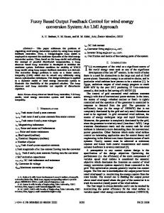
2. Wind Turbine Model The model of the WT is shown in the high level block diagram in Fig. 1. The plant model is composed of a wind model and blade torque calculation, a five mass torsional system, and a detailed model of a synchronous generator connected through a single transmission line to an infinite bus. Dynamics involved in sensing the plant outputs which are shaft speeds ( A u ) , terminal voltage (AVO, and electrical power ( A P , ) are included in the plant. The actuator dynamics representing the blade pitch hydraulic control (0) and the exciter power source supplying the generator field voltage (Vfd),are also included in the plant. The dynamic order of the plant model is 24. The output feedback control appliesstaticand dynamic compensation to the plant measurable system variables to generate control signals. The wind model and calculation of mechanical shaft torqueinvolvenonlinear functional relationships without dynamics. Wind models of gusts or sinusoidal forcing are available, and full rotor immersion assumed. The basic equation that relates wind velocity to available mechanical power is given by:

P = npV3R2C,/2

(9)

where p is the mass density of air, V is the wind velocity, R is the rotordiameter, and C , is a power coefficient representing aerodynamic efficiency of the blades. The power coefficient, C,, is anonlinear function of wind speed and blade pitch angle. InfInite Wlnd and

(7)

Biace

Toraue Co:cs

Synchronous Generator XT

The closed loop is

X = (A + BKC)x = A c L x ,

(8)

andthe matrix AcL has the r desired eigenvalues and eigenvectors. If the remaining n-r eigenvalues of AcL have negative real parts,thiscontrol is the solution to a suboptimal output feedback control problem [8]. Forthederivation of these equations, the cost corresponding to the output feedback design and the relation of this design method to others in the control literature, the readershouldrefer to [8]. This paper focuses on the practical aspects of using this design method in developing output feedback controls for wind turbine generators.

Paper Outline The paper is organizedas follows: Section 2 describes the

WT model. Section 3 presents the control design method and the resulting control. Simulation results, which demonstrate the efficacy of this contzol in the W application, are then described in Section 4. This is followed by conclusions in Section 5. 24

Y =

lbL.BVt.6Pel'

Dynmnlcs

I

Fig. 1. Block diagram of WT model,

The operating regimes of the WT can be illustrated by considering Fig. 2 which shows normalized electrical output power plotted as a function of wind speed. As shown in this figure, the two WT operating regimes are determined by wind speed. Inthe subrated power regime the generator operates below rated power. Here the blade pitch control can be used to provide damping using speed measurements. The shape of the curve in this regime reflects the basic law of power production, in which the power is proportional to the cube of wind velocity, and the power coefficient representing the control

systems magazine

Rated Power

20

10

30

40

Wnd Speed at the Hub (MPH)

Fig. 2.

WT operating regimes.

aerodynamic efficiency. The second regime of WT operation occurs when sufficient wind is available for rated outputpower. In this regime the blade pitch control regulates unit output power to generator rating in addition to providing damping. The nonlinear character of the blade pitch cohtrol path can be seen in Fig. 3 which plots the sensitivity of changes in normalized outputpower to changes in blade pitch angle, as afunction of wind speed in miles per hour. There is almost a three to one change in effective gain change over the plottedoperating region corresponding to rated electrical power from the generator. Considering the subrated power region as well, the gain varies by anorder of magnitude. The implication of this gain change in designing the control isdiscussed in the following section as it relates to the choice of operating point for the control design.

I

WINDSPEED

Fig. 3.

(MPHI

Sensitivity of normalized output power to wind speed.

L

September 1982

The torsional systemmodel is composed of the equivalent lumped inertias, spring constants, and damping factors for A schematic representation of the thefivemasssystem. torsional system is shown in Fig. 4. The five-mass torsional system gives rise to four oscillatory modes, two of which involve the blades, one which represents the generator and gearboxagainst the hub (16.6 d s ) , and the local mode, where the five masses swing together with respect to their common reference frame, (1.45 r / s ) . The blade flap mode where the blades are moving against one another does not couple into the generator; the blade torsional mode, where the blades swing together against the hub and generator, (4 r / s ) couplesintothegenerator response. A goal in the control design is to add damping to the local mode while at thesame time not significantly destabilizing the blade torsional mode.

1 -zw-

Hub

I

I]

Gear Box

9

Gen

Blade 2

U Fig. 4.

Torsionaldynamic model.

The conventional model of the electrical dynamics of the synchronousgenerator uses a direct and quadrature axis representation with a stator circuitand two rotor circuits per axis [ 121. The resulting model is of fourth order after the usual assumption of neglecting the fast dynamics due to stator transients [ 131. The sensorand actuator dynamics are represented by first order time constants, in some cases with nonlinearities due to systemsaturationcharacteristics. Linear dynamics are involved in sensing speed and electricalpower. The actuator thatcontrolsbladepitchangle has a rate limit dueto available hydraulic pressure in the servo-control. The field voltage controlpath has asaturation type nonlinearity due to the magnetic circuits in the rotating exciter. These limits canpotentiallyaffect the transient nonlinear simulation results. Thesimulation program used in the wind turbine analysis, described in Ref. [14], has the capability of both nonlineartime simulation and lineaiized state-space analysis. The state matrices used as a basis for the control design were generated for a number of different operating points by the simulation software. The ability to generate open loop stateLmatrices and check the closed loop control design with the full nonlinearsimulation is key to the design process. 25

3. Control System Design

twocategories,“friendly” and “unfriendly.” The “friendly” test is one whose wind and network conditions change littleduring the run. In the “unfriendly” test, the WT is subjected to severe disturbances, both electrical (faults) and mechanical (low probability, wide variation wind profiles).

As discussed above, there are two control inputs to the wind turbine, the field voltage of the synchronous machine and the pitch angle of the turbine blades relative to the wind. When the wind turbine is operating above rated conditions, there are two important performance goals which must be met, regulation of the terminal voltage of the synchronous Once these stages have been traversed, the design machine and regulation of electrical power. Both of these becomes a candidate for further study. This may involve the conditions are to ensurethat the machine operates within its development of a gain scheduling scheme or of dynamic design range for all disturbances. For safe mechanical stress compensators. These design issues are not described here. levels in the shaft, power oscillations may only infrequently In practice, we found these stages a powerful approach be allowed to exceed 40% above rated power. Steady-state for treating new control problems. The f i s t four stages tend voltage regulation should be such that voltage error is less to run together since for any final design, the control design than 1/2%, and transient voltage swings to less than 2% for process may have started overa number of times. The windgusts. With these performance goals in mind, we following paragraphs summarize some of our experiences in proceedto present the control design method and the developing a control for the wind turbine. resulting design. It wasclearearly in the design process that a high The goal of the control design process is to develop a weighting on terminal voltage error, A V , , was needed to control u = K y such that the above performance spec- provideadequate voltage regulation. In addition, some ifications are met by the closed loop system. The control weights on the integrals, J A V , , and electrical power error, design process followed in this application is broken into S A P , , were needed to allow the introduction of integral five stages. controls which ensure zero steady-state error. The output 1. Study the linearized model at a number of weights resulting from the iterative design process are as operating points. This includes the study of follows: eigenvalues, eigenvectors and modal observability Output Weight which is used to determine the eigenvalues that primarily influence variables to be regulated. AVt 1.35 X 105 Modal controllability is used to isolate eigenvalues V, SA 5 which are not involved in regulation but may be SAP, 20 adversely affected by a control designed for tight This resulted in the optimal eigenvalue placement shown regulation. 2. Solve an optimal LQR problem. Using information in Appendix A. The next stage in the design was to choose which measurements to use, and which eigenvalues to obtained in the linearized model study, the Q and R retain.Thechoice of measurements is restricted at this matrices in the cost J [Eq. (3)] are determined. point.Onlythosefor which sensor hardware has been This is an interative process. 3. Map the optimal solution u = Gx onto an output specified in the WT design may be used. The number of and which measurements areto be chosen is based on the feedback control u = K y . This stage is achieved by eigenvalues chosen to be retained. The high AV, weight has choosing the measurements to beused from the primary effect on five eigenvalues-local mode and three available ones and choosing the eigenvalues and real electrical machine eigenvalues. Two of these machine eigenvectors to be retained from the optimal eigenvalues combine to create acomplex pair. Tight voltage regulator. The output feedback control is checked regulation can be obtained by retaining the remaining real for realism based on experience. For instance, a eigenvalue which is optimally placed at - 14.7 from - 15.1. sufficiently high voltage error (AV,) feedback gain Thus, the measurement, A V t , is used to retain this. Modal is required in orderto obtain desired voltage AmH (change inhub speed) and observability shows that regulation. A P , are good measurements to retain the new local mode 4. Check the control on linearized models at several operatingpoints.The eigenvalue placements re- placement. In addition the J A V , and S A P , are defined as sulting from the use of u = Ky at several operating measurements and are used to retain the integrator points are examined to see if changes in operating eigenvalue placements. Thus five measurements are used. point will causedifficulties. We may have to The choice to retain a real eigenvalue which decreases in return to the beginning of the control design magnitude (from - 15.1 to - 14.7) may seem counter-inmust realize that the philosophy process from this stage if some eigenvalue tuitive;however,one underlying this designprocess is to retain modes which will placements are not adequate. keep the essential aspectsof the full stateoptimal design. In 5 Perform nonlinear simulation tests which include this case, retaining this eigenvalue achieved this. effects of control rate limits, state and control The resulting output feedback gain takes the form constraints, etc. These tests can be classified into 26

control systems

1.5

3.27 0.006 0.9 171 2.94 0.3 -0.391

1

3.531 AVt SA V ,

M e LS M e J This design was obtained at the cutout wind speed (43 mphs), where the sensitivity of the output power to wind speedishighest.Two oscillatory modes are of interest, local mode and the blade torsional mode. As an illustration of stage 4 in the design process, we consider two operating points within the rated WT operating regime. Case 1 corresponds to operating at the lower end of this regime. Case 2 corresponds to cutout speed. Case 1 Case 2 Speed Wind 32.7 mph 43 mph Local Mode 0.22 0.155 Ratio Damping Blade Mode Ratio Damping 0.24 0.033 These two cases show that a design made at one operating point may not be the best design to use at some other point. For this application, it was found necessary to design the control for Case 2 in order toprovide adequate damping of the blade mode. The next sectionpresents some results obtained from nonlinear simulation tests.

4. Nonlinear Simulation Results The results of nonlinear simulation tests of the control designpresented in the last sectionare shown here. As described in Stage 5 of the design process, these tests fit intotwo categories“friendly” and “unfriendly.” Two types of tests are shown, one the is wind disturbance and the otheristheelectrical system disturbance. Many wind disturbances are used for control evaluation. Two of these wind disturbance tests are shown here. Fig. 5 shows the results of the “friendly” test. In this test ratedpoweroperation is tested with an 11 mph versine starting from an initial velocity of 31 mph wind speed, as measuredat the hub.The versine has a period of 12 seconds. From thisfigure,one may note that electrical power oscillations are within the 40% maximum allowed deviation from rated. In addition, terminal voltage is well within its 1/2% requirement. The local mode oscillation can be perceived in electrical power. The higher frequency oscillation seen in mechanical power is due to the blade torsionalmode. From the comparisons shown in the last section it can be expected that at a higher wind speed, the local mode oscillation will be better damped and the blade torsional modes more pronounced. It is interesting to note that this is rather a benign testing of WT operation; an earlier controllerdesign(not described in this paper) showed tighterregulation of voltage and power for this test but showed sustained oscillations of the blade torsional in the next test. The appellation “friendly” is well suited even

T E W I N A L VOLTAGE

t

55-

.98L

c

27.1 0

4

,

,

,

. .

.

I

.

10

20

TIME I N SECONDS

Fig. 5 . Rated power operation 31 MPH wind 11 MPH versine gust T = 12seconds A

though the gust amplitude is quite large. The resultsofthefirst of the “unfriendly” tests are shown in Fig. 6 . This test is designed to illustrate the response to a more severe mechanical disturbance, a low probability wind gust [3], with a significant range of frequencycomponents and large variation in operating points. As seen in Fig. 6 , terminal voltage is within the 2 percent transient limit and returns to well within the 1/2% steady state limit after the passing of the‘ wind disturbance. Electricalpower,shown in Fig. 6 , is regulated with a maximum deviation near 40%. The blade torsional mode is more pronounced in mechanical power. Its lower damping ratio (due to the higherwind speed) is readily perceivable.

T E R M N A L VOLTAGE

-981

-22

i

554

41. W I N D SPEED

27.1

0

,

.

.

,

.

.

10

.

.

1

.

20

TIME I N SECONDS

Fig. 6.

Response WT to a low probability severe wind gust. ~

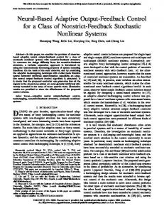
Thefinal, “unfriendly” test is a 5-cycle electrical disturbance (three phase stub fault) with a constant wind input. The result of this test is shown in Fig. 7 . The local mode and blade torsional mode are apparent in mechanical and electricalpower. Terminal voltage decreases to near 0.4 per unit. In response to this, the field voltage regulation

goes to ceiling in an attempt to hold voltage up. Other tests, not shown here, canbe used to examine other tests of subrated aspects of WT operation,forinstance, operation. In this regime, as described earlier, there is no power setpoint. A “washed out” (high pass filtered) power measurement replaces power deviation as an output measurement. New control gains can be computed for this type of operation. Care must be taken to insure that, for winds which vary between subrated and rated WT operation, the changing of control regimes does not result in “hunting. ’’

.

1.5,

.

.

.

.

.

.

.

5. Conclusions The output feedback cone01 design approach, as applied to a M T generator application, is described in this paper. The results of this work suggest that this method can provide a viable approach to the design of controls based on linear quadratic regulator theory when plant nonlinearities andorderpreclude the blind use of a Kalrnan Filter or observer.

.

,MECHANICAL POWER

Appendix A

. .5

20.

ELECTRICAL POWER

.

-

12. 4. -4.

-12. -20.

V

reg

Fig. 7.

~

TIME IN SECONDS

“t

5-cycle three-phase fault X = 0.2 pu from machine terminals

This appendix contains three sets of eignevalues for the linearized model of the WT at 43 mph wind speed. The first setcontains the openloop eigenvalues of the plant, the second set containsthe optimal LQR eigenvalue placement, andthethird set contains the closed loop eigenvalues corresponding to outputfeedack. For the control design given in Section 3, five eigenvalues and eigenvectors of the LQR solution were retained (7, 18, 19, 23 and 24). Other eigenvalues resulting from output feedback differ from the optimal LQR placements. One may note that the remaining 19 eigenvalues change when output feedback replaces full statefeedback.However,the final design provides the desired performance.

EIGENVALUES

OPEN LOOP CLOSED Real Imaginary 1 3 4 5 6 7 8 9 10 11 12 13 14 15 16 17 18 19 20 21 22 23 24

- -393.0 -84.0 -55.6 -38.7 -2.32 -2.32 -15.1 -6.3 -0.213 -10.0 -10.0 - 10.0 -5.0

-0.53 -0.53 -0.33 -0.33 -0.044 -0.044 -0.1 -0.1 -0.1 -0.0 -0.0

0 0 0 0 16.6 -16.6 0 0

0 0 0 0 0

4.22 -4.22 4.12 -4.12 1.46 - 1.46 0 0 0 0 0

FEEDBACK OUTPUT OPTIMAL LOOP Real Imaginary -393.0 -84.0 -55.6 -38.8 -2.2 -2.2 *-14.7 - 10.2 -10.2 - 10.0 -10.0 - 10.0 -5.0

-0.554 -0.554 -0.33 -0.33 *-0.351 *-0.35 1 -0.1 -0.1 -0.1 *-0.334 *-0.017

0 0 0 0 17.0 -1 7.0 0 8.45 -8.45 0 0 0 0

4.23 -4.23 4.12 -4.12 1.53 - 1.53 0 0 0 0 0

-

CLOSED LOOP Imaginary Real

-

0 -393.0 -84.0 -55.6 -39.8 0 15.8 -2.75 -2.75 -15.8 Generator *-14.7 0 -2.59 9.34 -2.59Dynamics -9.34 -10.0 -9.93 -9.84 0 -4.8 1 0 -0.131 3.98 -0.131 -3.98 Blade 2 4.1 -0.33 -0.33 -4.12 *-0.351 1.53 *-0.3 5 1 -1.53 -0.1 -0.1 -0.098 0 *-0.334 0 *-0.017 0

1

}

Frequency Sensor Torsional Dynamics Mode Representing Against Hub Voltage Regulation Sensor Dynamics

1 1 1

BladePitchActuator Blade Torsional Mode Flap Mode Local Mode

1

Filters Integrator Dynamic

* Eigenvalues retained in output feedback‘design. 28

control systems magazine

References W. H. Robbins and R. L. Thomas, “Large Horizontal Axis Wind TurbineDevelopment,” NASA TM-79174 or DOE/NASA 105979/2, Wind Energy Innovative Sys. Conf., Colorado Springs, May, 1979. R. S . Barton and W. C. Lucas, “Conceptual Design of the 6 MW Mod-SA Wind Turbine Generator,” Presented at the Fifth Biennial Wind Energy Conference and Workshop, Washington, DC, Oct. 5-7,1981. “System Dynamics of Multi-Unit Wind Energy Conversion SystemsApplication,” Final Report 78SDS4206, prepared for DOE/ERDA,Feb. 15, 1978. E. N.Hinrichsen, et al., “MOD-2 Wind Turbine Farm Stability Study,” NASA report CR-165156, June, 1980. 0.Wasynczuk, D. T. Man, and J. P. Sullivan, “Dynamic Behavior of aClass of Wind Turbine Generators During Random Wind Fluctuations,” Paper presented at 1981 IEEE PES Winter Meeting, Atlanta, GA. J. Medanic, “On Stabilization and Optimization by Output Feedback,” 12th Annual Asilomar Conference on Circuits and Systems, Pacific Grove, CA, Nov. 1978. J. Medanic, “Design of Low Order Optimal Dynamic Regulators for Linear Time-Invariant Systems,” 1979 Conference on Information Science and Systems. W. E. Hopkins, Jr.,J. Medanic and W. R. Perkins, “Output Feedback Pole Placement inthe Design of Suboptimal Linear Quadratic Regulators,” Inr. J . Control. 1981. B . D. 0.Anderson and J. B . Moore, LinearOptimalControl, Prentice Hall, Inc., Englewood Cliffs, NJ, 1971. 0. A . Solheim, “Design of Optimal Control Systems with Prescribed Eigenvalues,” Int. J . Control, vol. 15, no2 1, pp. 143160,1972. C. A. Harvey and G . Stein, “Quadratic Weights for Asymptotic Regulator Properties,” IEEE Trans. on AutomaticControl, vol. AC-23, pp. 378-387, 1978. W. Janischewskyj and P. Kundur, “Simulation of the Non-Linear Dynamic Response of Interconnected Synchronous Machines,” IEEE Trans. PAS, Sept./Oct. 1972. T. J . Hammons and D. J. Winning, “Comparison of SynchronousMachine Models in the Study of the Transient Behavior of Electrical Power Systems,” Proc. IEEE, vol. 118, No. 10, Oct. 1971. E. V . Larsen and W. W. Price, “MANSTAB/POSSIM Power System Dynamic Analysis Programs-A New Approach Combining Non-linear Simulation and Linearized State-Space/Frequency Domain Capabilities,” IEEEPICAConference, Toronto, May 1977.

S. Harold Javid joined the Electric Utility System Engineering Department of the General Electric Company in 1980 where he is involved

September 1982

in theapplication of modem concepts to electric power systems. He received his B . S . , M.S. and Ph.D. degrees in electrical engineering from the University of Illinois in Urbana, Illinois, in 1973, 1976 and 1978, respectively. From 1977 to 1980, he was employed by Systems Control, Inc., in Palo Alto, California. where he worked on ootimal scheduling and control problems. Dr. Javid is a member of Phi Kappa Phi and the IfEE.

Alexander Murdoch received his B.S.E.E. degree from Worcester Polytechnic Institute in 1970, and the M.S.E.E. and Ph.D. degrees from Purdue University in 1972 and 1975, respectively. He has been with GeneralElectric Company since 1975, working in the Electric Utility System Engineering Department. His recent work has included the design and performance evaluation of control systems under DOE funded work on the development of MOD- 1 and MOD-5 wind turbines for operation in a utility systemenvironment. Other areas of interest include digitally based control forpower system application, non-linear control concepts to enhance transient stability, and development of improved dynamic modeling tools. He is a member of IEEE, Eta Kappa Nu, and Mu Epsilon’ and holds the position of adjunct assistant professor at Union College in Schenectady, New York.

James R. Winkeiman was born on August 2, 1949 in Woodstock, Illinoise. He received his B.S.E.E. with honors in 1972; his M.S. and Ph.D. degrees in electrical engineering in 1973 and 1976, respectively, from the University of Wisconsin, Madison. From 1973 to 1976, he was employed as a research assistant by the Superconducting Energy Storage Project at the University of Wisconsin. Since 1976, he has been with the GeneralElectric Company inthe System Dynamics and Control subsection of the Electric Utility Systems Engineering Department where he has been involved in the study and simulation of power system dynamics. In addition to power systems, his interests include alternate energy sources and modem control theory, He is a member of IEEE, Tau Beta Pi and Phi Kappa Phi.

29