Oct 18, 2017 - Jâ1 q ,. (3) where Jq is the quantum Fisher information ma- trix (QFIM) with ...... [39] P. A. Knott, T. J. Proctor, A. J. Hayes, J. F. Ralph, P. Kok and ...
Control-enhanced multiparameter quantum estimation Jing Liu and Haidong Yuan
arXiv:1710.06741v1 [quant-ph] 18 Oct 2017
Department of Mechanical and Automation Engineering, The Chinese University of Hong Kong, Shatin, Hong Kong Most studies in multiparameter estimation assume the dynamics is fixed and focus on identifying the optimal probe state and the optimal measurements. In practice, however, controls are usually available to alter the dynamics, which provides another degree of freedom. In this paper we employ optimal control methods, particularly the gradient ascent pulse engineering (GRAPE), to design optimal controls for the improvement of the precision limit in multiparameter estimation. We show that the controlled schemes not only capable to provide a higher precision limit, but also have a higher stability to the inaccuracy of the time point performing the measurements. This high time stability will benefit the practical metrology where it is hard to perform the measurement at a very accurate time point due to the response time of the measurement apparatus.
I.
INTRODUCTION
Quantum metrology has seen a rapid development recently [1–21], due to its wide applications in quantum imaging [22, 23], quantum sensing [24] and quantum Hamiltonian identification [25–28]. In most of these applications there are usually multiple unknown parameters, which falls in the subject of multiparameter quantum estimation. Due to its generality, multiparameter quantum estimation is gaining increasing attention. The recent discovery that simultaneous estimation of multiple parameters can provide a higher precision limit than estimating each parameter individually [29–35] further prompts the development of this field [30]. Most existing schemes in multiparameter quantum estimation assume the dynamics is fixed, focus on the identification of the optimal probe states and optimal measurements [29–42]. In practice, however, additional controls usually can be employed to alter the dynamics for further improvement of the precision limit. Systematic methods to obtain optimal controls for the improvement of the precision limit in multiparameter quantum estimation are highly desired. Controls have been recently employed to improve the precision limit for single-parameter quantum estimation [43–45]. For multiparameter quantum estimation, systematic methods to obtain the optimal controls are still lacking, so far optimal controls have only been obtained under unitary dynamics [46]. In this paper we employ the gradient ascent pulse engineering (GRAPE) [47] to obtain optimal controls for multiparameter quantum estimation under general Markovian dynamics, this provides a systematic method on the design of optimally controlled schemes for multiparameter quantum estimation. GRAPE has been widely applied as the pulseengineering technique in quantum information, including the implementation of logic gates for spin systems [48], Bose-Einstein condensates [49] and nitrogen-vacancy centers [50, 51]. GRAPE allows a high flexibility in the designed pulse shapes and no pulse families need to be assumed in advance [47]. However, if practical con-
straints do exist, they can also be easily incorporated into GRAPE [52]. Thus, GRAPE provides a versatile tool for designing controlled schemes for quantum parameter estimation [45]. Controls can not only improve the sensitivity, but also improve the stability, which is another important factor to consider in practical quantum metrology [24, 53]. In practice the measurement apparatus usually has a response time, so the actual time point performing the measurements may be different from the theoretical value. Thus, the stability of the precision limit to the inaccuracy in the measurement time are important and needs to be considered. We provide several examples to show the advantages of the controlled schemes and demonstrate that controls obtained from GRAPE can improve both the precision limit and the stability. Specifically we studied the single- and two-spin systems with dephasing noises and demonstrated the improvement of the sensitivity and the stability provided by the controls. II.
MULTIPARAMETER ESTIMATION
Typically to estimate multiple parameters encoded in some quantum state ρ~x , where ~x = (x1 , x2 , ..., xd ), one needs to perform a set of positive-operator valued P measurements (POVM) {E(y)} ( y E(y) = 11 with 11 the identity) on the state, which will give the result y with probability py|~x = Tr(ρ~x E(y)). From the measurement result one can then construct an estimator ~x ˆ = (ˆ x1 , x ˆ2 , ..., x ˆd ). According to the Cramér-Rao bound, the covariance of any unbiased estimator is bounded below by the (classical) Fisher information matrix as [54, 55] C ≥ Fcl−1 .
(1)
Here C denotes the covariance matrix with the entries P Cαβ := y (ˆ xα − xα )(ˆ xβ − xβ )py|~x , α, β ∈ {1, 2, ..., d}, and Fcl denotes the classical Fisher information matrix (CFIM) with the αβth entry given by Fcl,αβ :=
X (∂xα py|~x )(∂xβ py|~x ) y
py|~x
.
(2)
2 The covariance matrix can be further bounded by the quantum Fisher information matrix C ≥ Fcl−1 ≥ Fq−1 ,
(3)
where Fq is the quantum Fisher information matrix (QFIM) with the αβth entry given by Fq,αβ = 1 2 Tr(ρ{Lα , Lβ }). Lα is the symmetric logarithmic derivative for xα which is the solution to the equation ∂xα ρ = (ρLα + Lα ρ)/2. In multiparameter quantum estimation the bound given by the QFIM is usually not saturable [30, 56–58], therefore we will focus on the classical Cramér-Rao bound. In this paper we will take Pd 2 |δ~x ˆ|2 := ˆi as the figure of merit, from the i=1 δ x Cramér-Rao bound we have |δ~x ˆ|2 ≥ TrFcl−1 .
(6)
as an objective function to be maximized. However, the obtained controls will be eventually evaluated by their effects on the figure of merit TrFcl−1 , which characterizes ˆ. In many cases this provides the precision limit of δ~x efficient algorithms lead to near optimal controls. III.
ALGORITHM
(7)
where L(ρ) = −i[H, ρ] + Γ(ρ), here Γ(ρ) describes the effect of the noises and H denotes the Hamiltonian. The Hamiltonian can be decomposed as [47, 59] H = H0 (~x) +
p X
k=1
Vk (t)Hk ,
Vk (j) ! Vk (j) + ✏ · gradient Calculate the objective function f0 (T )(Fcl,e (T )) Calculate the gradient f0 (T ) Vk (j)
✓
Fcl,e (T ) Vk (j)
◆
Convergence
STOP
Figure 1. (Color online) The flow chart of GRAPE algorithm for multiparameter estimation.
where H0 (~x) is the Hamiltonian for the free evolution which contains the unknown parameters ~x, Pp V (t)Hk is the control Hamiltonian with Vk (t) dek k=1 notes the amplitude of kth control field. The solution of Eq. (7) at the target time T can be approximated as ρ(T ) = Πm i=1 exp(∆tLi )ρ(0), with Li the super-operator for the ith time step and m = T /∆t sufficiently large, here the multiplication in ρ(T ) is taken from right to left in the increasing order of i. We then employ gradient ascent pulse engineering (GRAPE) [47] to obtain optimal controls that can maximize f0 (T ) (Fcl,e for two-parameter estimation). The flow of the algorithm, shown in Fig. 1, is as following: 1. guess a set of initial values for Vk (j) (Vk (j) is the kth control at the jth time step); 2. evolve the dynamics with the controls; 3. calculate the objective function f0 (T ) (Fcl,e for twoparameter estimation); � δFcl,e 0 (T ) 4. calculate the gradient δf δVk (j) δVk (j) for two� parameter estimation ; 0 (T ) 5. update Vk (j) to Vk (j) + � δf δVk (j) ;
We consider the systems whose dynamics can be described by the master equation ∂t ρ(t) = L[ρ(t)],
Evolve the dynamics with the controls
(4)
Thus the controls should be designed to minimize TrFcl−1 . For the case with only two parameters, Eq. (4) reduces −1 to |δ~x ˆ|2 ≥ Fcl,e [32], where Fcl,e = det Fcl /TrFcl , here det(·) denotes the determinant. For the cases with more than two parameters, it is in general difficult to obtain the analytical expression for Fcl−1 directly, which means this function is not very friendly to a gradient-based algorithm in general as in each iteration the gradient needs to be evaluated numerically which is very demanding computationally. Usually the bound will be further relaxed to ease the computation. Since [Fcl−1 ]αα ≥ 1/Fcl,αα , we then have X 1 . (5) TrFcl−1 ≥ Fcl,αα α We will then also take the following quantity !−1 X 1 f0 (T ) = Fcl,αα (T ) α
Guess a set of initial values of Vk (j)
(8)
6. go to step 2 until the objective function converges. The detailed calculation of the gradient for f0 (T ), which is based on the gradient of the entries of CFIM and an essential step for GRAPE, can be found in appendix A. GRAPE can be further improved via the quasiNewton optimization [60], which utilize the gradient history to construct an approximation to the Hessian matrix. Davidon-Fletcher-Powell formula [61] and BroydenFletcher-Goldfarb-Shanno algorithm [62] are two well applied methods for this construction. This quasi-Newton
3 optimization can also be utilized here in quantum parameter estimation for the improvement of GRAPE performance. Apart from GRAPE, other optimization methods, such as Krotov’s method [63–67], hybrid update method [64] and hybrid optimization method [66] can all be employed for controlled quantum parameter estimation. The comparison of these methods for quantum parameter estimation will be studied in future works.
IV.
(a) Example 1
APPLICATION
We demonstrate the effect of controls with several examples in Hamiltonian parameter estimation.
A.
Noiseless scenario
Example 1 : Consider a two-qubit system where one qubit is in a magnetic field and the other qubit acts as an ancillary qubit. The Hamiltonian of this system is H = H0 + Hc (t) where ~ · ~σ (1) , H0 = B (1)
(1)
(1)
(9)
(b) Example 2
(1)
~σ (1) = (σ1 , σ2 , σ3 ) with σi = σi ⊗ 112 , here σ1 , σ2 , σ3 are Pauli matrices, 112 denotes the 2 by 2 identity matrix. (2) (2) (2) Similarly we will use ~σ (2) = (σ1 , σ2 , σ3 ) to denote (2) σi = 112 ⊗ σi . With the absence of control, the QFIM can be attained via Bell measurement [46]. For controlled scheme, the local controls on the qubits X ~i (t) · ~σ (i) V (10) Hc (t) = i=1,2
are employed. This problem has been studied previously and analytical solutions for optimal controls have been obtained [46]. It has been shown that the optimal controls is to reverse the free evolution and the optimal initial state is any maximally entangled state, such as √12 (|00i ± |11i), and the optimal measurement is the projective measurement on the Bell basis: |Φ± i = √12 (|00i ± |11i) and |Ψ± i = √1 (|01i ± |10i). The precision limit for the three pa2 ~ = rameters (B, θ, φ) characterizing the magnetic field B (B sin θ cos φ, B sin θ sin φ, B cos θ) under optimal control is [46] TrFcl−1 =
3 . 4T 2
(11)
As a confirmation of validity of GRAPE, we compare the performance of the controls obtained from GRAPE (the objective function is f0 ). It can be seen from Fig. 2(a) that the performance of the controls (red dots) obtained from GRAPE coincides with the analytical solutions,
(c) Example 3
Figure 2. (Color online) TrFcl−1 as a function of target time T . The solid black and dashed blue line represent the noiseless and noisy performance of non-controlled schemes for (a) example 1; (b) example 2 and (c) example 3.The red dots and cyan stars represent noiseless and noisy performance of controlled schemes in three examples. The controls are obtained via GRAPE with the objective function f0 (T ) for (a) and (b) and Fcl,e for (c). The dotted green line represent the optimal total precision limits. The dephasing rate in (a) is γ = 0.2 and in (b) and (c) is γ1 = γ2 = 0.1. The true values in (a) are 1, π/4, π/4 for B, θ, φ; in (b) are 1, 1.2, 0.1 for ω1 , ω2 , g; in (c) are 1, 1.2 for x1 , x2 .
4 which shows that GRAPE is capable to identify the optimal controls in this case. Example 2 : Next we consider the Hamiltonian estimation for a two-qubit system with ZZ coupling, which is a widely used model under strong field. The Hamiltonian in this case is (1)
(2)
(1) (2)
H0 = ω1 σ3 + ω2 σ3 + gσ3 σ3 ,
scheme is Fcl = 4T 2 112 , this indicates that the local measurement, E± , is only optimal for x2 . But if we add controls that obtained from GRAPE with Fcl,e as the objective function, then the precision limit(red dots in Fig. 2(c)) can reach the optimal values even under the local measurement E± .
(12) B.
where ω1 , ω2 and g are the parameters to be estimated. We first consider the case without controls. The optimal probe state for this system is | + +i where |+i = √1 (|0i + |1i) (see detailed derivations in appendix C) 2 and the corresponding QFIM is Fq (T ) = 4T 2 113 (113 denotes the 3 by 3 identity matrix). This QFIM is at(1) (2) tainable, which is due to the fact that σ3 , σ3 and (1) (2) σ3 σ3 commute with each other. The optimal measurement exists [29, 30] but practically challenging to implement. In practice, usually the local measurement E± = {| + +ih+ + |, | + −ih+ − |, | − +ih− + |, | − −ih− − |} is used instead, under this local measurement, the precision (solid black line in Fig. 2(b)) is typically much worse than the optimal measurement, and it oscillates with time, which indicates that the time stability of the local measurement is quite poor, i.e., a small error in the time point chosen to perform the measurement can result very different precisions. Now if controls are employed, both the precision and the time stability can be improved. This can be seen from Fig. 2(b), the precision of controlled scheme under the local measurement E± (red dots in Fig. 2(b)) essentially coincides with the precision under the optimal measurement (dotted green line in Fig. 2(b)), it also does not oscillate as in the non-controlled case. This shows that controls can improve both the precision limit and the time stability. Example 3 : In this example we consider the Hamiltonian estimation with XXZ coupling. The Hamiltonian is � � (1) (2) (1) (2) (1) (2) H0 = −x1 σ1 σ1 + σ2 σ2 − x2 σ3 σ3 , (13) where x1 and x2 are coupling parameters to be estimated. First without controls, the optimal QFIM is � � 8T 2 0 Fq,opt = , (14) 0 4T 2
which can be attained with the optimal probe state |ψ0,opt i = √12 |0i(|0i + i|1i) (see details in appendix D). The optimal total precision limit for the non-controlled scheme then reads −1 TrFq,opt =
3 . 8T 2
(15)
In this case the QFIM is attainable as the generators for x1 and x2 commute. However, if we use the more practical local measurement E± , the CFIM for non-controlled
Noisy scenario
We now consider the dynamics with dephasing noises in all examples discussed above. Example 1 : Again we consider a two-qubit system where the magnetic field only acts on the first qubit and the second qubit acts as an ancillary system. For example, in Nitrogen vacancy center, the electron spin can act as the sensing qubit while a neighboring nuclear spin can act as an ancillary system. Recall that the Hamiltonian ~ · ~σ (1) and is given by H = H0 + Hc (t) where H0 = B P (i) ~i (t) · ~σ . Hc (t) = i=1,2 V Assume that the sensing qubit (first qubit) suffers from the dephasing noise, the dynamics is then described by the master equation � γ � (1) (1) ∂t ρ = −i[H, ρ] + σ3 ρσ3 − ρ . (16) 2 Figure 2(a) (cyan stars) shows the advantages of controlled scheme in improving the precision limit. From the figure it can also be seen that the controls also suppress the oscillations, thus improve the time stability. Example 2 : Consider the Hamiltonian with ZZ cou(1) (2) pling H = H0 + Hc (t) where H0 = ω1 σ3 + ω2 σ3 + P (1) (2) ~i (t) · ~σ (i) . With the presgσ3 σ3 and Hc (t) = i=1,2 V ence of dephasing, the dynamics is described by � X γi � (i) (i) σ3 ρσ3 − ρ , (17) ∂t ρ = −i[H, ρ] + 2 i=1,2 where γi is the dephasing rate for ith qubit. Fig. 2(b) shows that the controlled scheme improves the precision limit under the local measurement E± . It can also be seen that the controls suppressed the oscillations in the precision limit, thus improved the time stability. Example 3 : Consider the Hamiltonian estimation with (1) (2) (1) (2) XXZ coupling where H0 = −x1 (σ1 σ1 + σ2 σ2 ) − (1) (2) x2 σ3 σ3 and the control Hamiltonian is Hc (t) = P ~ σ (i) , both qubits have the dephasing. The i=1,2 Vi (t) · ~ master equation for this system is in the form of Eq. (17), and we will assume the dephasing rates are the same for both qubits, i.e., γ1 = γ2 = γ. The CFIM for noncontrolled scheme under the practical local measurement E± is given by (see detailed derivation in appendix D) � � δ+ + δ− δ+ − δ− Fcl = 2T 2 , (18) δ+ − δ− δ+ + δ− where δ± :=
cos2 [2T (x1 ± x2 )] . e2γT − sin2 [2T (x1 ± x2 )]
(19)
5 The precision limit for non-controlled scheme is then � � 1 1 1 −1 TrFcl = + . (20) 4T 2 δ+ δ− It can be seen that when 2T (x1 ± x2 ) = π/2 + nπ (n = 0, 1, 2...) this precision blows up, which corresponds to the peaks in Fig. 2(c). After adding controls, which are obtained from GRAPE with the objective function Fcl,e , the precision limit (cyan stars in Fig. 2(c)) is improved compared the uncontrolled case (dashed blue line in Fig. 2(c)). Also, the oscillations is suppressed, indicating that the controlled scheme provides a higher time stability.
(1)
m = iDj+1 Hk× ρj . One then can obtain � � �� δ ∂xα py|~x m = −i∆tTr E(y)∂xα Dj+1 Hk× ρj δVk (j) n h � × m = −i∆tTr E(y) ∂xα Dj+1 Hk ρj io m +Dj+1 Hk× ∂x ρj . (A3)
where Mj
Based on Ref. [45], we know m ∂xα Dj+1 = ∆t
m X
i=j+1
∂xα ρj = ∆t
j X i=1
V.
SUMMARY
In this paper, we employed the optimal control method, GRAPE in particular, in designing optimal controls for the improvement of the precision limit in multiparameter quantum estimation. Advantages on the precision limit of controlled schemes are demonstrated through three examples, including the estimation of a magnetic field, Hamiltonian estimation with ZZ and XXZ couplings. The controls not only improve the precision limit, but also the time stability, especially for noisy systems.
ACKNOWLEDGMENTS
Appendix A: Calculation of gradient for the entries of CFIM
+
j X
py|~x
j m Dj+1 Hk× Di+1 H˙ 0× ρi
i=1
�i .
(A6)
for j = m, there is � � � δ ∂xα py|~x = −i∆tTr E(y)Hk× ∂x ρm δVk (m) # " m X j × × 2 Di+1 H˙ 0 ρi . = −∆ tTr E(y)Hk Thus, combined above equations, we have � n h io δ ∂xα py|~x (2) (3) = −∆2 tTr E(y) Mj,α + Mj,α , δVk (j) (2)
(3)
where Mj,α and Mj,α are Mj,α = (3) Mj,α
j X i=1
j m Dj+1 Hk× Di+1 H˙ 0× (ρi ),
= (1 − δjm )
.
(A1)
where py|~x = Tr(ρ(T )E(y)). P Here E(y) is a POVM measurement which satisfies y E(y) = 11. To calculate the gradient, we first need to know � � δpy|~x δρ(T ) = Tr E(y) δVk (j) δVk (j) � � δρj m = Tr Dj+1 E(y) δVk (j) h i (1) = −∆tTr E(y)Mj , (A2)
m X
(A7)
m ˙× i Di+1 H0 Dj+1 Hk× (ρj ).
i=j+1
It is known that the entry of CFIM is
y
(A5)
where H˙ 0× = [∂xα H0 , ·]. For j 6= m, � m h� X δ ∂xα py|~x m ˙× i = −∆2 tTr E(y) Di+1 H0 Dj+1 Hk× ρj δVk (j) i=j+1
(2)
Fcl,αβ =
j Di+1 (∂xα Li ) ρi ,
(A4)
i=1
H.Y. acknowledges partial financial support from RGC of Hong Kong with Grant No. 538213. J.L. acknowledges partial financial support from the Natural Science Foundation of Zhejiang Province under Grant No. LY18A050003. We would like to thank the anonymous referees for the helpful suggestions.
X (∂xα py|~x )(∂xβ py|~x )
m i Di+1 (∂xα Li ) Dj+1 ,
Utilizing above expressions, the gradient for Fcl,αβ is � � δFcl,αβ (T ) ˜ 2,αβ M(1) = ∆tTr L j δVk (j) �i h � ˜ 1,β M(2) +M(3) −∆2 tTr L j,α j,α h � �i (2) 2 ˜ 1,α M +M(3) , (A8) −∆ tTr L j,β j,β ˜ 1,α(β) and L ˜ 2,αβ are where L X � ˜ 1,α(β) = ∂xα(β) ln py|~x E(y), L y
˜ 2,αβ = L
X y
∂xα ln py|~x
�
(A9)
� ∂xβ ln py|~x E(y). (A10)
6 For two parameter estimation, the objective function is Fcl,e =
2 Fcl,αα Fcl,ββ − Fcl,αβ det Fcl = . TrFcl Fcl,αα + Fcl,ββ
(A11)
The corresponding gradient is 2 2 + Fcl,αβ δFcl,e X Fcl,ββ δFcl,αα 2Fcl,αβ δFcl,αβ = − 2 δVk (j) δVk (j) TrFcl δVk (j) Tr Fcl α6=β
(A12) For parameter estimation with more than two parameters, recall the objective function is f0 (T ) =
X
1
!−1
.
(A13)
δf0 (T ) X f02 (T ) δFcl,αα = . 2 δVk (j) Fcl,αα δVk (j) α
(A14)
α
Fcl,αα (T )
The gradient of f0 (T ) then reads
Appendix B: Calculation of noisy CFIM and QFIM in the estimation of magnetic field
In this appendix we show the detailed calculation in the estimation of magnetic field. Recall that the scenario is a two-qubit system where the magnetic field only acts on the first qubit and the second qubit acts as an ancillary system, the Hamiltonian is given by H = H0 + Hc (t) where ~ · ~σ (1) , H0 = B (1)
(1)
(1)
(B1)
Fcl,θθ Fcl,BB
Fcl,Bθ
For the further calculation, we rewrite the corresponding � density� matrix in block form |ψ(T )ihψ(T )| = X Y 1 , where X, Y and Q are 2 by 2 matrices. 2 Y† Q Recall the master equation involving the noise is � γ � (1) (1) σ3 ρσ3 − ρ . (B3) ∂t ρ = −i[H, ρ] + 2 The solution for above equation can be expressed in the following form � � 1 X e−γT Y ρ(T ) = . (B4) Q 2 e−γT Y † Performing the Bell measurements, the probability distribution is 1 [(1 + e−γT )cos2 (BT )+(1 − e−γT )sin2 (BT )cos2 θ], 2 1 = [(1 − e−γT )cos2 (BT )+(1 + e−γT )sin2 (BT )cos2 θ], 2 1 = sin2 (BT ) sin2 θ[1 + e−γT cos(2φ)], 2 1 = sin2 (BT ) sin2 θ[1 − e−γT cos(2φ)]. 2
pΦ+ = pΦ− pΨ+ pΨ−
According to the probabilities, the entries of CFIM can then be calculated as below
(1)
~σ (1) = (σ1 , σ2 , σ3 ) with σi = σi ⊗ 112 , where σ1 , σ2 , σ3 are Pauli matrices, 112 denotes the 2 by 2 iden(2) (2) (2) tity matrix. Similarly we denote ~σ (2) = (σ1 , σ2 , σ3 ) (2) with σi = 112 ⊗ σi . �
With the initial state √12 (|00i+|11i), the evolved state without noise can be straightforwardly obtained in the basis {|00i, |01i, |10i, |11i} as below cos(BT ) − i sin(BT ) cos θ 1 −i sin(BT ) sin θe−iφ . (B2) |ψ(T )i = √ −i sin(BT ) sin θeiφ 2 cos(BT ) + i sin(BT ) cos θ
Fcl,φφ =
4e−2γT sin2 (BT ) sin2 θ sin2 (2φ) , 1 − e−2γT cos2 (2φ)
Fcl,θφ = Fcl,Bφ = 0 and
sin2 (BT ) sin2 θ cos2 θ[(1 + 3e−2γT ) cos2 (BT ) + (1 − e−2γT ) sin2 (BT ) cos2 θ] = 4 sin (BT ) cos θ + [cos2 (BT ) + sin2 (BT ) cos2 θ]2 − e−2γT [cos2 (BT ) − sin2 (BT ) cos2 θ]2 n = 4T 2 cos2 (BT ) sin2 θ + sin2 (BT ) × 2
2
(B5)
�
,
[sin4 θ + e−2γT (1 + cos2 θ)2 ][1 − sin2 (BT ) sin2 θ] + 2e−2γT sin2 θ(1 + cos2 θ)[− cos2 (BT ) + sin2 (BT ) cos2 θ] o , [cos2 (BT ) + sin2 (BT ) cos2 θ]2 − e−2γT [cos2 (BT ) − sin2 (BT ) cos2 θ]2 n = T sin(2BT ) sin(2θ) 1 + sin2 (BT ) × (1 + e−2γT ) cos2 (BT ) sin2 θ + (1 − e−2γT ) sin2 (BT ) cos2 θ sin2 θ − 2e−2γT cos2 (BT )(1 + cos2 θ) o . [cos2 (BT ) + sin2 (BT ) cos2 θ]2 − e−2γT [cos2 (BT ) − sin2 (BT ) cos2 θ]2
Although the CFIM has analytical solution, it is still diffi-
cult to obtain the general solution of TrFcl−1 analytically.
7 Here we consider the case that θ is small. The expression of TrFcl−1 approximates to TrFcl−1 ≈
1 + cos(2BT ) e2γT − cos2 (2φ) θ−2 − 2 1 − cos(4BT ) 2[1 − cos(2BT )] sin (2φ) 1 − 2e2γT + cos(4BT ) − . (B6) 4T 2 [1 − cos(4BT )]
The non-zero eigenvalues of the noisy density matrix are λ± = 12 (1 ± e−γT ), which are independent of the magnetic field. The eigenstates for λ± are |λ+ i = |ψ(T )i and cos(BT ) − i sin(BT ) cos θ 1 −i sin(BT ) sin θe−iφ . (B7) |λ− i = √ i sin(BT ) sin θeiφ 2 cos(BT ) + i sin(BT ) cos θ
It is known that the QFIM can be calculated via the density matrix’s non-zero eigenvalues and corresponding eigenstates [68, 69]. Utilizing above eigenstates, The entries of QFIM can be calculated as below � Fq,BB = 4T 2 cos2 θe−2γT + sin2 θ , (B8)
where ω1 , ω2 and g are the parameters to be estimated. It is known that for pure states, the element of QFIM is Fq,αβ = 4Re h∂α ψ(T )|∂β ψ(T )i
� −h∂α ψ(T )|ψ(T )ihψ(T )|∂β ψ(T )i .
In this case, the evolved state |ψ(T )i = e−iHT |ψ0 i. Utilizing this form, one can have the diagonal entries of the QFIM as below, � � (1) (C3) Fq,ω1 ω2 = 4T 2 1 − hψ0 |σ3 |ψ0 i2 , � � (2) (C4) Fq,ω2 ω2 = 4T 2 1 − hψ0 |σ3 |ψ0 i2 , � � (1) (2) (C5) Fq,gg = 4T 2 1 − hψ0 |σ3 σ3 |ψ0 i2 .
The off-diagonal entries are � � (1) (2) (1) (2) Fq,ω1 ω2 = 4T 2 hψ0 |σ3 σ3 |ψ0 i − hψ0 |σ3 |ψ0 ihψ0 |σ3 |ψ0 i , � � (2) (1) (1) (2) Fq,ω1 g = 4T 2 hψ0 |σ3 |ψ0 i − hψ0 |σ3 |ψ0 ihψ0 |σ3 σ3 |ψ0 i , � � (1) (2) (1) (2) Fq,ω2 g = 4T 2 hψ0 |σ3 |ψ0 i − hψ0 |σ3 |ψ0 ihψ0 |σ3 σ3 |ψ0 i . From the expressions of QFIM, one can see that the optimal QFIM is in the form
and
Fq,θθ
and
n = 4 sin2 (BT ) cos2 θ � �o + sin2 θ e−2γT cos2 (BT ) + sin2 (BT ) ,(B9)
� � Fq,φφ = 4 sin2 θ sin2 (BT ) 1−(1 − e−2γT ) sin2 θ sin2 (BT ) . (B10) The off-diagonal entries are Fq,Bθ = (1 − e
−2γT
)T sin(2BT ) sin(2θ),
(B11)
Fq,max = 4T 2 113 ,
and Fq,θφ = 2(1 − e−2γT ) sin3 θ sin(2BT ) sin2 (BT ). (B13) it can be seen that the Bell measurement fails to be optimal when noise exists.
Appendix C: Detailed calculation in Hamiltonian estimation with ZZ coupling
In this appendix we show the detailed calculation in the hamiltonian estimation with ZZ coupling. The corresponding Hamiltonian is in the form (1)
(2)
(1) (2)
H0 = ω1 σ3 + ω2 σ3 + gσ3 σ3 ,
(C1)
(C6)
where 113 is a 3 by 3 identity matrix. This optimal QFIM can be obtained if the probe state satisfies the following equations (1)
hψ0 |σ3 |ψ0 i = 0,
(C7)
= 0,
(C8)
= 0.
(C9)
(2) hψ0 |σ3 |ψ0 i (1) (2) hψ0 |σ3 σ3 |ψ0 i
Denote the probe state as |ψ0 i = a|00i + b|01i + c|10i + d|11i, above equations are equivalent to |a|2 + |b|2 − |c|2 − |d|2 = 0, |a|2 + |c|2 − |b|2 − |d|2 = 0, |a|2 + |d|2 − |b|2 − |d|2 = 0.
and Fq,Bφ = −2(1 − e−2γT )T sin(2θ) sin θ sin2 (BT ), (B12)
(C2)
(C10) (C11) (C12)
Taking into account the normalization |a|2 + |b|2 + |c|2 + |d|2 = 1, the only solution is |a|2 = |b|2 = |c|2 = |d|2 = 1/4. Thus, the optimal probe state is in the form |ψ0,opt i =
� 1 |00i + eiφ1 |01i + eiφ2 |10i + eiφ3 |11i , 2
where φ1 , φ2 and φ3 are relative phases. The simplest one is φ1 = φ2 =√φ3 = 0, i.e., |ψ0,opt i = | + +i, where |+i = (|0i + |1i)/ 2. Now we discuss the noisy case. Consider the dephasing noise for both qubits, the master equation for the system is � X γi � (i) (i) ∂t ρ = −i[H, ρ] + σ3 ρσ3 − ρ . (C13) 2 i=1,2 The specific solution of ρ(T ) is
8
ρ00 (0) ρ10 (0)ei2(g+ω2 )T −γ2 T ρ20 (0)ei2(g+ω1 )T −γ1 T ρ30 (0)ei2(ω1 +ω2 )T −(γ1 +γ2 )T
ρ01 (0)e−i2(g+ω2 )T −γ2 T ρ02 (0)e−i2(g+ω1 )T −γ1 T ρ03 (0)e−i2(ω1 +ω2 )T −(γ1 +γ2 )T ρ11 (0) ρ12 (0)e−i2(ω1 −ω2 )T −(γ1 +γ2 )T ρ13 (0)ei2(g−ω1 )T −γ1 T , i2(ω1 −ω2 )T −(γ1 +γ2 )T i2(g−ω2 )T −γ2 T ρ21 (0)e ρ22 (0) ρ23 (0)e −i2(g−ω1 )T −γ1 T −i2(g−ω2 )T −γ2 T ρ31 (0)e ρ32 (0)e ρ33 (0)
where ρij (0) is the initial values of the entries for density matrix. For the probe state | + +i, ρij (0) = 1/4 for any i
and j. The probability distribution for the measurement {| + +ih+ + |, | + −ih+ − |, | − +ih− + |, | − −ih− − |} are
o 1n 1 + e−γ1 T cos(2gT ) cos(2ω1 T ) + e−γ2 T cos(2gT ) cos(2ω2 T ) + e−(γ1 +γ2 )T cos(2ω1 T ) cos(2ω2 T ) ,(C14) 4 o 1n p+− (T ) = 1 + e−γ1 T cos(2gT ) cos(2ω1 T ) − e−γ2 T cos(2gT ) cos(2ω2 T ) − e−(γ1 +γ2 )T cos(2ω1 T ) cos(2ω2 T ) ,(C15) 4 o 1n p−+ (T ) = 1 − e−γ1 T cos(2gT ) cos(2ω1 T ) + e−γ2 T cos(2gT ) cos(2ω2 T ) − e−(γ1 +γ2 )T cos(2ω1 T ) cos(2ω2 T ) ,(C16) 4 o 1n p−− (T ) = 1 − e−γ1 T cos(2gT ) cos(2ω1 T ) − e−γ2 T cos(2gT ) cos(2ω2 T ) + e−(γ1 +γ2 )T cos(2ω1 T ) cos(2ω2 T ) .(C17) 4 p++ (T ) =
Appendix D: Detailed calculation in Hamiltonian estimation with XXZ coupling
In this appendix we show the detailed calculation in the Hamiltonian estimation with XXZ coupling. Recall the Hamiltonian for the XXZ model is � � (1) (2) (1) (2) (1) (2) H0 = −x1 σ1 σ1 + σ2 σ2 − x2 σ3 σ3 . (D1) (1) (2)
(1) (2)
(1) (2)
� � (1) (2) and Fq,x2 x2 = 4T 2 1 − hψ0 |σ3 σ3 |ψ0 i2 . diagonal entry is
The off-
(D3)
From these expressions, one can find the optimal QFIM is (in the basis {x1 , x2 }) � � 2T 2 0 Fq,opt = 4 , (D4) 0 T2 which can be obtained when the probe state |ψ0 i satisfies (1) (2)
hψ0 |σ3 σ3 |ψ0 i = 0, +
(1) (2) σ2 σ2 |ψ0 i
(D7) (D8)
Taking into account the normalization relation, above equations can be reorganized into 1 , 2 1 |b|2 + |c|2 = , 2 cos (φc − φb ) = 0, |a|2 + |d|2 =
(D9) (D10) (D11)
where φb and φc are the arguments of b and c, respectively. Any probe state satisfies these conditions is the optimal probe state. One of them is
(1) (2)
Fq,x1 x2 = −4T 2 hψ0 |σ1 σ1 + σ2 σ2 |ψ0 i � � (1) (2) × 1 + hψ0 |σ3 σ3 |ψ0 i .
(1) (2) hψ0 |σ1 σ1
|a|2 − |b|2 − |c|2 + |d|2 = 0, b∗ c + bc∗ = 0.
(1) (2)
Because [σ3 σ3 , σ1 σ1 ] = [σ3 σ3 , σ2 σ2 ] = 0, the diagonal entries for QFIM can then be calculated as � (1) (2) Fq,x1 x1 = 4T 2 2 − 2hψ0 |σ3 σ3 |ψ0 i � (1) (2) (1) (2) −hψ0 |σ1 σ1 + σ2 σ2 |ψ0 i2 , (D2)
(1) (2)
Expand the probe state in the computational basis {|00i, |01i, |10i, |11i}, i.e., |ψ0 i = a|00i + b|01i + c|10i + d|11i, above equations reduce to
= 0.
(D5) (D6)
1 |ψ0,opt i = √ |0i (|0i + i|1i) , 2
(D12)
which will be used as the probe state in the following calculation. The evolved state can then be further calculated as � 1 � |ψT,opt i = √ 2 cos(x2 T ) − e−ix2 T |00i 2 i + √ e−ix2 T cos (2x1 T ) |01i 2 1 − √ sin (2x1 T ) e−ix2 T |10i. (D13) 2
9 Neglecting the global phase e−ix2 T , this evolved state is equivalent to � 1 � |ψT,opt i = √ ei2x2 T |00i +icos(2x1 T )|01i−sin(2x1 T )|10i . 2 (D14) Now we perform a practical measurement {| + +ih+ + |, | + −ih+ − |, | − +ih− + |, | − −ih− − |} and calculate the corresponding CFIM. The probabilities are 1 {1 − sin [2(x1 − x2 )T ]} , 4 1 = {1 − sin [2(x1 + x2 )T ]} , 4 1 = {1 + sin [2(x1 + x2 )T ]} , 4 1 = {1 + sin [2(x1 − x2 )T ]} . 4
p++ =
(D15)
p+−
(D16)
p−+ p−−
(D17) (D18)
The corresponding CFIM is (in the basis {x1 , x2 }) � � 4T 2 0 Fcl = . (D19) 0 4T 2 For x2 , this measurement is optimal, but for x1 , it is not. Thus, it is not optimal for joint measurement. Now we involve the dephasing noise in both qubits. The master equation for the system is � X γi � (i) (i) ∂t ρ = −i[H, ρ] + σ3 ρσ3 − ρ . (D20) 2 i=1,2
The solutions are i ρ01 (T ) = − e(i2x2 −γ2 )T cos (2x1 T ) , 2 1 ρ02 (T ) = − e(i2x2 −γ1 )T sin (2x1 T ) . 2
1 , 2 ρ33 (T ) = ρ33 (0) = 0, −(γ1 +γ2 )T
ρ03 (T ) = ρ03 (0)e
∂t ρ13 = −i2x2 ρ13 − γ1 ρ13 + i2x2 ρ23 , ∂t ρ23 = i2x1 ρ13 − i2x2 ρ23 − γ2 ρ23 .
∂t ρ12 = − (γ1 + γ2 ) ρ12 − i2x1 (ρ11 − ρ22 ) , (D30) ∂t ρ11 = −i2x1 (ρ12 − ρ21 ) , (D31) ∂t ρ22 = i2x1 (ρ12 − ρ21 ) . (D32) Taking into account the initial condition the solution for these differential equations are i ρ12 (T ) = − sin (4x1 T ) e−(γ1 +γ2 )T , 4
p−−
1 1 − e−(γ1 +γ2 )T cos (4x1 T ) − 4x21 2 2 16x21 + (γ1 + γ2 ) +x1
e−(γ1 +γ2 )T (γ1 + γ2 ) sin (4x1 T ) ,(D34) 2 16x21 + (γ1 + γ2 )
and ρ22 (T ) = 1/2 − ρ11 (T ). (D24) (D25)
Next we perform the measurement {| + +ih+ + |, | + −ih+ − |, | − +ih− + |, | − −ih− − |}. The corresponding probabilities are
1� 1 − sin (2x1 T ) cos (2x2 T ) e−γ1 T 4 1� = 1 − sin (2x1 T ) cos (2x2 T ) e−γ1 T 4 1� = 1 + sin (2x1 T ) cos (2x2 T ) e−γ1 T 4 1� 1 + sin (2x1 T ) cos (2x2 T ) e−γ1 T = 4
p++ =
p−+
ρ11 (T ) =
(D23)
For ρ01 and ρ02 , the differential equations are
p+−
(D33)
and
(D22)
∂t ρ01 = (i2x2 − γ2 ) ρ01 − i2x1 ρ02 , ∂t ρ02 = (i2x2 − γ1 ) ρ02 − i2x1 ρ01 .
(D28) (D29)
Taking into account the initial condition, the solutions are ρ13 (T ) = 0 and ρ23 (T ) = 0. For ρ11 , ρ12 and ρ22 , the differential equations are
(D21) = 0.
(D27)
For ρ13 and ρ23 , the differential equations are
Taking into account the probe state |ψ0,opt i, the solution for this equation is ρ00 (T ) = ρ00 (0) =
(D26)
The CFIM for this probability distribution is complicated. Here we consider a simple case that γ1 = γ2 = γ.
� + cos (2x1 T ) sin (2x2 T ) e−γ2 T , � − cos (2x1 T ) sin (2x2 T ) e−γ2 T , � + cos (2x1 T ) sin (2x2 T ) e−γ2 T , � − cos (2x1 T ) sin (2x2 T ) e−γ2 T .
With this condition, Fcl,x1 x1 = Fcl,x2 x2 = 2T 2 (δ+ + δ− ) , Fcl,x1 x2 = 2T 2 (δ+ − δ− ) ,
(D35) (D36) (D37) (D38)
10 where the coefficients cos2 [2T (x1 + x2 )] , e2γT − sin2 [2T (x1 + x2 )] cos2 [2T (x1 − x2 )] δ− = 2γT . e − sin2 [2T (x1 − x2 )] δ+ =
Thus, the total variance is in the form � � 1 1 1 −1 TrFcl = + . 4T 2 δ+ δ−
[1] V. Giovannetti, S. Lloyd and L. Maccone, Advances in quantum metrology, Nature Photonics 5, 222-229 (2011). [2] V. Giovannetti, S. Lloyd, and L. Maccone, Quantumenhanced measurements: Beating the standard quantum limit. Science 306, 1330-1336 (2004). [3] C. M. Caves, Quantum-mechanical noise in an interferometer, Phys. Rev. D 23, 1693-1708 (1981). [4] P. M. Anisimov, G. M. Raterman, A. Chiruvelli, W. N. Plick, S. D. Huver, H. Lee and J. P. Dowling, Quantum Metrology with Two-Mode Squeezed Vacuum: Parity Detection Beats the Heisenberg Limit, Phys. Rev. Lett. 104, 103602 (2010). [5] A. Fujiwara and H. Imai, A fibre bundle over manifolds of quantum channels and its application to quantum statistics, J. of Phys. A: Math. and Theor. 41, 255304 (2008). [6] M. G. A. Paris, Quantum estimation for quantum technology, Int. J. Quant. Inf. 7 125 (2009). [7] B. M. Escher, R. L. de Matos Filho and L. Davidovich, General framework for estimating the ultimate precision limit in noisy quantum-enhanced metrology, Nature Physics 7, 406-411 (2011). [8] R. Demkowicz-Dobrzanski and L. Maccone, Using Entanglement Against Noise in Quantum Metrology, Phys. Rev. Lett. 113, 250801 (2014). [9] M. Tsang, Quantum metrology with open dynamical systems, New J. Phys. 15, 073005 (2013). [10] R. Demkowicz-Dobrzanski, J. Kolodynski and M. Guta, The elusive Heisenberg limit in quantum-enhanced metrology, Nat. Commun. 3, 1063 (2012). [11] S. Knysh, V. N. Smelyanskiy and G. A. Durkin, Scaling laws for precision in quantum interferometry and the bifurcation landscape of the optimal state, Phys. Rev. A 83, 021804 (2011). [12] S. Alipour, M. Mehboudi and A. T. Rezakhani, Quantum metrology in open systems: dissipative Cramér-Rao bound, Phys. Rev. Lett. 112, 120405 (2014). [13] R. Chaves, J. B. Brask, M. Markiewicz, J. Kolodynski and A. Acin, Noisy Metrology beyond the Standard Quantum Limit, Phys. Rev. Lett. 111, 120401 (2013). [14] L. A. Correa, M. Mehboudi, G. Adesso and A. Sanpera, Individual Quantum Probes for Optimal Thermometry, Phys. Rev. Lett. 114, 220405 (2015). [15] G. Toth and I. Apellaniz, Quantum metrology from a quantum information science perspective, J. Phys. A: Math. Theor. 47, 424006 (2014). [16] A. A. Berni, T. Gehring, B. M. Nielsen, V. Handchen, M. G. A. Paris and U. L. Andersen, Ab initio quantum-
[17]
[18]
[19]
[20]
[21]
[22] [23]
[24] [25]
[26]
[27]
[28]
[29]
[30]
[31]
(D39) (D40)
(D41)
enhanced optical phase estimation using real-time feedback control, Nature Photonics 9, 577-581 (2015). H. Xing, A. Wang, Q.-S. Tan, W. Zhang and S. Yi, Heisenberg-scaled magnetometer with dipolar spin-1 condensates, Phys. Rev. A 93, 043615 (2016) Q.-S. Tan, Y. Huang, X. Yin, L.-M. Kuang and X. Wang, Enhancement of parameter-estimation precision in noisy systems by dynamical decoupling pulses, Phys. Rev. A 87, 032102 (2013). M. Tsang, R. Nair and X.-M. Lu, Quantum Theory of Superresolution for Two Incoherent Optical Point Sources, Phys. Rev. X 6, 031033 (2016). J. Liu, J. Chen, X.-X. Jing and X. Wang, Quantum Fisher information and symmetric logarithmic derivative via anti-commutators, J. Phys. A: Math. Theor. 49, 275302 (2016). J. Liu and H. Yuan, Valid lower bound for all estimators in quantum parameter estimation, New J. Phys. 18, 093009 (2016). Y. Shih, Quantum Imaging, IEEE Journal of Selected Topics in Quantum Electronics, IEEE 13, 1016 (2007). R. W. Boyd and J. P. Dowling, Quantum lithography: status of the field, Quantum Inf Process, 11 891-901 (2012). C. L. Degen, F. Reinhard and P. Cappellaro, Quantum sensing, Rev. Mod. Phys. 89, 035002 (2017). A. Shabani, M. Mohseni, S. Lloyd, R. L. Kosut and H. Rabitz, Estimation of many-body quantum Hamiltonians via compressive sensing, Phys. Rev. A 84, 012107 (2011). J. H. Cole, A. D. Greentree, D. K. L. Oi, S. G. Schirmer, C. J. Wellard and L. C. L. Hollenberg, Identifying a twostate Hamiltonian in the presence of decoherence, Phys. Rev. A 73, 062333 (2006). J. Zhang and M. Sarovar, Quantum Hamiltonian Identification from Measurement Time Traces, Phys. Rev. Lett. 113, 080401 (2014). Y. Wang, D.Dong, B. Qi, J. Zhang, I. R. Petersen and H. Yonezawa, A Quantum Hamiltonian Identification Algorithm: Computational Complexity and Error Analysis, arXiv:1610.08841. P. C. Humphreys, M. Barbieri, A. Datta and I. A. Walmsley, Quantum Enhanced Multiple Phase Estimation, Phys. Rev. Lett. 111 070403 (2013). M. Szczykulska, T. Baumgratz and A. Datta, multiparameter quantum metrology, Advances in Physics:X 1, 621 (2016). T. Baumgratz and A. Datta, Quantum Enhanced Es-
11
[32]
[33]
[34]
[35]
[36]
[37]
[38]
[39]
[40] [41]
[42]
[43]
[44]
[45] [46]
[47]
[48]
[49]
[50]
timation of a Multidimensional Field, Phys. Rev. Lett. 116, 030801 (2016). J. Liu, X.-M. Lu, Z. Sun and X. Wang, Quantum multiparameter metrology with generalized entangled coherent state, J. Phys. A: Math. Theor. 49, 115302 (2016). C. N. Gagatsos, D. Branford and A. Datta, Gaussian systems for quantum-enhanced multiple phase estimation, Phys. Rev. A 94, 042342 (2016). J.-D. Yue, Y.-R. Zhang and H. Fan, Quantum-enhanced metrology for multiple phase estimation with noise, Sci. Rep. 4, 5933 (2014). L. Zhang and K. W. C. Chan, Quantum multiparameter estimation with generalized balanced multimode NOONlike states, Phys. Rev. A 95, 032321 (2017). Y. Yao, L. Ge, X. Xiao, X. Wang and C. P. Sun, Multiple phase estimation for arbitrary pure states under white noise, Phys. Rev. A 90, 062113 (2014). Y. Yao, L. Ge, X. Xiao, X. Wang and C.-P. Sun, Multiple phase estimation in quantum cloning machines, Phys. Rev. A 90, 022327 (2014). J. Cheng, Quantum metrology for simultaneously estimating the linear and nonlinear phase shifts, Phys. Rev. A 90, 063838 (2014). P. A. Knott, T. J. Proctor, A. J. Hayes, J. F. Ralph, P. Kok and J. A. Dunningham, Local versus global strategies in multiparameter estimation, Phys. Rev. A 94, 062312 (2016). Y.-R. Zhang and H. Fan, Quantum metrological bounds for vector parameters, Phys. Rev. A 90, 043818 (2014). D. W. Berry, M. Tsang, M. J. W. Hall and H. M. Wiseman, Quantum Bell-Ziv-Zakai bounds and Heisenberg limits for waveform estimation, Phys. Rev. X 5, 031018 (2015). M. A. Ciampini, N. Spagnolo, C. Vitelli, L. Pezze, A. Smerzi and F. Sciarrino, Quantum-enhanced multiparameter estimation in multiarm interferometers, Sci. Rep. 6, 28881 (2016). S. Pang and A. N. Jordan, Optimal adaptive control for quantum metrology with time-dependent Hamiltonians, Nat. Commu. 8, 14695 (2017). H. Yuan and C.-H. F. Fung, Optimal Feedback Scheme and Universal Time Scaling for Hamiltonian Parameter Estimation, Phys. Rev. Lett. 115, 110401 (2015). J. Liu and H. Yuan, Quantum parameter estimation with optimal control, Phys. Rev. A 96, 012117 (2017). H. Yuan, Sequential feedback scheme outperforms the parallel scheme for Hamiltonian parameter estimation, Phys. Rev. Lett. 117, 160801 (2016). N. Khaneja, T. Reiss, C. Hehlet, T. Schulte-Herbruggen and S. J. Glaser, Optimal control of coupled spin dynamics: design of NMR pulse sequences by gradient ascent algorithms, J. Magn. Res. 172, 296-305 (2005). B. Rowland and J. A. Jones, Implementing quantum logic gates with gradient ascent pulse engineering: principles and practicalities, Phil. Trans. R. Soc. A 370, 4636-4650 (2012). G. Jager, D. M. Reich, M. H. Goerz, C. P. Koch and U. Hohenester, Optimal quantum control of Bose-Einstein condensates in magnetic microtraps: Comparison of gradient-ascent-pulse-engineering and Krotov optimization schemes, Phys. Rev. A 90, 033628 (2014). F. Dolde, V. Bergholm, Y. Wang, I. Jakobi, B. Naydenov, S. Pezzagna, J. Meijer, F. Jelezko, P. Neumann, T. Schulte-Herbruggen, J. Biamonte and J. Wrachtrup,
[51]
[52]
[53]
[54] [55] [56]
[57]
[58]
[59]
[60]
[61] [62] [63]
[64]
[65]
[66]
[67]
[68]
[69]
High-fidelity spin entanglement using optimal control, Nat. Commun. 5, 3371 (2014). X. Rong, J. Geng, F. Shi, Y. Liu, K. Xu, W. Ma, F. Kong, Z. Jiang, Y. Wu and J. Du, Experimental faulttolerant universal quantum gates with solid-state spins under ambient conditions, Nat. Commun. 6, 8748 (2015). G. Dridi, M. Lapert, J. Salomon, S. J. Glaser and D. Sugny, Discrete-valued-pulse optimal control algorithms: Application to spin systems, Phys. Rev. A 92, 043417 (2015). G. A. Durkin, Preferred measurements: optimality and stability in quantum parameter estimation, New J. Phys. 12, 023010 (2010). C. W. Helstrom, Quantum Detection and Estimation Theory (Academic, New York, 1976). A. S. Holevo, Probabilistic and Statistical Aspects of Quantum Theory (North-Holland, Amsterdam, 1982). K. Matsumoto, A new approach to the Cramér-Rao-type bound of the pure-state model, J. Phys. A: Math. Gen. 35, 3111 (2002). S. Ragy, M. Jarzyna and Rafal Demkowicz-Dobrzanski, Compatibility in multiparameter quantum metrology, Phys. Rev. A 94, 052108 (2016). L. Pezze, M. A. Ciampini, N. Spagnolo, P. C. Humphreys, A. Datta, I. A. Walmsley, M. Barbieri, F. Sciarrino and A. Smerzi, Optimal Measurements for Simultaneous Quantum Estimation of Multiple Phases, Phys. Rev. Lett. 119, 130504 (2017). R. R. Ernst, G. Bodenhausen and A. Wokaun, Principles of Nuclear Magnetic Resonance in One and Two Dimensions (Clarendon Press, Oxford, 1987). P. de Fouquieres, S. G. Schirmer, S. J. Glaser and I. Kuprov, Second order gradient ascent pulse engineering, J. Magn. Res. 212, 412-417 (2011). W. C. Davidon, Variable metric method for minimization, SIAM J. Optim. 1, 1-17 (1991). R. Fletcher, Practical Methods of Optimization, second ed., Wiley, 1987. V. F. Krotov, Global Methods in Optimal Control Theory, Advances in Nonlinear Dynamics and Control: A Report from Russia, edited by Alexander B. Kurzhanski. S. Machnes, U. Sander, S. J. Glaser, P. de Fouquieres, A. Gruslys, S. Schirmer and T. Schulte-Herbruggen, Comparing, optimizing, and benchmarking quantum-control algorithms in a unifying programming framework, Phys. Rev. A 84, 022305 (2011). D. M. Reich, M. Ndong, C. P. Koch, Monotonically convergent optimization in quantum control using Krotov’s method, J. Chem. Phys. 36, 104103 (2012). M. H Goerz, K. B. Whaley and C. P. Koch, Hybrid optimization schemes for quantum control, EPJ Quan. Tech. 2, 21 (2015). C. P. Koch, Controlling open quantum systems: tools, achievements, and limitations, J. Phys.: Condens. Matter 28, 213001 (2016 ). J. Liu, H.-N. Xiong, F. Song and X. Wang, Fidelity susceptibility and quantum Fisher information for density operators with arbitrary ranks, Physica A 410, 167-173 (2014). J. Liu, X.-X. Jing, W. Zhong and X. Wang, Quantum Fisher information for density matrices with arbitrary ranks, Commun. Theor. Phys. 61, 45-50 (2014).