linear systems with parameters subject to Markovian jumps (MJLS). It is assumed that both the state variable and the jump variable are available to the controller ...
Mixed H2 /H_ -Control of Discrete-Time Markovian Jump Linear Systems Oswaldo L.V. Costa and Ricardo P. Marques Departamento de Engenharia Eletrônica ´ Escola Politecnica da Universidade de São Paulo 05508 900 São Paulo SP Brasil Abstract : In this paper we consider the mixed H2 /H_ -control problem for the class of discrete-time linear systems with parameters subject to Markovian jumps (MJLS). It is assumed that both the state variable and the jump variable are available to the controller. The transition probability matrix may not be exactly known, but belongs to an appropriate convex set. For this controlled discrete-time Markovian jump linear system, the problem of interest can be stated in the following way. Find a robust (with respect to the uncertainty on the transition Markov probability matrix) mean square stabilizing state and jump feedback controller that minimizes an upper bound for the H# -norm, under the restriction that the H_ -norm is less than a pre-specified value $. The problem of the determination of the smallest H_ norm is also addressed. We present an approximate version of these problems via LMI optimization. Keywords : mixed H2 /H_ -control, Markovian jump systems, coupled algebraic Riccati equations, LMI optimization.
November 1996
This work was supported in part by CNPq (Brazilian National Research Council) and FAPESP ~ Paulo). (Research Council of the State of Sao
1. Introduction A great deal of attention has been given nowadays to a class of stochastic linear systems subject to abrupt variations, namely, Markovian jump linear systems (MJLS). This family of system is modeled by a set of linear systems, with the transitions between the models determined by a Markov chain taking values in a finite set. Due to a large number of applications in control engineering, several results on this field can be found in the current literature, regarding applications, stability conditions and optimal control problems (see, for instance, [1]-[11],[13]-[18],[21]-[28]). The mixed H# /H_ and H_ control problems for time-invariant discrete-time linear systems has been studied in the current literature usually using a state space approach, leading to non-standard algebraic Riccati equations and Lyapunov-like equations (see, for instance, [12], [19], [20]). The H# and H_ control problems for MJLS have recently been analyzed in [5], [6], and [11]. For the H# control problem, a convex programming approach was applied in [5] and numerical algorithms developed. In this paper we study the mixed H2 /H_ -control and H_ control problems of a discretetime MJLS. We will assume that the transition probability matrix for the Markov chain is not exactly known, but belongs to an appropriate convex set. In this case a robust mean square (state and jump feedback) stabilizing controller is defined as a state-feedback controller, which also depends on the jump Markov variable, that stabilizes in the mean square sense the MJLS for every appropriate Markov transition probability matrix. This kind of concept was first introduced by Rami and El Ghaoui in [27] for continuous-time MJLS. Under these conditions, the mixed H# /H_ control problem of a MJLS can be formulated as follows: we are interested in finding a robust mean square stabilizing controller that minimizes an upper bound for the H# -norm, under the restriction that the H_ -norm is less than a prespecified value $. The problem of minimizing the H_ -norm is also addressed. We trace a parallel with the discrete-time linear system theory of H# /H_ and H_ control to derive our results. When restricted to the case with no jumps, the equations presented here can be seen as dual to the ones derived in [12]. As in [12], we present an approximate version of the mixed H# /H_ and H_ control problems of MJLS based on linear matrix inequalities (LMI) optimization. The paper is organized in the following way. Section 2 presents the notation that will be used throughout the work. Section 3 deals with previous results derived for stability, H# and H_ -control of MJLS, as well as some other auxiliary results. Section 4 presents a sufficient condition for the existence of a mean square stabilizing controller that makes the H_ -norm of the MJLS less than a pre-specified value $ . The condition is written in terms of the existence of a solution P = (P " ,...,P N ) and K = (K" ,...,KN ) for a set of coupled Lyapunov-like equations. This solution P leads to an upper bound for the H# -norm of the MJLS, so that an approximation for the mixed H# /H_ -control problem for the MJLS can be determined by minimizing this functional over the set of solutions P and K. The H_ control problem can also be addressed through this Lyapunov-like equation. In section 5 we consider the case in which the transition probability matrix belongs to an appropriate convex set and, using the results of section 4, derive a LMI optimization problem that leads to an approximation for the mixed H# /H_ and H_ -control problems. Numerical examples are presented in section 6 and the paper is concluded in section 7 with some final comments.
2. Notation We shall write ‚n and ‘n to denote the n-dimensional complex and real spaces respectively, and Œ(‚n ,‚m ) the normed linear space of all m by n complex matrices. For simplicity we set Œ(‚n ,‚n ) = Œ(‚n ). We write * to indicate the adjoint operator and, for real matrices, w will indicate transpose. L 0 and L>0 will be used if a self-adjoint matrix is positive semi-definite or positive
definite respectively and we write Œ(‚n )+ = {L - Œ(‚n ); L = L* standard norm in ‚n .
0}. We denote by ² . ² the
Let [m,n be the linear space made up of all N-sequence of matrices V = (V" ,...,VN ), Vi - Œ(‚m, ‚n ). For V - [m,n we define the following norm ² . ² # : = Š !trŠV *i Vi ‹‹ N
²V²
#
"Î#
(where tr(.) denotes the trace operator).
i=1
It is easy to verify that [m,n equipped with the norm ² . ² product given by:
#
is a complex Hilbert space with inner
• V;H ž = !trŠ(V*i Hi )‹. N
i=1
[n,n
[n
[n+
We set = and = {V = (V" ,...,VN ) - [n ; Vi - Œ(‚n )+ , i = 1,...,N}. For H = (H" ,...,HN ) and V = (V" ,...,VN ) in [n+ the notation H Ÿ L (H • L) indicates that Hi Ÿ Li ( Hi • Li ) for each i = 1,...,N. For an increasing filtration {Yk } defined on a probability space (H,Y,c ), we set jr# (Yk ) as the Hilbert space formed by the sequence of second order random variables z = (z(0),z(1),...) with z(k) - ‘r and Yk -adapted for each k=0,1,.., and such that ² z²
# 2
:= ! ² z(k) ² _
k=0
2 2
• _ where ² z(k) ²
2 2
:= E( ² z(k) ² 2 ) .
For any complex Banach space ™ we denote by •(™) the Banach space of all bounded linear operators of ™ into ™ with the uniform induced norm represented by ² . ² and for L - •(™) we denote by r5 (L) the spectral radius of L. Finally we conclude this section with the following well known result used in LMI's, which will be useful in the sequel. Q S Remark 1 : If R ž 0 then W = ” w 0 if and only if Q SR-1 Sw . S R•
3. Auxiliary Results 3.1. Stability Results Consider the following stochastic system on an appropriate probability space (H,{Yk },Y ,P), ~ x(k+1) = A)(k) x(k)
(1.a)
x(0) = x0 , )(0) = )0
(1.b)
where {)(k); k=0,1,...} is a discrete-time Markov chain with finite state space {1,...,N} with transition ~ ~ ~ probability matrix • = [ pij ]. We consider A = (A" ,...,AN ) - [ n real, and x0 a second order random variable in ‘n . We set Q(k) = (Q" (k),...,QN (k)), where Qj (k) := E( x(k) x(k)w 1{ )(k) = j } ) - Œ(‚n )+ and 1{ . } stands for the Dirac measure.
(2)
For S = (S" ,...,SN ) - [n we define the operator g - •([n ) as: g (S) = (g 1 (S),...,g N (S)) where
N ~ ~w gj (S) = !pijA i SiA i.
(3)
i=1
It is easy to verify that with the inner product as defined above we have _ := g * given by: ~w N ~ _i (S) = Ai Š !pijS j ‹ Ai . j=1
In particular, r5 (_) = r5 (g ). The following result, shown in Proposition 3 of [7], provides a connection between (2) and (3): Proposition 1 : For every k = 0,1,2,..., Q(k+1) = g (Q(k)).
We make the following definitions: Definition 1 : Model (1) is mean square stable (MSS) if ² Q(k) ² condition x0 and initial distribution for )0 .
2 #
Ä 0 as k Ä _ for any initial
~ Remark 2 : It can be shown that stability of each model (that is, r5 (Ai ) • 1 for i = 1,...,N) is neither necessary nor sufficient for MSS (see [16]). Moreover if (1) is MSS then ² x(k) ² Ä 0 as k Ä _ with prob. 1 (see [7]). The next result has been proved in Theorems 1 and 2 of [7]: Proposition 2 : The following assertions are equivalent: a) Model (1) is MSS b) r5 (g ) • 1. c) r5 (_) • 1. d) There exists ! - (0,1) and a - ‘, a ž 0, such that for each k = 0,1,..., E( ² x(k) ² # ) Ÿ a !k . e) (coupled Lyapunov equations) given any S = (S" ,...,SN ) ž 0 in [n+ there exists P = (P " ,...,P N ) ž 0 in [n+ satisfying P - g (P) = S with P = ! g k (S). _
k=0
f) (adjoint coupled Lyapunov equations) given any S = (S" ,...,SN ) ž 0 in [n+ there exists P = (P " ,...,P N ) ž 0 in [n+ satisfying P - _(P) = S with P = ! _k (S). _
k=0
Moreover if r5 (g ) • 1 then for any S - [n there exists a unique P - [n such that P - g (P) = S. If S T 0 ( ž 0 respectively) and P - g (P) = S, L - g (L) = T then P L 0 (> 0). These results also hold replacing g by _. We present now the definition of mean square stabilizability and detectability. Consider A = (A" ,...,AN ) - [n , B = (B" ,...,BN ) - [m,n and C = (C" ,...,CN ) - [n,p real. Definition 2 : We say that (A,B) is mean square stabilizable if there exists K = (K" ,...,KN ) - [n,m ~ such that model (1) is MSS with Ai = Ai - BK. i i In this case we say that K stabilizes (A,B) in the mean square sense and set Š = { K - [n,m ; K stabilizes (A,B) in the mean square sense}. Similarly, we say
that (C,A) is mean square detectable if there exists H = (H" ,...,HN ) - [p,n such that model (1) is ~ MSS with Ai = Ai - Hi Ci , and we say that H stabilizes (C,A). The next proposition follows from Proposition 6 in [9]. Consider D = (D" ,...,DN ) - [m,p such
that Dwi Di ž 0 and set Xi (L) = !pijL j , i = 1,...,N, for L = (L" ,...,LN ). N
j=1
Proposition 3 : Suppose (C,A) is mean square detectable and P = (P " ,...,P N ) KN ) - [n,m satisfy - P i + (Ai - Bi K i)w Xi (P)(Ai - Bi Ki) + ( Ci - Di Ki )w( Ci- Di Ki) Ÿ 0. Then K = (K" ,...KN ) - Š .
0, K = (K" ,..., (4)
3.2. The H2 -Norm Consider again on (H,{Yk },Y ,P), the following system Z
Ú ~ Ý Ý x(k+1) = A)(k) x(k) + Jw(k) Z œ Û x(0) = 0 , )(0) = )! Ý ~ Ý z(k) = C Ü ) (k) x(k)
Ð&Þa Ñ Ð&ÞbÑ Ð&Þc Ñ
~ ~ ~ ~ ~ ~ ~ ~ where A = (A" ,...,AN ) - [n , C = (C" ,...,CN ) - [n,p and J - Œ( ‚r ,‚n ), with A, C, J real and JJw ž 0. Suppose that r5 (g ) • 1 (that is, model (1) is MSS) and w = (w(0),...) is an impulse input. From p Proposition 2.d) we have z = (z(0),z(1),...) - j# (Yk ). The next definition is a generalization of the H2 norm from discrete-time deterministic systems to the stochastic Markovian jump case: Definition 3 : We define the H2 -norm of system Z as ²Z²
# #
= ! ! ² zs,j ² r
N
s=1
j=1
# #
where zs,j represents the output sequence (z(0),z(1),...) given by (5.c) when a) the input sequence is given by w = (w(0),w(1),...), w(0) = es , w(k) = 0, k ž 0, es - ‘r the unitary vector formed by 1 at the sth position and zero elsewhere, and b) )(0) = )(1) = j. For the deterministic case (N=1 and p"" =1) the above definition reduces to the usual H2 -norm. As in the deterministic case, we have that the H2 -norm as defined above can be calculated as the solution of the discrete-time coupled gramian of observability and controllability. For this, define V = ~w ~ ~w ~ (C" C" ,...,CN CN ) - [n+ , ] = (JJw ,...,JJw ) - [n+ , and L = (L" ,...,LN ) - [n+ , P = (P " ,...,P N ) - [n+ the unique solution of the equations (recall that r5 (g )=r5 (_) • 1 and see Proposition 2) L = _(L) + V (observability gramian)
(6)
P = g (P) + ] (controllability gramian).
(7)
The next result was proved in [5] and represents a characterization of the H# -norm in terms of the solution of the observability and controllability gramians.
Proposition 4 : ² Z ²
N N ~ ~w = !tr(JwL Jj ) = !tr(CPC). j j j
2 #
j=1
j=1
3.3. The H_ -Norm Consider again system Z as in (5) above with w = (w(0),...) - jr# (Yk ). The following result was proved in Proposition 2 of [6]. Proposition 5 : r5 (g ) • 1 if and only if x = (0,x(1),...) - jn# (Yk ) for every w = (w(0),w(1),...) jr# (Yk ). Suppose that r5 (g ) • 1. From the above Proposition, x = (0,x(1),...) - jn# (Yk ) and thus z = p
(0,z(1),...) - j# (Yk ). The H_ -norm of system Z is defined as : Definition 4 : ² Z ²
_
²z²
# := sup sup ²w²# . r )! w - j (Yk ) #
Again, for the deterministic case (N = 1 and p"" = 1), the above definition reduces to the usual H_ -norm.
4. Mixed H2 /H_ -Control Problem Consider now a controlled version of system Z
Ú Ý x(k+1) = A)(k) x(k) + B)(k) u(k) + Jw(k) Z œ Û x(0) = 0 , )(0) = )! Ý Ü z(k) = C)(k) x(k) + D)(k) u(k)
Ð)Þa Ñ Ð)ÞbÑ Ð)ÞcÑ
where A = (A" ,...,AN ) - [n , B = (B" ,...,BN ) - [m,n , C = (C" ,...,C N ) - [n,p , D = (D" ,...,D N ) [m,p , J - Œ( ‚r ,‚n ) are real, and Cwi Di = 0 for each i = 1,...,N. For K = (K" ,...,KN ) set ZK as system (8) with u(k) = -K)(k) x(k). We have the following result. Theorem 1 : Suppose (C,A) is mean square detectable and $ ž 0 fixed a real number. If there exists P = (P " ,...,P N ) 0 and K = (K" ,...,KN ) - [n,m such that for each i = 1,...,N, - P i + (Ai - Bi K i)w Xi (P)(Ai - Bi Ki) + ( Ci - Di Ki )w( Ci- DiK )i +
1 $2
P i J Jw Pi Ÿ 0.
(9)
then K = (K" ,...KN ) - Š and ² ZK ²
where / - (0, $12 !tr(Jw Pi J)). Moreover,
2 _
Ÿ $2 (1 - / ) Ÿ $ 2
N
i=1
² ZK ²
2 2
Ÿ !tr(Jw P i J). N
i=1
~ Proof : Comparing (4) and (9) it is immediate from Proposition (3) that K - Š. Set Ai = Ai - BK i iand ~ r Ci = C i - DK. i iRecalling from Proposition 5 that, for any w = (w(0),...) - j# (Y k ) we have x = (0,x(1),...) - jn# (Yk ), and that x(k), )(k) and w(k) are Yk -measurable, we get from (9) that
E(x(k+1)w P )(k+1) x(k+1))
= E(E(x(k+1)w P )(k+1) x(k+1) ± Yk )) = E(x(k+1)w E(P )(k+1) ± Yk )x(k+1)) ~ ~ = E((A)(k) x(k) + Jw(k))w X)(k) (P)(A)(k) x(k)+Jw(k))) 1 ~w ~ Ÿ EŠx(k)w ŠP )(k) - C)(k) C)(k) P )(k) J Jw P )(k) ‹x(k) + $2 ~ ~ w(k)w Jw X)(k) (P)A)(k) x(k) + x(k)w A)(k) X)(k) (P)Jw(k) + w(k) w Jw X)(k) Jw(k) ‹
so that, ² P 1/2
) (k+1)
x(k+1) ²
2 2
- ² P 1/2 x(k) ² ) (k)
2 2
+ ² z(k) ²
2 2
1 $2
Ÿ-
~ ~w E(w(k)w Jw X)(k) (P)A)(k) x(k)) + E(x(k)w A)(k) X)(k) (P)Jw(k)) + ² X1/2 (P)Jw(k) ² ) (k)
-
1 $2
² Jw P )(k) x(k) ²
2 2
1 $2
+
² Jw P )(k+1) x(k+1) ² 2 2
1 $2
² Jw P )(k) x(k) ² 2 2
2 2
+
=
² Jw P )(k+1) x(k+1) ² 2 + 2
~ 2 E(w(k)w Jw X)(k) (P)(A)(k) x(k) + Jw(k))) - EŠw(k)w Jw X)(k) (P)Jx(k)‹ . Thus, ² P 1/2
) (k+1)
x(k+1) ²
2 2
- ² P 1/2 x(k) ² ) (k)
2 2
1 $2
-
² Jw P )(k+1) x(k+1) ²
2 2
1 $2
+
² Jw P )(k) x(k) ²
2 2
+ ² z(k) ² 2 2
Ÿ - $12 ² Jw P )(k+1) x(k+1) ²
2 2
+ 2E(w(k)w Jw P )(k+1) x(k+1)) - $2 ² w(k) ²
2 2
+ E(w(k)w ($2 I-Jw X)(k) (P)J)w(k))
= - ² 1$ Jw P )(k+1) x(k+1)
$w(k) ²
-
2 2
E(w(k)w ($2 I
+
-
Jw X)(k) (P)J)w(k))
Ÿ
E(w(k)w ($2 I
Jw X)(k) (P)J)w(k)). Taking the sum for k = 0 to _, and recalling that x(0) = 0, ² x(k) ² w ² z ² 2 Ÿ $2 ! E(w(k)(I _
2
k=0
1 $2
Jw P )(k+1) J)w(k)) Ÿ $2 (1-/ ) ² w ²
where / - (0, $12 !tr(Jw Pi J)). Thus,
2
Ä 0 as k Ä _, we get
2 2
N
i=1
² ZK ²
_
²z²
# 1/2 • $ . = sup sup ²w²# Ÿ $(1 - / ) r )! w - j (Yk ) #
Finally notice from Proposition 4, ² ZK ²
2 2
w = ! tr(JSJ), i where N
i=1
~w ~ ~w ~ Si = Ai Xi (S)Ai + Ci Ci . From (9) and some Vi
0, i = 1,...,N, ~w ~ ~w ~ P i = Ai Xi (P)Ai + CC i i+
so that, from Proposition 2, P i
1 $2
P i J Jw Pi + Vwi Vi
Si for all i = 1,...,N. This implies that
-
² ZK ²
= !tr(JwSiJ ) Ÿ !t r ( Jw PiJ )
2 2
N
N
i=1
i=1
¨
completing the proof of the Theorem. The above Theorem suggests the following approximation for the mixed H2 /H_ -control problem: for $ ž 0 fixed, find P = (P " ,...,P N ) 0 and K = (K" ,...,KN ) such that min tr(!Jw Pi J) N
i=1
subject to (9). If we are interested in minimizing the H_ -norm, then $ becomes a variable of our
problem, and we just have to replace tr(!Jw Pi J) above by $2 . For the case in which N=1, p11 = 1, N
i=1
equation (9) can be seen as dual to the one obtained in [12], Lemma 3.1.
5. Convex Approach We will assume now that the transition probability matrix • is not exactly known, but belongs to
a convex set ƒ := {•; • = !!t •t , !t
0, !!t = 1}, where •t , t = 1,...,q, are known transition
q
q
t=1
t=1
probability matrices. We make the following definition. Definition 5 : We say that K = (K" ,...,KN ) - [n,m robustly stabilizes (A,B) in the mean square sense ~ n,m ; K robustly if system (1) with Ai = Ai - BK i iis MSS for every • - ƒ, and we set Šr := { K - [ stabilizes (A,B) in the mean square sense}. We want to solve the following mixed H2 /H_ control problem: given $ ž 0, find K - Šr which minimizes ' subject to ² ZK ² 2 Ÿ ', ² ZK ² _ Ÿ $, for every • - ƒ. Let us show now that an approximation for this problem can be obtained via a LMI optimization problem. Set >t = [Épt I ... ÉptiN
i
I] -
Œ( ‚ Nn ,‚n )
i1
for i = 1,...,N, t = 1,...,q, and define the following problem:
Problem I : Set . = $2 . Find P = (P " ,...,P N ) ž 0, Q = (Q" ,...,QN ) ž 0, L = (L" ,...,LN ) ž 0, Y = (Y" ,...,YN ) such that 0 = min tr(!Jw Pi J) N
i=1
subject to Qi Ô Ö Ai Qi +Bi Yi Ö Ö CQ i i Ö Ö DY i i Õ Jw
Qi Awi +Ywi Bwi Li 0 0 0
– >t w L Li i
i
Qi Cwi 0 I 0 0
Li >t
Ywi Dwi 0 0 I 0
J × 0 Ù Ù 0 Ù Ù 0 Ù . IØ
0, i = 1,...,N
(10)
diag{Q, } —
0, i = 1,...,N, t = 1,...,q
(11)
Pi ” I
0, i = 1,...,N
(12)
i
I Qi •
where diag{Q, } is the matrix in Œ(‚ Nn ) formed by Q" ,...,QN in the diagonal, and zero elsewhere. -1 , i Theorem 2 : Suppose Problem I has a solution P, Q, L and Y. Set K = (K" ,...,KN ) as Ki = - YQ i
= 1,...,N and 0 = !tr(Jw Pi J). Then K - Šr and ² ZK ² 2 Ÿ N
i
" 0# ,
² ZK ² _ Ÿ $, for every • - ƒ.
i=1
Proof: First of all notice that (10), (11) and (12) are equivalent to (see Remark 1) Qi (Ai - Bi Ki )w L-1 (Ai - Bi K i) Qi + Qi ( Ci - Di Ki) w( Ci- DiK i) Q i + .-1 Qi (Q-1 )JJw (Q-1 )Qi
Qi
i
Li (!pt Q-1 )L,i t = 1,...,q,
i
i
(13)
N
Li
j=1
(14)
ij j
Pi
Q-1 .
(15)
i
Since we are minimizing tr(!Jw Pi J) and JJw ž 0 by hypothesis, we must have from (15) that P i = Q-1 . N
i=1
Consider any • - ƒ. Then by definition we have pij = !!t pt for some !t q
t=1
(14) we get L-1 i
ij
i
0, !!t =1. Thus from q
t=1
(!pij Q-1 ) = Xi (P), N
j=1
j
and from (13), P i = Q-1 i
(Ai - Bi Ki )w L-1 (Ai - Bi Ki) + ( Ci - Di Ki )w( Ci- DiK )i + .-1 P i J Jw Pi i (Ai - Bi K i)w Xi (P)(Ai - Bi Ki) + ( Ci - Di Ki )w( Ci- DiK )i + .-1 P i J Jw Pi .
(16) ¨
The desired result follows from (16), Proposition 2.f), and Theorem 1.
Remark 3 : If we desire to minimize the H_ -norm, then . becomes a variable in problem 1 above, and we just have to replace the value function tr(!Jw Pi J) by .. Inequalities (12) can be eliminated. N
i=1
6. Numerical Examples This example is adapted from [12] for the case in which we have two modes of operation, with transition probability matrix between the models given by •. The matrices are: A" = A# = ”
0.9974 0.0539 0.0013 0.0013 " , B" = ” , B# = ” ,J=” • • • -0.1078 1.1591 0.0539 0.1078 "
! , !Þ" •
-1 1 0 C" = C# = ” , D" = D# = ” • . • 0 0 1 We consider the following cases: a.1) H2 /H_ -control problem with $ = 80, and transition probability matrix exactly known, given by:
•=”
0.7 0.3 . 0.2 0.8 •
For this case the obtained solution is K" = [1.36 4.43], K# = [1.6 4.64], and the optimal value function is 0 = 728. The closed-loop system is mean square stable, with r5 (g ) = 0.8624. a.2) the same as above but with • belonging to ƒ, where ƒ is defined through the transition probability matrices •" and •# defined below •" = ”
0.65 0.35 0.75 0.25 , •# = ” . 0.25 0.75 • 0.15 0.85 •
For this case the obtained solution is K" = [2.13 4.95], K# = [2.4 6], and the optimal value function is 0 = 983. Figure 1.a shows r5 (g ) for all elements of the convex set ƒ. This set is parametrized by !, where •(!) = !•" + (1-!)•# , ! - [0,1]. Notice by the curve that the system is mean square stable for all elements of the convex set ƒ. b.1) H_ -control problem with the same data as in a.1) above. The minimal value obtained for . (= $2 ) is 4369, with the controllers given by K" = [5.47 7.02], K# = [4.89 5.97]. For this case, r5 (g ) = 0.8126. b.2) the same as above but with • - ƒ, where ƒ is defined as in a.2). The minimal value obtained for . is 5042, with the controllers given by K" = [5.86 6.96], K# = [5.97 7.32]. Figure 1.b shows the spectral radius of g (.) as a function of ! , as in a.2). It can be seen from the curve that the closed-loop system is mean square stable for all elements of the convex set ƒ..
(a)
(b) Figure 1: Spectral radii for • - ƒ (parametrized by !).
7. Conclusions In this paper we have considered the problem of mixed H2 /H_ -control of discrete-time Markovian jump linear systems (MJLS). It has been assumed that both the state variable and the jump variable are available to the controller. The transition probability matrix may belong to an appropriate convex set. We are interested in finding a state and jump feedback controller that robustly stabilizes a MJLS in the mean square sense and minimizes an upper bound for the H# norm, under the restriction that the H_ -norm is less than a pre-specified value $. This kind of problem has been studied in the current literature for discrete-time deterministic linear systems, usually using a state space approach, leading to non-standard algebraic Riccati and Lyapunov-like equations. We have traced a parallel with the discrete-time linear system theory of H# /H_ and H_ control to derive our results. An approximation for the problem has been proposed by minimizing a linear functional over the positive semi-definite solutions of a set of coupled Lyapunov-like equations. Furthermore it has been shown that this problem can be written in a convex programming formulation, leading to numerical algorithms. The H_ -control problem has also been addressed.
References [1] H. Abou-Kandil, G. Freiling and G. Jank, On the solution of discrete-time Markovian jump linear quadratic control problems, Automatica 31 , (1995), 765-768. [2] W.P. Jr. Blair and D.D. Sworder, Feedback control of a class of linear discrete systems with jump parameters and quadratic cost criteria, Int. J. Control 21 , (1975), 833-844. [3] H.A.P. Blom and Y.Bar-Shalom, The interacting multiple model algorithm for systems with Markovian switching coefficients, IEEE Trans. Automat. Control 33 , (1988), 780-783. [4] H.J. Chizeck, A.S. Willsky and D. Castano, Discrete-time Markovian jump linear quadratic optimal control, Int. J. Control 43 , (1986), 213-231. [5] O.L.V. Costa, J.B.R. do Val and J.C. Geromel, A convex programming approach to H2 -control of discrete-time Markovian jump linear systems, International Journal of Control, to appear.
[6] O.L.V. Costa and J.B.R. do Val, Full information H_ -control for discrete-time infinite Markov jump parameter systems, J. Math. Analysis and Applic. 202 , (1996), 578-603. [7] O.L.V. Costa and M.D. Fragoso, Stability results for discrete-time linear systems with Markovian jumping parameters, J. Math. Analysis and Applic. 179 , (1993), 154-178. [8] O.L.V. Costa and M.D. Fragoso, Discrete-time LQ-optimal control problems for infinite Markov jump parameter systems, IEEE Transactions on Automatic Control 40 , (1995), 2076-2088. [9] O.L.V. Costa, Discrete-time coupled Riccati equations for systems with Markov switching parameters, J. Math. Analysis and Applic. 194 , (1995), 197-216. [10] X. Feng, K.A. Loparo, Y. Ji, and H.J. Chizeck, Stochastic stability properties of jump linear systems, IEEE Trans. Automat. Control 37 , (1992), 38-53. [11] M.D. Fragoso, J.B. Ribeiro do Val and D. L. Pinto Jr. Jump linear H_ -control: the discrete-time case, Control Th. and Adv. Tech. 10 , (1995), 1459-1474. [12] J.C. Geromel, P.L.D. Peres and S.R. Souza, A convex approach to the mixed H2 /H_ -control problem for discrete-time uncertain systems, SIAM J. on Control and Optimization 33 , (1995), 18161833. [13] B.E. Griffiths and K.A. Loparo, Optimal control of jump linear quadratic gaussian systems, Int. J. Control 42 , (1985), 791-819. [14] Y. Ji and H.J. Chizeck, Controllability, observability and discrete-time Markovian jump linear quadratic control, Int. J. Control 48 , (1988), 481-498. [15] Y. Ji and H. Chizeck, Optimal quadratic control of jump linear systems with separately controlled transition probabilities, Int. J. Control 49 , (1989), 481-491. [16] Y. Ji and H.J. Chizeck, Jump linear quadratic gaussian control: steady state solution and testable conditions, Control-Theory and Advanced Technology 6 , (1990), 289-319. [17] Y. Ji and H. J. Chizeck, Controllability, stabilizability and continuous-time Markovian jump linear quadratic control, IEEE Trans. Automat. Control 35 (1990), 777-788. [18] Y. Ji, H. J. Chizeck, X. Feng and K.A. Loparo, Stability and control of discrete-time jump linear systems, Control-Theory and Advanced Technology 7, (1991), 247-270. [19] P.P. Khargonekar and M.A. Rotea, Mixed H2 /H_ control: a convex optimization approach, IEEE Trans. Automatic Control 36 , (1991), 824-837. [20] I. Kaminer, P.P. Khargonekar and M.A. Rotea, Mixed H2 /H_ control for discrete-time systems via convex optimization, in Proc. 1992 American Control Conference, Chicago, USA, 392-396. [21] K. A. Loparo, M. R. Buchner and K. Vasudeva, Leak detection in an experimental heat exchanger process: a multiple model approach, IEEE Trans. on Automat. Control 36 , (1991), 167-177. [22] M. Mariton, Robust jump linear quadratic control: a mode stabilizing solution, IEEE Trans. Automatic Control 30 , (1985), 1145-1147. [23] M. Mariton and P. Bertrand, Output feedback for a class of linear systems with jump parameters, IEEE Trans. Automat. Control 30 , (1985), 898-900. [24] M. Mariton, On the influence of noise on jump linear systems, IEEE Trans. Automat. Control 32 , (1987), 1094-1097. [25] T. Morozan, Stabilization of some stochastic discrete-time control systems, Stochastic Analysis and Applications 1 , (1983), 89-116. [26] M. A. Rami and L.E. Ghaoui, Solving nonstandard Riccati equations using LMI, IEEE Trans. Automatic Control 41, (1996), 1666-1671. [27] M.A. Rami and L. El Ghaoui, Robust stabilization of jump linear systems using linear matrix inequalities, IFAC Symposium on Robust Control Desgin , Rio de Janeiro, RJ, (1994), 148-151. [28] D.D. Sworder and R.O. Rogers, An LQG solution to a control problem with solar thermal receiver, IEEE Trans. Automatic Control 28 , (1983), 971-978.