Control of Dynamic Response of Thin-Walled ...

Control of Dynamic Response of Thin-Walled Composite Beams using Structural Tailoring and Piezoelectric Actuation

Sungsoo Na

Dissertation submitted to the Faculty of the Virginia Polytechnic Institute and State University in partial fulfillment of the requirements for the degree of

Doctor of Philosophy in Engineering Mechanics

Liviu Librescu, Co-Chair Leonard Meirovitch, Co-Chair Daniel J. Inman Michael W. Hyer Yuriko Renardy

September, 28 1997 Blacksburg, Virginia

Keywords: Vibration Control, Thin-Walled Beam, Active Control, Smart Structures Copyright 1997, Sungsoo Na

Control of Dynamic Response of Thin-Walled Composite Beams using Structural Tailoring and Piezoelectric Actuation

Sungsoo Na

(ABSTRACT)

A dual approach integrating structural tailoring and adaptive materials technology and designed to control the dynamic response of cantilever beams subjected to external excitations is addressed. The cantilevered structure is modeled as a thin-walled beam of arbitrary cross-section and incorporates a number of non-classical effects such as transverse shear, warping restraint, anisotropy of constituent materials and heterogeneity of the construction. Whereas structural tailoring uses the anisotropy properties of advanced composite materials, adaptive materials technology exploits the actuating/sensing capabilities of piezoelectric materials bonded or embedded into the host structure. Various control laws relating the piezoelectrically-induced bending moment with combined kinematical variables characterizing the response at given points of the structure are implemented and their effects on the closed-loop frequencies and dynamic response to external excitations are investigated. The combination of structural tailoring and control by means of adaptive materials proves very effective in damping out vibration. In addition, the influence of a number of non-classical effects characterizing the structural model on the open and closed-loop dynamic responses have been considered and their role assessed.

Dedicated

to my Father and Mother

iii

ACKNOWLEDGEMENTS

It is my privilege and honor to present Dr. Liviu Librescu and Dr. Leonard Meirovitch, University Distinguished Professor, as my committee chairmen. They were always resourceful and encouraging with personal generosity, to whom I express all my gratitude. Dr. Librescu’s enthusiasm was contagious to me, and from the discussions and interactions with him, new ideas necessary for the progress and achievement of this work have emerged. I also thank my committee members: Dr. Inman, director of Center for Intelligent Materials, Systems and Structures, Dr. Hyer, director of The NASA-Virginia Tech Composite Program, and Dr. Renardy, for showing a sincere interest in my work and giving me valuable advices. Upon the completion of my doctorate work, the final destination of my education, I wish to thank most of all my father, Jong-Taek Na, and my mother, Sang-Hyun Kim. They have been always supporting and sacrificing for me at all levels; they made my education accomplished and allowed me to achieve this degree. They surely deserve all the credit. My wife, Dong-Eun has been a caring, loving, brilliant and patient helper who provided endless encouragement to finish this research work, putting my dreams before her own. Because of her love, friendship and faith in me, I should have added my wife’s name as a co-author on my dissertation. She shared all the difficulties and disappointments, and kept the hope of a happy-ending to this trip alive. My wife and I witnessed two adorable daughters’ birth and growth in Blacksburg. Hosanne(Sangwon) and Joanne(Sang-Yoon) have been always there for me to cheer up and constant reminders of what is truly important in my life. Appreciation is also expressed to my brother Kyungsoo Na, father and mother in-law, and sisters and brothers in-law who have always provided me encouragement, love and prayer. I hope they realize how much I appreciate their thoughtful care and concerns for me. I surely had unforgettable memories in Blacksburg with my friends and would like to deliver my gratitude to: Pastor H. Chung’s, Dr. B. K. Ahn’s, Dr. S. G. Kim’s, Dr. D. Y. Ohm’s, Dr. S. H. Park, T. I. Hyun’s, T. H. Park’s, J. H. Park’s and M. H. Kim.They have been good friends with me and my family, and showed true care and friendship. I have to admit that with their prayers, we move on to the next stage with pleasant memories, hopes and visions. I also thank Dr. O. Song who didn’t mind “knock-at-the-door” at midnight in the beginning of the reseach and lots of long-distance calls afterward for technical discussions. He willingly helped me to accomplish this research. Finally, I wish to thank God for sustaining me throughout this work. He has served as a constant source of strength and wisdom ,and reinforced my belief that through God all things are possible.

iv

TABLE OF CONTENTS

ABSTRACT DEDICATION ACKNOWLEDGEMENTS LIST OF FIGURES

ii iii iv vii

LITERATURE REVIEW AND MODELING CONSIDERATIONS 1.1 Introduction 1.2 System Modeling Considerations and Nonclassical Effects 1.3 Structural Tailoring Technique 1.4 Dynamic Response of Composite Wing Structures

1 1 1 3 4

SYSTEM MODELING AND FORMULATION 2.1 Basic Assumptions and Kinematics of the Model 2.2 Constitutive Equations of Piezoactuator Patches 2.3 Global Constitutive Equations 2.4 System Kinetic Energy 2.5 System Potential Energy 2.6 Extended Hamilton's Principle 2.7 The Governing System of Equations

6 6 8 9 10 11 15 17

STRUCTURAL TAILORING AND ACTIVE CONTROL METHODOLOGIES 3.1 Structural Tailoring Technique 3.1.1 Circumferentially Uniform Stiffness Configuration 3.1.2 Circumferentially Asymmetric Stiffness Configuration 3.1.3 Cross-Ply Configuration 3.1.4 Transversely-Isotropy Material Structure 3.2 Piezoelectrically Induced Moment Control 3.2.1 Boundary Moment and Combined Feedback Control Laws 3.2.2 Linear Quadratic Controller Design 3.2.3 Sensor Output Equation

21 21 21 23 26 26 27 28 29 34

FREE VIBRATION PROBLEM 4.1 Overview 4.2 The Discretized Equations of Motion of Cantilevers Featuring Bending-Twist Coupling 4.3 State Space Formulation 4.4 Free Vibration Problem DYNAMIC RESPONSE CONTROL OF CANTILEVERS TO BLAST AND SONIC BOOM LOADINGS 5.1 Overview 5.2 Frequency Response Analysis to Harmonic Excitations 5.3 Time-Dependent Loads Associated With Blast and Sonic Boom Pulses 5.4 Dynamic Response Control to Blast and Sonic Boom Loadings 5.5 Influence of Locations and Size of Piezo-Patch Actuators and Sensors

v

38 38 39 41 41 51 51 52 53 55 58

CONTROL OF CANTILEVERS CARRYING EXTERNALLY MOUNTED STORES 6.1 Overview 6.2 Equations of Motion and Boundary Conditions 6.3 The Control Law 6.4 Numerical Applications and Discussions 6.4.1 Free Vibration: Eigenvalue Problem 6.4.2 Steady-State Response to Harmonic Excitations

82 82 82 84 85 85 86

CONCLUSIONS

94

REFERENCES

95

APPENDIX A

101

APPENDIX B

104

APPENDIX C

105

APPENDIX D

106

VITA

109

vi

LIST OF FIGURES 2.1 2.2 2.3 2.4 3.1 3.2 3.3 4.1 4.2 4.3 4.4 4.5 4.6 4.7 5.1 5.2 5.3 5.4 5.5 5.6 5.7 5.8 5.9 5.10 5.11 5.12 5.13 5.14 5.15 5.16 5.17 5.18

Displacement field for the thin-walled beam. Configuration of a cross-section of a thin-walled beam. Piezoactuator patch distribution. Piezoelectric layer nomenclature. Circumferencially uniform stiffness configuration. Circumferencially asymmetric stiffness configuration. Variation of stiffness quantities with the ply-angle. Geometry of the thin-walled cantilevered beam. The normalized damped frequency versus the dimensionless feedback gain. Induced damping factor versus the ply-angle for feedback gain. The damped frequency versus the normalized feedback gain for various transverse shear flexibility ratios. The damping factor versus the transverse shear flexibility ratio. The closed-loop frequency versus the nondimensional velocity feedback gain. The damping parameter versus the nondimensional velocity feedback gain. Normalized deflection versus the excitation frequency for shearable and nonshearable cantilevers. Warping considered. Normalized deflection versus the excitation frequency for shearable and nonshearable cantilevers. No warping considered. Normalized deflection versus the excitation frequency for shearable and nonshearable cantilevers. No warping considered. Twist angle versus the excitation frequency for shearable and nonshearable cantilevers. Free warping model considered. Twist angle versus the excitation frequency for shearable and nonshearable cantilevers. Warping restraint model considered. Normalized deflection versus the feedback gain. Normalized bending moment at the wing root versus the feedback gain with the ply-angle as a parameter. Normalized deflection versus the excitation frequency with and without the mass and stiffness of the actuators. Explosive and sonic-boom overpressure signature. Influence of ply-angle on time-history of the dimensionless deflection of the beam tip subjected to sonic-boom overpressure. Influence of shock pulse length on the time history of the dimensionless deflection of the beam tip subjected to sonic-boom overpressure. Influence of positive phase duration of the sonic-boom pulse on the time history of the dimensionless deflection of the beam tip. Effect of transverse shear on time history of the dimensionless deflection of the beam subjected to sonic-boom pulse. Warping inhibition included. Influence of transverse shear on time history of the dimensionless deflection of the beam tip subjected to sonic-boom pulse. Free warping included. Influence of parameter a' t p on time history of the dimensionless deflection of the beam tip subjected to blast pulse. Warping restraint model. Influence of warping restraint and of the ply-angle orientation on timehistory of the dimensionless deflection of the beam tip. Influence of the ply-angle and warping restraint on the time history of the twist of the beam tip. Influence of the ply-angle on time history of the dimensionless deflection vii

19 19 20 20 36 36 37 44 45 46 46 48 48 50 62 62 63 63 64 64 65 65 66 67 67 68 68 69 69 70 70

5.19 5.20 5.21 5.22 5.23 5.24 5.25 5.26 5.27 5.28 5.29 5.30 5.31 5.32 5.33 5.34 5.35 5.36 5.37 5.38 5.39 6.1 6.2 6.3 6.4 6.5 6.6 6.7

response of the beam tip. 71 Influence of transverse shear on time history of the dimensionless deflection response of the beam tip subjected to rectangular pulse. 71 Influence of the ply-angle on time history of the dimensionless deflection response of the beam tip subjected to step pulse. 72 Influence of the ply-angle on open and closed-loop nondimensional transverse deflection time history to a blast loading. 72 Influence of the velocity and acceleration feedback control on the nondimensional transverse deflection time history to a blast loading. 73 Open and closed-loop nondimensional transverse deflection time history to a rectangular pressure pulse. 73 Free and warping restraint effect on open and closed-loop transversal deflection time history to a rectangular pressure pulse. 74 Free and warping restraint effect on open and closed-loop transversal deflection time history to a sonic-boom pressure pulse. 74 Influence of the velocity feedback gain on the transversal deflection timehistory under a sonic-boom pressure pulse. 75 Influence of the velocity and acceleration feedback control on the dimensionless transversal deflection time history response to a step pulse. 75 Influence of the ply-angle and velocity feedback control upon the timehistory transversal deflection to a sinusoidal pressure pulse. 76 Segmented piezoactuator configuration. 76 Influence of piezoactutor patch location on damping factor. 77 The effects of location of piezo-patch on the beam tip deflection timehistory exposed to a blast pulse. 77 Influence of size and location of the piezo-patch on the beam tip deflection time history exposed to a blast load. 78 Influence of limitation of control input voltage on transversal nondimensional deflection at the beam tip. 78 Influence of sensor output voltage on sensor location. 79 Power consumption variation during suppression of beam subjected to a blast load. 79 Variation of the control force required during suppression of the beam subjected to the blast load. 80 Influence of the consideration and discard in the performance index of external time-dependent excitation on the beam tip deflection timehistory to a blast load. 80 Counterpart of Fig. 5.37 for the case of a rectangular pressure pulse. 81 Counterpart of Fig. 5.37 for the case of a sinusoidal pressure pulse. 81 Geometry of the cantilever beam carrying an uni-store and a tip-mass. 87 The first closed-loop eigenfrequency versus the parameter α , for three values of the feedback gain and of the position of the uni-store along the beam span. 88 The first closed-loop eigenfrequency versus the velocity feedback gain for three options of the uni-store along the beam span and for the shearable and nonshearable beam. 88 The first closed-loop eigenfrequency versus the location η of the uni-store. 89 The first open-loop eigenfrequency versus the dimensionless offset between the beam tip and the centroid of the tip-mass for four values of the ratio M mb . 89 Induced damping versus the feedback gain for three values of the uni-store location and shearable and nonshearable beam. 90 Normalized steady-state deflection amplitude versus the excitation frequency for three locations of the uni-store and for the controlled

viii

6.8 6.9 6.10 6.11 6.12 6.13 D1 D2 D3 D4 D5 D6

and uncontrolled beam. Normalized steady-state deflection amplitude versus the excitation frequency for two locations of the uni-store and for the controlled and uncontrolled beam. Normalized steady-state deflection amplitude versus the excitation frequency for two locations of the uni-store for shearable and unshearable beam model. Normalized steady-state deflection amplitude versus the excitation frequency for three locations of the uni-store. Steady-state dimensionless root moment amplitude versus the excitation frequency for values of the location of the uni-store. The counterpart of Fig. 6.11 for the case of M ≠ 0 . Steady-state rotation amplitude versus the excitation frequency for three values of the location of the uni-store. The first normalized eigenmode of cantilevered thin-walled beam in transversal motion. The second normalized eigenmode of cantilevered thin-walled beam in transversal motion. The third normalized eigenmode of cantilevered thin-walled beam in transversal motion. The fourth normalized eigenmode of cantilevered thin-walled beam in transversal motion. The fifth normalized eigenmode of cantilevered thin-walled beam in transversal motion. The sixth normalized eigenmode of cantilevered thin-walled beam in transversal motion.

ix

90 91 91 92 92 93 93 106 106 107 107 108 108

x

CHAPTER I. LITERATURE REVIEW AND MODELING CONSIDERATIONS

1.1 Introduction As the requirements for higher flexibility on high speed aircraft increase, so do the challenges of developing innovative design solutions. Whereas the increased flexibility is likely to provide enhanced aerodynamic performance, the aircraft must also be able to fulfill a multitude of missions in complex environmental conditions and to feature an expanded operational envelope and longer operational life. To achieve such ambitious goals, advanced concepts resulting in the enhancement of static and dynamic response of the multimission, highly flexible aircraft should be developed and implemented. One way of achieving such goals consists of the integration of advanced composite materials in the aircraft structures [1]. In this regard, it should be stressed that the directionality property featured by anisotropic composite materials is capable of providing the desired elastic couplings through the proper selection of the ply-anlge. However, such a technique is passive in nature in the sense that, once implemented, the structure cannot respond to the variety of conditions in which it must operate. The above situation can be mitigated by incorporating into the host structure adaptive materials able to respond actively to changing conditions. In a structure with adaptive capabilities, the natural frequencies, damping and mode shapes can be tuned to reduce the vibration so as to avoid structural resonance and flutter instability, and in general to enhance the dynamic response characteristics. The adaptive capability is achieved through the converse piezoelectric effect, which consists of the generation of localized strains in response to an applied voltage. This induced strain field produces, in turn, a change in the dynamic response characteristics of the structure. It is proposed here to enhance the free vibration and dynamic response to external excitations of cantilevered structures by incorporating the adaptive capability referred to as induced strain actuation in conjunction with structural tailoring. Under consideration is a cantilevered structure, modeled as a thin/thick-walled closed cross-section beam made of anisotropic material. Implementation of the control laws relating the applied electric field to selected mechanical quantities characterizing the response of the host structure according to a prescribed functional relationship and/or state feedback results in eigenvalue/boundary-value problems. The solution consists of closed-loop eigenvalues/dynamic response characteristics, which are functions of the applied voltage, i.e., of the feedback control gain. In this research, the task of enhancing the free and forced vibration characteristics of cantilevered structures made of advanced composite materials is accomplished through the synergistic combination of above mentioned control methodologies. 1.2 System Modeling Considerations and Nonclassical Effects The great possibilities provided by advanced anisotropic composite materials can be used to enhance the response characteristics of cantilevered structures, in general and lifting surfaces of space vehicles, in particular. Due to their outstanding properties, such as high strength/stiffness to weight ratios, fiber-reinforced laminated thick/thin-walled structures

1

are likely to play an increasing role, among others, in the design of advanced aircraft wings. Another reason for employing advanced composite materials in flight vehicle design lies in the fact that they permit the use of specific lay-up and fiber orientations so as to induce preferred elastic couplings [1-7]. In this context, a number of elastic couplings resulting from anisotropy and the ply-angle sequence of composite material structures can be exploited so as to enhance the response characteristics. In the previous works [1, 8, 9], the wing structure was modeled as an anisotropic solid beam combining, in a coupled form, both Bernoulli-Euler bending and St.Venant twist features. The Bernoulli-Euler beam theory is based on the assumption that the crosssections, after deformation, remain plane and normal to the bent axis of the beam and also postulates a linear strain distribution across the cross-section and ignores the influence of transverse shear deformations. As concerns torsion, within St. Venant's theory, it is assumed that the cross-sections of the beam maintain their original shape although they are free to warp in the axial direction. The warping displacement is postulated to be proportional to the rate of twist, which is assumed to be constant along the beam axis. However, these classical theories of bending and torsion may result in erroneous predictions, especially when the warping constraint is present. Within the warping constraint beam model, the rate of twist can not be assumed to remain constant along the axis of the beam. In contrast to this modeling of the wing structure, many researchers [2, 10-13] developed a more refined and more realistic model which consists of a thin/thickwalled closed section cantilevered beam. For such anisotropic cantilevered beams (of either solid or thin/thick-walled cross section), the warping inhibition induced by the restraint of torsion requires the discard of the St. Venant twist concept. In their works [6, 7, 14], Crawley et al. have contributed to the study of warping restraint effect to torsional vibration with bending-torsion coupling. Later on, Kaza and Kielb [15] have investigated the torsional vibration of rotating pretwist beams as aspect ratio was varied, including the warping effect. They suggested that the structural warping term must be accounted for modelling of blades even if isotropic materials were used. Song and Librescu [10] incorporated the effects of primary and secondary warping restraint in the study of composite thin-walled beam structure. Primary warping was referred to warping displacement of the middle surface. In addition, in these works, the necessity of incorporating transverse shear effect was underlined. It should be stressed here that the necessity of incorporating transverse shear effects arises not only from the fact that composite beams tend to be thicker than the standard metallic counterpart, but also from the fact that the advanced fiber composite materials exhibit high flexibilities in transverse shear, which, among other features, significantly lowers the natural frequencies [2, 15-17]. Timoshenko [18] has considered transverse shear deformation in the beam modeling. Later, Davis [19] and Jacobsen [20] have studied the effect of this term on natural frequencies of uniform metallic cantilever beams. Mindlin [21] and Reissner [22] have extended Timoshenko beam model to isotropic elastic plates. Kruszewski [23] has considered both transverse shear and rotary inertia terms in his vibration analysis of a uniform beam. Trail-Nash and Collar [24] have found that the effect of shear flexibility was more significant than that of rotary inertia. In all the above investigations, most of the papers included both effects of transverse shear and rotary inertia, however, warping constraint effect was not considered in spite of its importance. Reissner and Stein [25] introduced the effect of constraint against axial warping on the problem of coupling between bending and torsion of isotropic cantilever plates. Later Librescu et al. [26] have accounted this restraint in the aeroelastic divergence of multicell metallic wings. One of the goals of this work is to incorporate, in a unified way, several essential effects which have importance in the design and the analysis of composite thin-walled beam structures, namely :

2

Transverse shear deformation Composite material structures exhibit great flexibility in transverse shear, contradicting the usual assumption of infinite rigidity in transverse shear postulated by the classical theory. As a result, the transverse shear effect constitues an important factor in the behavior of composite thin-walled beams and, hence this effect will be taken into account in the analysis. Warping restraint effect As is well known, torsion related nonuniform warping occures when a section is restrained against out of plane deformation and/or when a non-uniform distributed torque is applied along the span of the beam. Therefore, as was reported [6, 14, 25, 27], the free warping assumption may result in erroneous predictions of the behavior of cantilevered type structures (such as, e.g. of airplane wings). Consequently, the warping restraint effect will be incorporated in this work. Secondary warping For the metallic thin-walled beam structures, the warping displacement of the middle surface (which is referred to as the primary warping) is usually more predominant than the secondary warping which is assumed to vary across the thickness [28]. As a result, warping displacement is usually assumed to be constant across the thickness and the secondary warping effect was often neglected in the previous analyses. However, when the thickness of the wall is not so small compared with the other dimensions of the beam and/or for composite structures which in general exhibit a weak rigidity in transverse shear, the secondary warping may constitute a dominant part of the warping displacement. In addition, for special shapes of the cross-section of beams (e.g. circular cross-section) for which the primary warping displacement vanishes, the secondary warping still exists [29]. In the present work, this effect will also be included. The structure intended to be studied is that of a cantilevered beam, which among others, is specific to the aircraft wing type structure. It is clear that, for an accurate prediction of flight vehicle response characteristics, comprehensive structural models must be used. In the present work, the beam is modeled as a thin/thick-walled closed crosssectional cantilevered beam composed of advanced composite material whose constituent layers feature elastic anisotropic properties. For illustrations purpose, a profile typical of supersonic wing airplanes is adopted, namely, the biconvex one [2]. 1.3. Structural Tailoring Technique Implementation of structural/aeroelastic tailoring has revealed great promise toward improving static and dynamic response characteristics, preventing vibration resonance and enhancing aeroelastic behavior. For thin-walled composite beams, tailoring was carried out in a number of recent studies [2, 11] in which the possibility of generating desired elastic couplings beneficial to specific aeronautical problems was examined. For thin-walled beams the pioneering work was done by Rehfield and his co-workers [4, 5, 17]. These structural configurations are categorized circumferentially uniform stiffness (CUS) and circumferentially asymmetric stiffness (CAS) according to the lay-up of laminae on opposing flanges. For CUS configuration characterized by ply-angle distribution θ(y) = θ(− y) , the extensional, bending and extension-bending coupling stiffnesses are constant throughout the cross section and hence its CUS configuration was adopted by Atilgan (1989), Rehfield and Atilgan (1989), Hodges et al . (1989) and Rehfield et al. (1990). For a box beam, the ply layups on the opposite sides yielding such couplings are of reversed orientation and hence the name antisymmetric configuration was adopted by Chandra et al. (1990) and Smith and Chopra (1990, 1991) whereas circumferentially asymmetric stiffness (CAS) is characterized by ply-angle distribution θ(y) = −θ (− y) which is also referred to as

3

symmetric ply layup by Chandra et al. (1990) results in bending twist coupling. In this case extensional, bending-extension coupling and bending stiffness have constant magnitude around the upper cross section but different sign on the lower side. 1.4. Dynamic Response of Composite Wing Structures A great deal of interest for a better understanding of the dynamic response behavior of composite structure subjected to time-dependent external excitations is manifested in the literature. This interest is due to the increased use of advanced composite materials in the various fields of the modern technology. In an earlier work, Bank and Kao [30] have analyzed free and forced vibration of thin-walled fiber reinforced composite material beams in the framework of the Timoshenko beam theory. It was shown that the effect of the shear deformation causes different prediction as compared to that obtained within the EulerBernoulli beam theory. Lee and Chao [31] considered the small-amplitude, undamped transverse vibration of a double-tapered circular beam with a linearly varying wall thickness attached to a central mass. The steady-state vibration produced by a harmonic force applied to the central mass was used to investigate the vibration absorption capabilities of the composite beam. Librescu, Meirovitch and Song [2] have developed a structural model and solution methodology for the advanced wing structure and later Song and Librescu [15] worked on the study of the bending vibration response of laminated composite cantilevered thin-walled box beam subjected to a harmonically oscillatory concentrated load. The main body of the available research works was devoted entirely to study the response behavior of composite plate and shell structures (see e.g. 32). Whereas a good deal of research work was devoted to the study of the eigenvalue problem of thin-walled composite beam [33, 34], little work has been done toward the study of the dynamic response of thin-walled beams in general and of their counterparts, with closed cross-section contour, in particular. The absence of such results is more intriguing as this structural model is basic when dealing with a number of important constructions such as airplane wing, fuselage, helicopter blades and turbine blades as well as many other ones widely used in mechanical engineering. In this work the control of dynamic response characteristics of thin-walled composite beam using smart material technology will be investigated. The control capabilities achieved by a dynamic control law relating the piezoelectrically induced bending moment with selected dynamic response characteristics of the structure are implemented, which results in a closed-loop eigenvalue problem. It is also clear that, for accurate prediction of structural response under complex static and dynamic excitations, powerful analytical tools are needed. As analytical tools, two methods of solution were explored and proved to be extremely efficient. The first is based on the Laplace transform technique [35] in the spatial domain and the second, referred to as the Extended Galerkin Method [42], is an approximate technique yielding results in excellent agreement with the ones obtained by means of the Laplace transform, but with less effort. The analytical developments in this work are general in the sense that they are valid for arbitrary beam cross sections. It should be stated here that investigation of static and dynamic control of aircraft wing structures via the simultaneous implementation of induced strain actuation and structural tailoring is of recent vintage. Among the few investigations using both techniques, we single out Refs. 3 and 36. The present research, consistent with the approach in Refs. 37 and 38, represents a clear departure from the approach in Refs. 3, 39 and 40, in the sense that here a dynamic feedback control strategy is implemented. This enables us to control the free and forced vibrations and avoid the resonance phenomenon without weight penalties. The following Chapters contain the details of a comprehensive research efforts devoted to this goal. The global constitutive equations of thin-walled beam wing structures made of advanced composite materials and incorporating active capabilities are first

4

derived. Then, based on related work [2], the equations of motion and the associated boundary conditions for composite adaptive structures are derived and discretized via the Extended Galerkin’s Method. The obtained results underline the fact that the simultaneous implementation of tailoring and active control technology can enhance the dynamic response characteristics of flight vehicle structures significantly. Furthermore, this study has in view an assessment of the implications played on natural frequencies and dynamic response of thin-walled composite beam wing structure by the elastic coupling, transverse shear and warping restraint. With these facts in mind, the present work is intended to incorporate essential non-classical effects which are of considerable importance towards the accurate prediction and control of the vibrational behavior of composite wings.

5

CHAPTER II. SYSTEM MODELING AND FORMULATION

2.1 Basic Assumptions and Kinematics of the Model The structural model used herein aiming at simulating the lifting surface of advanced flight vehicles is that of a cantilevered thin-walled closed-section beam. Herein, attention will be confined to uniform single cell beams. Two systems of coordinate, namely (s, z, n) and (x, y, z) are used to define points of the thin-walled beam (see Fig. 2.1). Notice that the z - axis is located as to coincide with the locus of symmetrical points of the cross-section along the wing span. The beam model incorporates the following nonclassical features: • Anisotropy of constituent material layers. • Transverse shear deformation. • Nonuniform torsional model, in the sense that the rate of twist dφ dz is no longer assumed to be constant (as in the Saint-Venant torsional model) but a function of the spanwise coordinate. • Primary and secondary warping effects. As a result of the incorporation of transverse shear effects, the present beam model is capable of providing results also for thick-walled beams and/or when their constituent materials exhibit high flexibilities in transverse shear. We also postulate non-deformablility of beam cross-sections in their own planes but the possibility to warp out of their own planes. In addition, we assume that hoop stress resultants are negligibly small compared with the remaining ones. In accordance with the above assumptions and in order to reduce the 3-D problem to an equivalent 1-D, the components of the displacement vector are expressed as [2] u(x,y,z,t) = uo (z,t) − y φ(z,t) v(x, y, z,t ) = vo (z,t) + x φ(z,t)

(2.1.1 a-c)

dx w(x, y, z,t) = wo (z,t) + θ x (z,t ) y(s) − n ds    dy + θ y (z,t)  x(s) + n ds  − φ' (z,t)[ Fw (s) + na(s)]   where

θ x (z,t) = γ yz (z,t) − vo ' (z,t) θ y (z,t) = γ xz (z,t ) − uo '(z,t)

(2.1.2 a-c)

and dy dx a(s) = −y(s) ds − x(s) ds Here θ x (z,t) and θ y (z,t) denote the rotations about axes x and y respectively, while γ yz and γ xz denote the transverse shear strains in the planes yz and xz respectively and the 6

primes denote derivatives with respect to the z − coordinate. When the transverse shear effect is discarded, from Eq. (2.1.2) it is readily seen that in this case θ x → −vo ' , θ y → −uo ' .

(2.1.2d,e)

The primary warping function is expressed as Fw =

s

∫ [ r (s) − Ψ ] ds 0

(2.1.3)

n

where the torsional function Ψ and the quantity rn (s) are rn (s) ds C h(s) Ψ = ds ∫C h(s)

(2.1.4a)

dy dx rn = x(s) ds − y(s) ds

(2.1.4b)

∫

and

respectively. Figure 2.2 displays the configuration of a cross-section of a thin-walled beam structure and reveals the geometrical meaning of a(s) and rn (s) as well. Equations (2.1.1) and (2.1.2) reveal that the kinematic variables, vo (z,t ), wo (z,t) , θ x (z,t) , θ y (z,t) and φ (z,t) representing three translations in the x, y, z directions and three rotations about the x, y, z directions, respectively are used to define the displacement components u, v and w . The quantity h(s) denotes the integral around the entire periphery s

C of the mid-line contour of the cross-section of the beam; while ∫0 rn (s)ds is referred to as the sectorial area. For the case of the uniform thickness h in the circumferential direction, Eq. (2.1.4a) reduces to Ψ = 2AC β where AC denotes the cross-sectional area bounded by the mid-line while β denotes the total length of the contour mid-line. Considering the case of composite TWBs constituted by the superposition of a finite number N of individually homogeneous layers, it is assumed that the material of each constituent layer is linearly elastic and anisotropic and that the layers are perfectly bonded. The 3-D constitutive equations of a generally orthotropic elastic material could be expressed in matrix form as:  Q11 σ ss     Q σ  12  zz    σnn  Q13  = σ zn   0  σ ns   0    σ sz  Q  16

Q12

Q13

Q22

Q23

Q23

Q33

0

0

0

0

Q26

Q36

7

0 Q16  ε  ss  0 0 Q26   εzz     0 0 Q36  ε nn    Q44 Q45 0  γ zn    Q54 Q55 0  γ ns    γ sz  0 0 Q66  0

(2.1.5)

In Eq. (2.1.5) the Qij denote the transformed elastic coefficients associated with the kth layer in the global coordinate system of the structure while γ pr = 2ε pr when p ≠ r and the ε ij denote the components of the strain tensor. Based on the kinematic representations, Eq. (2.1.1) and (2.1.2), one can obtain the strain measure as following [2]: where

ε zz (n,s, z,t) = ε zzo (s, z,t ) + nε nzz (s,z,t)

(2.1.6a)

ε ozz (s, z,t) = wo '( z,t) + θ x ' (z,t) y(s) + θ y '( z,t)x(s) − φ"(z,t)Fw (s)

(2.1.6b)

dy dx ε nzz (s, z,t) = θ y '( z,t ) ds − θ x '( z,t) ds − φ"(z,t)a(s)

(2.1.6c)

and

are the axial strains associated with the primary and secondary warping, respectively. The membrane shear strain component can be expressed in the form γ sz (s, z,t) = γ szo (s,z,t) + 2

AC φ'( z,t) β

(2.1.7a)

where dy dx γ szo (s, z,t) = [uo '( z,t) + θ y (z,t)] ds + [vo '( z,t) + θ x (z,t)] ds

(2.1.7b)

and the transverse shear strain component as dy dx γ nz (s,z,t) = [uo '( z,t ) + θ y (z,t)] ds − [vo ' (z,t) + θ x (z,t)] ds

(2.1.8)

In the above equations, the underscored terms define that part belonging to the transverse bending, whereas the remaining ones are associated with the axial warping (via the terms related with wo ), lagging (related with uo and θ y ) and with the twist ( φ ). 2.2 Constitutive Equations of Piezoactuator Patches We assume that the master structure consists of m layers and the actuator of l piezoelectric layers. Along the circumferential s, spanwize z and transverse n directions, the piezoactuators are distributed according to (see Fig. 2.3) Rk (n) = H(n − nk − ) − H(n − nk + ), Rk (s) = H(s − sk − ) − H (s − sk + ),

(2.2.1)

Rk (z) = H(z − zk − ) − H(z − zk + ) where R is a spatial function and H(⋅) denotes the Heaviside distribution, in which the subscript k in parenthesis identifies the kth layer. The linear constitutive equations for a three-dimensional piezoelectric continuum, expressed in Voigt's contracted notation, are [41] σ i = Cijξ S j − eriξ r , Dr = erj Sj + ε rlS ξl (2.2.2 a,b)

8

in which summation over repeated indicies is implied. Moreover, σ i and S j (i, j = 1,2, ⋅⋅⋅6) denote the stress and strain components respectively, where Spr , p = r, j = 1,2,3 Sj =  2Spr , p ≠ r, j = 4,5,6

(2.2.3)

Moreover, Cijξ ,eri and ε rlS are the elastic (measured for conditions of a constant electric field), piezoelectric and dielectric constants (measured under constant strain) and ξ r and Dr (r =1,2,3) denote the electric field intensity and electric displacement vector respectively. Whereas Eq. (2.2.2a) describes the converse piezoelectric effect, consisting of the generation of mechanical stress or strain in response to an electric field, Eq. (2.2.2b) describes the direct piezoelectric effect, consisting of the generation of an electrical charge under a mechanical force. In adaptive structures, the direct effect is used for sensing and converse effect is used for active control. Eq. (2.2.2) are valid for the most general case of anisotropy, i.e. for triclinic crystals. In the following, we restrict the piezolectric anisotropy to the case of hexagonal symmetry, the n − axis being an axis of rotatory symmetry coinciding with the direction of polarization (thickness polarization), as can be seen from Fig. 2.4 [39]. We also confine ourselves to an in-plane isotropic piezoelectric continuum. In this case, the piezoelectric continuum is characterized by five independent elasticcoefficients, C11 = C22 , C13 = C23 = C31 = C32 , C33 , C44 = C55 , C66 (≡ (C11 − C12 ) / 2) , three independent piezoelectric coefficients, e15 = e24 , e31 = e32 , and e33 and two independent dielectric constants, ε 11 = ε 22 , ε 33 [41]. At this point, we assume that the master structure is made of anisotropic material layers, the anisotropy being of the monoclinic type. We also assume that the electric field vector ξ i is represented in terms of the component ξ 3 only, implying ξ1 = ξ 2 = 0. As a result of the uniform voltage distribution, ξ 3 depends on time alone and is independent of the spatial position. Invoking the stipulated distribution law of piezoactuators, Eq. (2.2.1) and the stipulated anisotropy properties, the three-dimensional constitutive equations for the actuator layers can be expressed as

and

   e31(k )ξ 3(k ) Rk (n)Rk (s)Rk (z) C C 0 S σ ss  11 12  ss          Szz  − e31(k )ξ 3(k ) Rk (n)Rk (s)Rk (z) σ zz =  C12 C11 0         σ sz      0 (k )  0 0 C11 − C12   Ssz  (k )  2 (k )

(2.2.4a)

σ nz(k ) = C44(k ) Snz(k )

(2.2.4b)

The last terms in Eq. (2.2.4a) identify the actuation stresses induced by the applied electric field. 2.3 Global Constitutive Equations Integrating the three-dimensional constitutive equations through the thickness of the master structure and actuators and postulating that the hoop stress resultant Nss is negligibly small when compared with the remaining ones, two-dimensional constitutive equations, referred to also shell-constitutive equations, are obtained as:

9

the stress resultants:

 Nzz   K11 K12  =  Nsz   K 21 K22

K13 K23

ε zzo    K14  γ osz  N azz    −   K24   φ'   0  ε n 

(2.3.1)

zz

the transverse shear stress resultant: Nnz = A44γ nz the stress couples:  Lzz   K 41  =  Lsz   K 51

K42

K 43

K52

K53

(2.3.2)

ε ozz    K 44   γ szo   Lazz    −   K54   φ'   0  ε n 

(2.3.3)

zz

where Kij denote the modified local stiffness coefficients, listed in the Appendix A and Nzza and Lazz denote the modified piezoelectrically induced-stress resultant and stress couple respectively, expressed as A Nzza (s, z,t) =  1− A12  11

l

∑ξ k =1

(k ) 3

(t)(nk + − nk − )e31(k ) Rk (s,z) (2.3.4a,b)

1 B Lazz (s, z,t) =  2 (nk + + nk − ) − A12  11

l

∑ξ k =1

(k ) 3

(t)(nk + − nk − )e31(k ) Rk (s,z)

Rk (s, z) = Rk (s)Rk (z )

where

2.4 System Kinetic Energy With the displacements given by Eq. (2.1.1), the systme kinetic energy takes the form   ∂u 2  ∂v 2  ∂w 2  1 L N T = 2 ∫0 ∫ ∑ ∫h ρ (k )    +   +    dndsdz ∂t ∂t  k =1 ( k )  ∂t

[

{

(2.4.1)

1 L N = 2 ∫0 ∫ ∑ ∫h ρ (k ) (u˙o − yφ˙ ) 2 + (v˙o + xφ˙ )2 + ( w˙ o + yθ˙x + xθ˙ y − Fwφ˙' ) k =1

( k)

2  dy ˙ dx ˙  ˙ + n( ds θ y − ds θ x − aφ ')   dndsdz  

where L denotes the beam length.

10

Carrying out the indicated integrations with respect to n and s, the kinetic energy can be expressed in the compact form as 1 L ˙ 2o + (b5 + b15 )θ˙y2 T = 2 ∫0 [b1 u˙o2 + (b4 + b5 ) φ˙ 2 + b1v˙o2 + b1 w +(b4 + b14 )θ˙ 2x + (b10 + b18 )φ˙ ' 2 dz

]

(2.4.2)

In matrix form, T can be rewritten as

1 L T = 2 ∫0

u˙  o   v˙o  w ˙o    θ˙x  ˙  θ  y φ˙    φ˙' 

T

 b1  0  0  0  0  0   0

0 b1 0 0 0 0 0

   u˙o    v˙o 0 0 0 0 0      b1 0 0 0 0  w˙ o   ˙  0 (b4 + b14 ) 0 0 0 θ x  dz    0 0 (b5 + b15 ) 0 0  θ˙y    0 0 0 (b4 + b5 ) 0 ˙   φ   0 0 0 0 (b10 + b18 )  ˙  φ '  (2.4.3a) 0

0

0

0

0

where the various mass coefficients bi are displayed in the Appendix A. For the non-shearable beam, when the transverse shear effect is discarded, i.e., θ x → −vo ' and θ y → −uo ' , T has the form

1 L T = 2 ∫0

u˙o    v˙o  w ˙o    v˙o '  ˙  uo '   φ˙    φ˙' 

T

 b1 0  0 b1  0 0  0 0  0 0  0 0   0 0

 u˙o   ˙  0 0 0 0 0 vo   ˙o  b1 0 0 0 0  w  ˙  0 (b4 + b14 ) 0 0 0 v o '  dz    0 0 (b5 + b15 ) 0 0  u˙o '    ˙ 0 0 0 (b4 + b5 ) 0 φ     0 0 0 0 (b10 + b18 ) φ˙'  (2.4.3b) 0

0

0

0

0

2.5 System Potential Energy Having in view the assumption of non-deformability of the cross-section of thinwalled beams implying that ε ss , ε nn and γ sn should be zero, the potential energy can be shown to have the expression

11

1 V = 2 ∫τ σ ij ε ij dτ 1 L N = 2 ∫0 ∫C ∑ ∫h [σ zz ε zz + σ sz γ sz + σ nz γ nz ](k ) dndsdz k =1 ( k) dy 1 L N  dx = 2 ∫0 ∫ ∑ ∫h σ zz(k )  wo ' + xθ y' + yθ x ' − Fwφ"+n( ds θ y ' − ds θ x ' − aφ")    k =1 ( k )  dy 2A  dx ) + σ (k (uo ' +θ y ) ds + (vo ' +θ x ) ds + C φ' sz β   dy dx  ) + σ (k − (v o ' +θ x ) ds   dndsdz nz (uo ' +θ y ) ds   dy 1 L dx = 2 ∫0 ∫ [ N zz (wo ' + xθ y ' +yθ x ' − Fwφ ") + Lzz (θ y ' ds − θ x ' ds − aφ") dy  dx A + N sz  (uo ' +θ y ) ds + (vo ' +θ x ) ds  + 2N sz C φ' β dy  dx + Nnz  (uo ' +θ y ) ds − (vo ' +θ x ) ds 

(2.5.1)

] dsdz

where dτ ≡ dndsdz denotes the differential volume element. The one-dimensional stress-resultants and stress couples in Eq. (2.5.1) are defined in the Ref. 3: Tz (z,t) = ∫ N zz ds dy  My (z,t) = ∫  x Nzz + Lzz ds  ds dx Mx (z,t) = ∫  y Nzz − Lzz ds  ds dy  dx Qx (z,t) = ∫  N sz ds + Lzn ds  ds dy  dx Qy (z,t) = ∫  Nsz ds − Lzn ds  ds Bw (z,t) = ∫ ( Fw (s )N zz + a(s)Lzz ) ds Mz (z,t ) = 2 ∫ Nsz Ψ ds

12

(2.5.2)

in which Tz , Qx and Qy denote the axial force and shear forces in the x- and y- directions, respectively, Mx , My and Mz are the bending and twist moments about the x-, y- and zaxes respectively, while Bw is the bimoment [43]. In view of Eqs. (2.3.1) and (2.3.3), the one-dimensional stress measures Tz , Mx , My and Bw can be cast in the more convenient form Tz = Tˆz − Tza

M x = Mˆ x − M xa

My = Mˆ y − Mya

Bw = Bˆw − Bwa

(2.5.3)

where overcaret identify purely mechanical term and superscript a denotes piezoelectrically induced terms. The mechanical terms are expressed as  Tˆ   z  Mˆ y     Mˆ x    Q x  =    Qy   Bˆ   w Mz 

 a11   a21   a31 a  41  a51  a  61 a71

a12 a22 a32 a42 a52 a62 a72

a13 a23 a33 a43 a53 a63 a73

a14 a24 a34 a44 a54 a64 a74

a15 a25 a35 a45 a55 a65 a75

a16 a26 a36 a46 a56 a66 a76

a17   wo'    a27   θ y'    a37   θ x '  a47  (uo ' +θ y ) a57   (vo ' +θ x )   a67   φ"    a77   φ' 

(2.5.4)

while the piezoelectrically induced terms are Tza = ∫ N zza ds =

∫ ∑ [ξ l

k =1

(k ) 3

(nk + − nk − )e(31k ) Rk (s, z)] ds

dx Mxa = ∫  yN azz − ds Lazz  ds =

l

∫ ∑ξ k =1

(k ) 3

A dx B (nk + − nk − )e31(k ) Rk (s,z)  y  1− A12  + ds A12  ds  11 11 

1  dx l  − 2 ∫  ds ∑ ξ3(k ) (n2k + − nk2− )e31(k ) Rk (s, z) ds  k =1  (2.5.5 a-d) dy  Mya = ∫  x Nzza + ds Lazz  ds =

l

∫ ∑ξ k =1

(k ) 3

dy B A (nk + − nk − )e31(k ) Rk (s,z)  x  1 − A12  + ds A12  ds  11 11 

1  dy l  ) + 2 ∫  ds ∑ ξ 3(k ) (nk2 + − n2k − )e(k 31 Rk (s, z) ds  k =1 

13

Bwa = ∫ ( Fw Nzza + aLazz ) ds =

l

∫ ∑ξ k =1

(k ) 3

A B (nk + − nk − )e31(k ) Rk (s,z)  Fw  1 − A12  − a A12  ds  11 11 

1  l  + 2 ∫  a ∑ ξ3(k ) (nk2+ − nk2 − )e31(k ) Rk (s,z)  ds  k =1  In these equations, aij (= a ji ) are stiffness coefficients displayed in the Appendix A. It is noticed that piezoelectrically induced terms are proportional to the applied electric field ξ 3 . In the case of actuators placed symmetrically throughout the thickness of the beam, the underlined terms in Eq. (2.5.5) vanish. The unshearable counterpart of Eq. (2.5.4a) becomes:  Tˆ   z  Mˆ y     Mˆ x  =    Bˆ w    Mz 

 a11   −a21  − a  31  a  61   a71

− a12

− a13

a16

a22

a23

− a26

a32

a33

− a36

− a62 − a63

a66

− a72

a76

− a73

a17    wo'  − a27  u "   o  − a37  vo " dz   φ"  a67      φ'  a77 

(2.5.5e)

Similarly, using Eq. (2.4.6) as well as the two-dimensional constitutive equations Eqs. (2.3.1)-(2.3.3) and integrating with respect to n and s, the potential energy can be shown to have the form 1 L V = 2 ∫0 [Tz wo ' + My θ y ' + M xθ x ' +Qx (uo ' +θ y ) + Qy (vo ' +θ x ) − Bwφ"+ Mz φ' ]dz (2.5.6a) 1 L = 2 ∫0 [ a11 (wo ' )2 + a22 (θ y' )2 + a33 (θ x' )2 + a44 (uo ' +θ y ) 2 + a55 (vo ' +θ x )2 + a66 (φ") 2 + a77 (φ' )2 + 2a12 wo ' θ y ' +2a13 wo ' θ x ' +2a14 wo '(uo ' +θ y ) +2a15wo '( vo ' +θ x ) + 2a16wo ' φ"+2a17 wo ' φ' +2a23θ y ' θ x ' +2a24θ y '(uo ' +θ y ) +2a25θ y' (vo ' +θ x ) + 2a26θ y ' φ"+2a27θ y' φ' +2a34θ x '(uo ' +θ y ) +2a35θ x ' (vo ' +θ x ) + 2a36θ x ' φ"+2a37θ x ' φ' +2a45 (uo ' +θ y )(vo ' +θ x ) +2a46 (uo ' +θ y )φ"+2a47 (uo ' +θ y )φ' +2a56 (vo ' +θ x )φ"+2a57 (vo ' +θ x )φ' +2a67φ"φ' ]dz

(2.5.6b)

The potential energy V can be cast in matrix form as

14

 wo '    θy'    θx'   1 L V = 2 ∫0 (uo ' +θ y )   (vo ' +θ x )    φ"     φ' 

T

 a11 a12 a13  a21 a22 a23   a31 a32 a33  a41 a42 a43   a51 a52 a53  a61 a62 a63   a71 a72 a73

a14

a15

a16

a24

a25

a26

a34

a35

a36

a44

a45

a46

a54

a55

a56

a64

a65

a66

a74

a75

a76

a17   wo '   θ '  a27 y   a37   θ x '    a47 (uo ' +θ y ) dz    (2.5.6c) a57  (vo ' +θ x )    a67  φ"     a77   φ' 

As in the formulation of the kinetic energy, for the non-shearable beam, V can be expressed as: 1 L V = 2 ∫0 [ a11(wo ') 2 + a22 (uo ")2 + a33 (vo ")2 + a66 (φ") 2 + a77 (φ') 2 −2a12wo ' uo "−2a13 wo ' vo "+2a16 wo ' φ"+2a17 wo ' φ' +2a23uo "vo " −2a26 uo "φ "−2a27 uo "φ' −2a36vo "φ"−2a37 vo "φ' +2a67 φ "φ' ] dz (2.5.7a) In matrix form, the potential energy can be represented as wo '    uo "   L 1 V = 2 ∫0 vo "    φ"    φ' 

T

 a11  − a21  − a31  a61   a71

− a12

− a13

a16

a22

a23

− a26

a32

a33

− a36

− a62 − a63

a66

− a72

a76

− a73

a17  wo '    − a27 uo "    − a37  vo "  dz   a67 φ"   a77   φ' 

(2.5.7b)

2.6 Extended Hamilton's Principle The boundary value problem, consisting of the governing systems and the boundary conditions, can be derived conveniently by means of the extended Hamilton's principle [44], which can be stated in the form

∫

t2 t1

(δT − δV + δW)dt = 0,

δuo = δvo = δwo = δθx = δθ y = δφ = 0 at t = t1 ,t2

(2.6.1)

Herein T is the kinetic energy, V the potential energy, δW the virtual work of the nonconservative forces, which can be written as

15

 px (z,t)δuo (z,t ) + py (z,t)δvo (z,t) + pz (z,t)δwo (z,t)  δW = ∫0   dz  +mx (z,t)δθ x (z,t) + my (z,t)δθ y (z,t) + (mz + bw ')δφ (z,t ) L

(2.6.2)

+ ∫0 (Tz δwo' −M δθ y' − M δθ x ' +B φ") dz L

a

a y

a x

a w

where px , py and pz denote the external force per unit length and mx , my and mz twist moment about x, y and z axis respectively, while bw is the bimoment of the external loads. Their expressions can be found in Ref. 43. In addition, piezoelectrically induced terms denoted by superscript a are defined previously. Carrying out the usual steps [44], we can write

∫

t1 to

δTdt = − ∫t

[ ∫ ( b u˙˙ δu + b v˙˙ δv + b w˙˙ + (b + b )θ˙˙ δθ

t1 o

L

0

1 o

o

1 o

o

1

o

4

14

x

x

)

+(b5 + b15 )θ˙˙y δθ y − (b10 + b18 )φ˙˙"δφ + (b4 + b5 )φ˙˙ δφ dz − (b10 + b18 ) φ˙˙' δφ

L 0

] dt

(2.6.3)

δV = − ∫0 [T z' δwo + (My ' −Ox )δθ y + (Mx ' −Qy )δθ x L

+(Bw "+ Mz ')δφ + Qx ' δuo + Qy ' δv o ]dz +

(2.6.4)

[ Tzδwo + M yδθ y + M xδθ x − Bwδφ ' +(Bw' + Mz )δφ + Qxδuo + Qyδvo ] 0

L

Substitution of Eqs. (2.6.2)-(2.6.4) into Eq. (2.6.1) yields the boundary-value problem for the most general case of anisotropy. In this sense we have: a) the equations of motion expressed in terms of 1-D stress-resultants and stresscouple measures as [45]: δuo : M y " + Qx ' − I1 + px + my ' = 0 δvo : Mx " + Qy ' − I2 + py + mx ' = 0 δwo : Tz' − I3 + pz = 0 δφ : Bw"+ Mz ' −(I4 − I9 ' ) + mz + bw ' = 0 δθ x : Mx ' −Qy − I5 + mx = 0 δθ y : M y' −Qx − I7 + my = 0 b) the boundary conditions at the ends (z = 0, L) for a cantilever beam:

16

(2.6.5 a-f)

The BCs at z = 0

The BCs at z = L

δuo :

uo = uo

My ' + Qx = Qx

δvo :

vo = v o

Mx ' + Qy = Qy

δwo : δθ y or δuo'

wo = wo θ y = θ y or uo '= uo'

Tz = Tz My = My

δθ x or δvo '

θ x = θ x or v o' = vo'

Mx = Mx

δφ':

φ = φ'

δφ :

φ =φ

(2.6.6 a-g)

B =B

w w −−−−−−−−−−−

B ' + Mz = Mz − I9

w −−−−

In Eqs. (2.6.5) and (2.6.6), the single and double solid lines identify the terms pertaining to the infinitely rigid and flexible in transverse shear theories, respectively, while in Eq. (2.6.6) the overline sign affects the prescribed quantities. When the unshearable beam theory is considered, the terms indentified by the double solid lines have to be discarded. Conversely, when the shearable theory is adopted, the terms affected by a single solid line have to be dropped. The same convensions apply to the boundary conditions (BCs) as well. Moreover, the free warping counterpart of Eqs. (2.6.5) and (2.6.6) can be obtained by discarding the quantities underlined by the dotted line. In addition, Ii (i = 1,9) are the inertia terms whose expressions are displayed in the Appendix A. 2.7 The Governing System of Equations The most convenient formulation of the governing system and of the associated BCs consists of their representation in terms of the kinematic quantities uo ,v o ,wo ,θ x ,θ y and φ . As in the theory of plates and shells, ( see e.g. Librescu, 1975), this representation can be obtained by expressing the stress resultants and stress couples entering the equations of equilibrium motion in terms of the unknown kinematic variables [46]. From Eq. (2.6.5), the governing system of thin-walled beams which incorporates also transverse shear effect is expressed as δwo : a11wo "+a12θ y "+a13θ x "+a14 (uo "+θ y' ) + a15 (vo "+θ x ') + a16 φ''' + a17φ"+ pz − Tza ' = I3 δθ y : a21wo "+a22θ y "+a23θ x "+ a24 (uo "+θ y ') + a25 (vo "+θ x ') + a26φ''' +a27φ"−a41wo ' − a42θ y ' −a43θ x ' −a44 (uo ' +θ y ) − a45 (vo ' +θ x ) − a46φ"−a47 φ' +my − Mya ' = I7 δθ x : a31wo "+a32θ y "+a33θ x "+a34 (uo "+θ y ') + a35 (vo "+θ x ' ) + a36 φ''' + a37 φ"−a51wo ' − a52 θ y ' − a53θ x ' − a54 (uo ' +θ y ) − a55 (vo ' +θ x ) − a56φ"− a57 φ' +mz − M ax ' = I5 δuo : a41wo "+a42 θ y "+a43θ x "+a44 (uo "+θ y ' ) + a45 (vo "+θ x ' ) + a46 φ''' + a47φ"+ px − Qax ' = I1 δvo : a51wo "+ a52 θ y "+a53θ x "+ a54 (uo "+θ y ') + a55 (vo "+θ x ') + a56φ''' +a57φ"+ py − Qay ' = I2 δφ : −a61wo ''' −a62θ y ''' −a63θ x ''' − a64 (uo ''' +θ y ") − a65 (vo ''' +θ x ") − a66φ'''' −a67φ''' +a71wo " + a72θ y "+a73θ x "+a74 (uo "+θ y' ) + a75 (vo "+θ x ' ) + a76 φ''' + a77φ"+mz − Bwa"= I4 − I9 ' (2.7.1 a-f) For cantilevered TWBs, the BCs expressed in terms of kinematic variables: 17

at the root of the beam are:

wo = θ y = θ x = uo = v o = φ' = φ = 0

(2.7.2 a-g)

and at the tip are: δwo : a11wo ' +a12θ y ' +a13θ x ' +a14 (uo ' +θ y ) + a15 (vo ' +θ x ) + a16φ "+a17φ' = 0 δθ y : a21wo ' +a22θ y ' +a23θ x ' +a24 (uo ' +θ y ) + a25 (vo ' +θ x ) + a26 φ"+a27φ' = 0 δθ x : a31wo ' +a32θ y ' +a33θ x ' + a34 (uo ' +θ y ) + a35 (vo ' +θ x ) + a36φ "+ a37 φ' = 0 δuo : a41wo ' +a42θ y ' +a43θ x ' +a44 (uo ' +θ y ) + a45 (vo ' +θ x ) + a46φ "+a47φ' = 0 δvo : a51wo ' +a52θ y ' +a53θ x ' +a54 (uo ' +θ y ) + a55 (vo ' +θ x ) + a56φ"+a57φ' = 0 δφ' : a61wo ' +a62θ y ' +a63θ x ' +a64 (uo ' +θ y ) + a65 (v o ' +θ x ) + a66φ"+a67φ' = − I9 δφ: − a61wo "−a62θ y "−a63θ x "−a64 (θ y' +uo ") − a65 (θ x ' +v o ") − a66 φ''' − a67 φ'' + a71wo ' +a72 θ y' +a73θ x' + a74 (θ y + uo ') + a75 (θ x + vo ' ) + a76 φ"+a77φ' = 0 (2.7.3 a-g) The meaning of the quantities intervening in these equations has been already defined.

18

y v s

n

θ y(z)

u rn(s)

w

vo(z) r(s) a(s)

x uo(z)

φ(z)

wo(z)

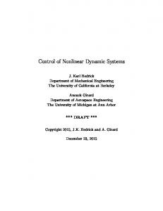
θ x(z)

z Fig. 2.1 Displacement field for the thin-walled beam y s n

rn(s) x a(s) Fig. 2.2 Configuration of a cross-section of a thin-walled beam

19

n

Host structure

Actuator patch

n-(k)

n+(k)

s s+ (k)

s-(k)

Fig. 2.3 Piezoactuator patch distribution n

s

+ + -

z

_ Applied Voltage

+

+ -

+ -

+ -

+ -

Electrode Poling direction

Piezoelectric layer

Fig. 2.4 Piezoelectric layer Nomenclature

20

Dipole

CHAPTER III. STRUCTURAL TAILORING AND ACTIVE CONTROL METHODOLOGIES

3.1 Structural Tailoring Technique As revealed in Chaper 2, the boundary-value problem consists of six differential equations of motion (expressed in terms of the displacements wo ,θ y ,θ x ,uo ,vo and φ ), together with the corresponding BCs. Such a set exhibits a complete coupling between the various modes, i.e., primary and secondary warping, vertical and lateral bending, twist and transverse shear. However, the principal goal of structural tailoring lies in the appropriate selection of fiber orientation so as to produce desired elastic couplings between certain modes. One reason for employing advanced composite materials in flight vehicle design lies in the fact that they permit the use of specific lay-up and fiber orientations so as to induce preferred elastic couplings enhancing the response characteristics. The modified local stiffnesses K12 , K13 , K14 , K24 , K43 defined in Chapter 2 are responsible for producing the elastic couplings. In this sense, there are two well-known configurations, which are shown in Fig. 3.1 and Fig. 3.2 that create unique and special coupling effects. The most general governing equations will be specialized to these structural configurations. 3.1.1 Circumferentially Uniform Stiffness (CUS) Configuration The CUS configuration is characterized by θ(y) = θ(− y) shown in Fig. 3.1. A typical CUS configuration can be described e.g. in terms of ply-angle [θ]n along the entire circumference of the cross section. In this case, the extensional (A), coupling (B) and bending (D) stiffness coefficients are constant at any point on the cross section, which leads to the modified local stiffness relationship Kij (y) = Kij (−y)

(3.1)

For the symmetric biconvex cross section as considered herein, the pertinent geometric conditions to be fulfilled along the circumference of the cross section are as follows: 

dx

∫ x 1, y, ds , F ∫

w

, a  ds = 0,

dx  dy  ds  1, ds , F w, a ds = 0,



dx

∫ y 1, y, ds , F ∫

w

, a ds = 0,

dy  dx  ds  1, ds , F w, a ds = 0,

(3.2a)

∫ ( F , a) ds = 0 w

Substitution of Eqs. (3.1) and (3.2a) into the definitions of stiffeness coefficients aij , yields ten independent stiffness coefficients for the CUS configuration. The direct 21

coefficients are a11, a22 , a33 , a44 , a55 , a66 and a77 , while the coupling ones are a17 , a25 and a34 . Proceeding in a similar way with the mass coefficients, one obtains that b1 , b5 , b10 and b18 are different from zero quantities. Accordingly, in matrix form, the forcedisplacement equations (2.5.4) reduce to: ˆ  Tz  a11  =  Mz   a71    ˆ   My     Mˆ   x    Qx  =   Q   y     Bˆ   w

a17 wo '     a77  φ' 

a 0 0 a25  22   0 a33 a34 0   0 a43 a44 0    a52 0 0 a55  0 0 0  0

0 0 0 0 a66

(3.2b)   θ y'        θ x'      uo' +θy      v o '+θ x     φ" 

(3.2c)

In this case, the governing system and the associated BCs split exactly into two groups; i) Extension-Twist vibrations governed by two coupled equations of the sixth order: ˙˙o , δwo : a11wo "+a17φ"+ pz − Tza ' = b1 w δφ : − a66φ'''' +a71wo "+a77 φ"+mz − Bwa "

(3.3a)

= (b4 + b5 )φ˙˙ − (b10 + b18 )φ˙˙" with the associated BCs at z = 0 : wo = φ = φ' = 0 and at z = L :

(3.3b)

δwo : a11wo ' +a17φ' = 0 , δφ : − a66φ''' +a71wo ' +a77φ' = −(b10 + b18 )φ˙˙' ,

(3.3c)

δφ': a66 φ"= 0 ii) Lateral Bending-Vertical Bending-Transverse Shear vibrations governed by four coupled equations of the eighth order: δuo : a43θ x "+a44 (uo "+θ y ') + px = b1u˙˙o , δvo : a52θ y "+a55 (vo "+θ x') + py = b1v˙˙o , δθ y : a22θ y"+ a25(vo "+θ x' ) − a43θ x' −a44 (uo' +θ y )

22

(3.4a)

+ my − Mya ' = (b5 + b15 )θ˙˙y , δθ x : a33θ x "+ a34 (uo "+θ y ') − a52 θ y ' − a55 (vo ' +θ x ) + mz − Mxa ' = (b4 + b14 )θ˙˙x with the associated BCs at z = 0 : uo = vo = θ x = θ y = 0

(3.4b)

and at z = L : δuo : a43θ x ' +a44 (uo ' +θ y ) = 0 , δvo : a52θ y ' +a55 (v o ' +θ x ) = 0 , δθ y : a22θ y ' +a25 (vo ' +θ x ) = 0 ,

(3.4c)

δθ x : a33θ x ' +a34 (uo ' +θ y ) = 0 But the couplings exhibited by CUS configuration are of no interest for the problem at hand, so that the corresponding problem will not be pursued any further. 3.1.2 Circumferentially Asymmetric Stiffness (CAS) Configuration The CAS configuration is represented by θ(y) = − θ (− y) shown in Fig. 3.2. A typical CAS configuration can be described as a combination of [θ]n along the upper cross section (defined by y >0) and [−θ]n along the bottom cross-section (defined by y Umax u(t) =  −1 T   U max for R W PX (t) rt p

(5.8)

where r denotes the shock pulse length factor and Pm and t p maintain the same meaning as in the case of blast pulses. It may easily be seen that: i) for r = 1 the N-shaped pulse degenerates into a triangular pulse; ii) for r = 2 a symmetric N-shaped pressure pulse is obtained; while iii) for 1< r < 2, as shown in Fig. 5.9(b), the N-shaped pulse becomes an asymmetric one. Another special case emerging from blast and sonic-boom pulses corresponds to a step pulse. The case is obtained from Eq. (5.7), when t p → ∞ and from Eq. (5.8) when r = 1 and t p → ∞ . In addition, the cases of the sine and rectangular pressure pulses described as:  Pm sinπt / tp 0 ≤ t ≤ tp       sine pulse  0 t > tp        py (s, z,t)( ≡ py (t)) =    Pm 0 ≤ t ≤ tp    rectangular pulse    0 t > tp   

54

(5.9)

will considered in the study of the dynamic response. For the problem at hand, only distributed forces will be considered, implying that in the forthcoming developments mz (z,t) = 0 . 5.4 Dynamic Response Control to Blast and Sonic Boom Loadings Herein, a number of successive steps aiming to derive a solution to the dynamic response problem already developed in Chapter 4 will be presented. The virtual work is expressed as L

δW = ∫0 py δvo dz

(5.10)

The system of equations of motion expressed in matrix form (Eq. (4.18)) are rewritten here M* q˙˙(t) + H q˙(t ) + Kq(t) = Q(t)

(5.11)

M *= M + E

where

In state-space form, Eq. (5.11) is written as: X˙ (t) = AX(t) + BQ(t )  0  A=   −M *− 1 K

where

  ,  − M* − 1H 

(5.12a)

0     B =  *− 1  M 

I

(5.12b,c)

Applying Laplace transform to each side of Eq. (5.12a) yields X(s) = (sI − A)−1 X(0) +(sI − A−1 )BQ(s)

(5.13)

where the overbars denote the Laplace transforms of the counterpart quantities without the overbar, X(0) denotes the initial state vector while s denotes Laplace transform variable. The state X(t) is obtained as the inverse Laplace transform of Eq. (5.13):

[

]

X(t) = £ −1 [Φ( s)X(0)] + £ −1 Φ( s)BQ (s)

(5.14a)

Φ(s) ≡ (sI − A)−1

where

(5.14b)

and £ −1 denotes the inverse Laplace transform operation. The top half of the state vector, Eq. (5.14a) can be used in conjunction with Eqs. (4.8) to obtain system responses corresponding to vo , θ x and φ , which are expressed, respectively, as vo (z,t) =

N

∑ϕi (z)qi (t), i =1

θ x (z,t) =

2N

∑ϕ i (z)qi (t),

i = N+ 1

φ(z,t) =

3N

∑ ϕ (z)q (t )

i = 2 N +1

i

i

(5.15)

where ϕ i are space-dependent trial functions and qi are time-dependent generalized coordinates.

55

The following numerical illustrations concern the dynamic response of a cantilevered thin-walled beam incorporating bending-twist coupling, (Eq. (3.6)), as well as of beams featuring transverse-isotropy, (Eq. (3.9)), subjected to time-dependent external excitations. The displayed results correspond to the case of zero initial conditions and of Pm = 500 lbL . In Figs. 5.10-5.14 the dimensionless deflection V˜ (≡ vo L) responses of the beam tip to a sonic boom pressure signature are displayed. Figure 5.10 reveals the efficiency of the tailoring technique to confine the increase of the transverse deflection. From this plot it appears that for θ = 900 , at which the maximum bending stiffness is reached (see Fig. 3.3), a minimum deflection throughout the positive and negative phases of the pulse and even in the free motion range (i.e. for t > rt p when the wave has left the structure) is reached. Figures 5.11 and 5.12 reveal the quantitative and qualitative differences in the response deflection due to a symmetric (r =2), asymmetric (r =1.5) and a degenerated (r =1) sonic boom pulse and due to the positive phase duration of the pulse, t p , respectively. The trends as appearing from these graphs are similar to the ones displayed in Refs. 6 and 7 in the case of a flat panel. In Fig. 5.13 the effects of the transverse shear flexibility of the material of the structure, measured in terms of E G ' is highlighted. Herein E and G' denote the Young's modulus in the plane of isotropy and transverse shear modulus, respectively, where E G ' =0 corresponds to the non-shearable (Bernoulli-Euler) beam model. Whereas during the positive and negative phases of the blast, transverse shear has an almost negligible effect on the deflection, in the free motion range its effect is rather strong and it becomes evident that the classical theory inadvertently underestimates the deflection. The same trend emerges also from Fig. 5.14. In Figs. 5.15-5.16 the effects of a blast load on the response behavior are highlighted. Figure 5.15 which includes the negative phase duration of the blast shows that with the increase of the parameter a' t p lower deflection amplitudes are emerging in the positive phase of the blast. Figure 5.16 highlights the effect of the ply-angle and of the free and constrained warping models on the dynamic response behavior. The results reveal that while the ply-angle plays a significant role in confining the deflection response, for high aspect ratio beams, the warping inhibition plays a negligible role. In Fig. 5.17, the timehistory of the twist angle of the beam tip is recorded. This graph highlights the strong effect played by the tailoring technique towards reducing the twist. Figures 5.18 and 5.19 record the deflection response of the beam to a rectangular pulse. While in Fig. 5.18 the effect of the ply-angles is highlighted, in Fig. 5.19 the effect of transverse shear is displayed. The results in these graphs reveal again the great influence played by the ply-orientation and transverse shear on the transverse deflection response amplitude. The strong influence of transverse shear on deflection amplitude in the free motion range becomes evident also from Fig. 5.19. Figure 5.20 displays the transverse deflection response to a step pulse. In additon to the effect played by the ply-angle, that of the warping restraint emerges clearly from this plot. The results reveal that warping inhibition plays a stronger role in confining the increase of the deflection amplitudes at ply-angles resulting in lower deflection amplitudes. Next, the following obtained results reveal the powerful role played by the dual control methodology mentioned earlier towards enhancing the dynamic response of thinwalled beam cantilevers to various overpressure signatures. In Figs. 5.21 and 5.22 the effects of the dual control methodology on the dynamic response of the beam when subjected to a blast loading are highlighted. In these figures the case of a non-shearable beam free to warp is considered. The results in these plots reveal the strong beneficial influence played by the combined tailoring and adpative technology resulting in a reduction of the deflections in both the forced and free motion ranges. They also reveal that implementation of a ply-angle yielding an increase of the bending stiffness 56

a33 results not only in a dramatic reduction of the deflection in the free motion range, but also in a shift of the deflection peaks towards larger times. A similar conclusion applies when the acceleration feedback control strategy is implemented (see Fig. 5.22). One should remark that within the velocity feedback control methodology, the closed-loop eigenvalues are complex-valued quantities, and as a result, damping is generated. This explains why in the free motion range, for the activated structure and in contrast to the non-activated one, the response amplitudes die out as time unfolds. Incorporation of both velocity and acceleration feedback control strategies results in both a reduction of response amplitude and the shift of their maxima towards larger times. In Figs. 5.23 and 5.24 the open and closed-loop dynamic response to a rectangular pressure pulse are considered. The results reveal that with the increase of the velocity feedback gain, a dramatic reduction of the deflection and twist throughout the forced and free motion ranges, and specially within the latter one, can be achieved. The effect of the warping restraint upon the open and closed-loop dynamic response of the beam subjected to a rectangular pressure pulse is addressed in Fig. 5.25. The results reveal that in the forced motion range, although the warping restraint yields a reduction of the deflection amplitudes as compared with their free warping counterpart, the reduction is not so large as that experienced in the free motion regime. Furthermore, when the beam is activated, for the same feedback gain, the difference of the deflection amplitudes as experienced in the free and constrained warping beam models, are more modest in the free motion regime than in the forced motion regime. In Figs. 5.26 and 5.27 the open and closed-loop dynamic response of cantilevers exposed to a sonic-boom signature are displayed. The results reveal again the powerful effect played by the velocity feedback control in reducing the dynamic deflection amplitude in the forced and free motion regimes. Finally, Figure 5.28 depicts the dynamic response to a sinusoidal pressure pulse. The results from this plot reveal that implementation of the dual control methodology can play a powerful role in controlling the response in both the forced motion range where the tailoring technique plays a more stronger role, and in the free motion range, where the strain actuation technology becomes more efficient. For the sake of implementation of LQR scheme incorporating boundary moment, the non-shearable beam model (Bernoulli-Euler model), Eq. (3.9m), (3.9n,o) and Eq. (3.10c) are used and rewritten here, a33vo '''' +b1 v˙˙o − (b4 + b14 ) v˙˙o "= p y with the associated BCs at z = 0

(5.16)

vo = vo ' = 0

(5.17a,b)

a33vo "= − Mxa , vo ''' = 0

(5.18a,b)

and at z = L

The corresponding discretized equations of motion becomes [M h + M a ] q˙˙ + [K h + K a ]q = [Q] − [F]u

(5.19a)

where M h , M a , K h and K a are the mass and stiffness matrices of the host structure and actuator, respectively, Q is a generalized force vector, while F denotes piezoactuator influence vector.

57

Mh =

∫ [b L

0

h 1

ϕ1ϕ1T − (b4h + b14 h )ϕ 1ϕ 1"T ]dz ,

M a = ∫0 [ b1aϕ 1 ϕ1T − (b4a + b14a )ϕ1ϕ1" T ]dz ,

(5.19b)

L

(5.19c)

L

K h = ∫ 0 a33h ϕ1"ϕ 1"T dz , Ka = Q=

∫

L

0

a33a ϕ1" ϕ 1"T dz ,

(5.20a) (5.20b)

L

∫ϕp 0

1

y

dz

(5.20c)

F = [ϕ1'( L)]

(5.20d)

The corresponding state-space representation of Eq. (5.19a) is where

In addition,

 0 A =  −M − 1K

X˙ (t) = AX (t) + BQ (t) + W u

(5.21)

0   0  I       , B =  −1  and W =   −1 M  −M F  0 

(5.22)

M = Mh + Ma,

K = Kh + Ka

5.5 Influence of Locations and Size of Piezo-Patch Actuators and Sensors Until now, the control based on the piezoactuators spread over the entire beam span, polarized in the thickness direction under an applied electric field ξ 3 (out-of-phase voltage), was considered. However, for evident reasons, piezo-patch actuators are becoming increasingly popular. To illustrate the influence of location and size of a single piezoactuator patch, we consider here the equations of motion for the non-shearable beam model. For this case, the pertinent equation of motion is considered again here − a33 vo "" + py − M ax "= b1v˙˙o − (b4 + b14 )v˙˙o " with the associated BCs at z = 0 and at z = L

vo = vo ' = 0 a33 vo "= 0 , vo ''' = 0

(5.23) (5.24a,b) (5.25a,b)

Symmetric piezoactuator pairs mounted on the thin-walled beam surface (Fig. 5.29) are considered. It should be remarked that the flexural stiffness term a33 includes contributions from both the host structure denoted as a33h , and from piezoactuator patch, denoted as a33a . The latter one is expressed as

58

 A122  2 dx  2   a = ∫   A11 − A  y + D11  ds   R(s, z)ds 11   a 33

(5.26a)

Similarly, the mass terms can be cast in the form b1 = b1h + b1a , b4 = b4h + b4a , b14 = b14h + b14a

(5.26b)

dx (b , b ) = ∫ mo (1, y ) R(s,z )ds , b = ∫ m2  ds  R(s,z)ds

(5.26c)

where 2

a 1

a 4

2

a 14

mo and m2 being associated with the piezoactuator patch, while R(s,z) is a space function defining the distribution in the s and z directions of the piezoactuator. The spatial dependence of the piezoactuator patch for the problem at hand is included explicitly through the piezoelectrically induced moment term Mxa in Eq. (2.5.5b), as l A dx B Mxa = ∫ ∑ ξ3(k ) t a e31(k ) Rk (s, z)  y 1 − A12  + ds  A12 − nak   ds  11 11  k =1

= c R(z )V (t) = cV(t)[ H(z − z1 ) − H(z − z2 )]

(5.27a)

where the Heaviside distribution H(⋅) locates the distributed moment between the points z1 and z2 along the beam span. Using the identity

∫

z2

z1

δ j (z − z ′)h(z)dz = (−1)( j ) h j ( z ′)

(5.27b)

which is valid when z ′ ∈[z1, z2 ] , and that H ′′(z ) = δ ′(z) where δ(⋅) is the spatial Dirac’s distribution, the piezoelectrically induced moment term in the equation of motion Eq. (5.23) is expressed as Mxa" = cV (t)[ δ' (z − z2 ) − δ '( z − z1)] = u [ δ '( z − z2 ) − δ '(z − z1 )]

(5.28)

Therefore, the corresponding piezoactuator influence vector Fi is expressed as Fi = [ϕ i'( z2 ) −ϕ i '(z1 )]

(5.29)

The corresponding discretized equations of motion are expressed as

[ M h + Ma ] q˙˙ + [ K h + K a ] q = Q - [F ]u

(5.30a)

where Mh =

∫ [b ϕ ϕ L

0

h 1

1

T 1

− (b4h + b14h )ϕ1ϕ1" T ] dz 59

(5.30b)

Ma =

∫ [b

Kh =

∫

L

Ka =

∫

z2

z2

z1

0

z1

a 1

ϕ1 ϕ1T − (b4a + b14a )ϕ1ϕ1" T ] dz

(5.30c)

ah33 ϕ1" ϕ1" T dz

(5.30d)

a33a ϕ 1"ϕ1" T dz

(5.30e)

Based on the preceding analysis, numerical simulations were carried out to examine the effects of location and size of piezoactuator patch on the control efficiency. The structure to be controlled according to the LQR scheme is subjected to a blast loading, Eq. (5.7) characterized by Pm = 500 lbL , a' t p = 80 and t p = 0.03 sec . In Fig. 5.30, the variation of the first mode of the damping factor versus location of piezoactuator, expressed in terms of the parameter d (pointing the left end of PZT patch from the clamped end) is displayed. From the figure, one can conclude that when the actuator is located closer to the clamped end of the beam, ζ1 increases, whereas ζ1 decreases as the actuator is located towards the free end of beam. The influence of the location and size of the piezo-patch on the dynamic response of the beam subjected to time-dependent external excitations is considered in Fig. 5.31. From this figure, it becomes apparent that the control efficiency increases dramatically as the patch is located towards the beam root and decays with the increase of the distance from the beam root. In Fig. 5.32 where the dynamic response control of a cantilevered beam under voltage limitation was considered, the effects played by the size and location of a piezopatch on the closed-loop deflection time history of a cantilever subjected again to a blast load are displayed. The result shows that, except for a very short time interval, the boundary bending control resulting when the piezoactuator is spread over the entire beam span, yields almost the same results as the ones occuring in the case of a piezo-patch located near the beam root. In the preceding numerical examples, no limitations upon the control input voltage V(t) has been imposed. However, in realistic problems the depoling voltage of 250 volts in current actuator configuration should be considered as a limitation of piezoactuators. In Fig. 5.33, solid lines correspond to the limited voltage, V max = ± 250volts , while dotted lines correspond to those in which no limitation was considered. From the figure, in spite of the existence of the limitation on V(t), except for several fluctuations of the deflection at the beam tip when subjected to a sonic boom, vibration attenuation appears rather satisfactory. The sensor output voltage is also determined as a function of the sensor position along the beam span when subjected to a triangular pressure pulse. From Fig. 5.34, the sensor voltage is greater in the case of the sensor located near the clamped end, as compared to the case of the sensor located near the free end. This trend can be explained by remarking that the bending moment is larger at the beam root, and as a result, also the strains are larger at that section. In other words, the sensor voltage is greatest for the sensor located at that section where the bending moment is largest. A similar result has been obtained also in Ref. 71. Furthermore, as far as power consumption is concerned, locations of piezoactuator have a large influence on the power requirements during the suppression of the beam vibration. It is found that as the piezoactuator is located towards the root of the beam (i.e. when control effectiveness increases), the power consumption of the piezoactuator increases as well. Fig. 5.35 displays the time history of the power for two cases of the patch location. The maximum power corresponding to the piezoactuator location

60

za = (0.4 − 0.5)L is approximately 33% of the peak value corresponding to the location za = (0.1 − 0.2) L . Figure 5.36 displays the variation of the control force required during the suppression of the beam subjected to the blast load (t p = 0.03sec). It is obvious that as the intensity of blast load is decreases, the control force decreases as well. It is also observed that the maximum magnitude of the control force was 88.8[ lbL ] for the simulated loading conditions and beam configurations (E G' = 0, AR = 6). Finally, in order to assess the effect played by the inclusion of the time-dependent external excitation in the optimal performance index, several test cases are considered. In Fig. 5.37 the response of a clamped thin-walled beam to a blast pulse is displayed. Whereas the control appears to be extremely efficient in damping out vibrations, the difference in the response when the transient load is included or discarded in the optimal performance index is negligible in the free motion regime (i.e. beyond the instant when the pressure pulse has already swept the structure). However, in the forced motion regime, the predictions based on the discard of the pressure pulse in the optimal performance index tend to overestimate the response quantities obtained via their inclusion, by about 10%. One can conclude, consequently, that for a reliable design and control of high performance structures, the time-dependent pulses have always to be included in the performance index. Similar conclusions can also be reached from Figs. 5.38 and 5.39 where the cases of a rectangular and sinusoidal pressure pulses have been considered.

61

0.20

T.S. w/o T.S.

K V=0 K =0.025 V

0.16

0.12

K =0.05

~ V

V

0.08

K V=0.075

0.04

0.00 546.0

551.2

556.4

561.6

566.8

572.0

ω(rad/s) Fig. 5.1 Normalized deflection versus the excitation frequency for AR = 6 and θ = 60o and shearable(T.S.) and nonshearable(w/o T.S.) cantilevers. Warping considered.

10.0 T.S. w/o T.S.

K V=0

8.0

~ V

6.0

K =0.025 V

4.0

K =0.05 V

K =0.075 V

2.0

0.0 76.8

77.1

77.4

77.7

78

ω(rad/s) Fig. 5.2 Normalized deflection versus the excitation frequency for AR = 16 and θ = 60o and shearable(T.S.) and nonshearable(w/o T.S.) cantilevers. No warping considered.

62

0.5

K V=0

0.4

~ V

T.S. w/o T.S.

K V=0.2

0.3

K =0.3 V

0.2

0.1

0.0 228.5

231.4

234.3

237.1

240.0

ω(rad/s) Fig. 5.3 Normalized deflection versus the excitation frequency for AR = 16,θ = 90 o and for shearable(T.S.) and nonshearable(w/o T.S.) cantilevers. No warping considered.

0.20 K =0

T.S. w/o T.S.

V

K =0.025

0.16

V

0.12

φ

K V=0.05 0.08

K V=0.075

0.04

0.00 532

537

542

547

552

557

ω(rad/s) Fig. 5.4 Twist angle versus the excitation frequency for AR = 6,θ = 60o and shearable(T.S.) and nonshearable(w/o T.S.) cantilevers. Free warping model considered.

63

0.20

T.S.

K =0 V

w/o T.S. K V=0.025

0.16

0.12

φ

K =0.05 V

0.08

K V=0.075

0.04

0.00 546

551.2

556.4

561.6

566.8

572

ω(rad/s) Fig. 5.5 Twist angle versus the excitation frequency for AR = 6,θ = 60o and shearable(T.S.) and nonshearable(w/o T.S.) cantilevers. Warping restraint model considered.

1.000 xo=1.0 0.925

x =0.8 o

~ V 0.850

x =0.4 o

0.775 x =0 o

0.700 0

0.00038

0.00075

0.00113

0.0015

KV Fig. 5.6 Normalized deflection versus the feedback gain for AR = 16,θ = 60 o . ( V˜ = V V , V = 2 × 10 5 corresponds to x o =1, KV = 0 )

64

1.0

o

θ=0

0.8

o

θ = 30 0.6

o

θ = 45

~ M

o

θ = 60 0.4

o

θ = 90

0.2

0.0 0

0.001

0.002

0.003

0.004

KV Fig. 5.7 Normalized bending moment at the wing root versus the feedback gain with the ˜ = M M , M = 432583 corresponds to ply-angle as a parameter for AR = 16 ( M o θ = 0 , KV = 0 )

16.0 w/o PZT

KV =0

with PZT 12.0

~ V

K V =0.05 8.0 K V =0.075 4.0

0.0 39.5

41.05

42.6

44.15

45.7

ω(rad/s) Fig. 5.8 Normalized deflection versus the excitation frequency with and without the mass and stiffness of the actuators for AR =16, θ = 0 o .

65

1

a'/tp =0 a'/tp =20 a'/tp =50

py Pm

a'/tp =80

0 tp r tp

Time(s) Fig. 5.9(a) Explosive overpressure signature for various values of a' t p . Negative phase of the pulse included.

1

py Pm

0 tp rt p -1 Time(s) Fig. 5.9(b) Sonic-boom overpressure signature.

66

10.0

θ=0

o

θ=30 θ=90

5.0

~ V

o

o

θ=45

o

0.0 Pm

r tp tp

-5.0

t

p

rt

Free Vibration

p

-10.0 0

0.1

0.2

0.3

0.4

0.5

Time(s)

Fig. 5.10 Influence of ply-angle on time-history of the dimensionless deflection of the beam tip. Sonic-boom overpressure; t p = 0.15 s, r = 1.5, t p = 0.15 s, r = 1.5, Nonshearable and free-warping beam model.

3.0

2.0

r=1.5

r=1.0

1.0

r=2.0 ~ V

0.0 Pm

-1.0

r tp

t

tp

-2.0

tp -3.0 0

0.05

0.1

0.15

0.2

0.25

0.3

Time(s) Fig. 5.11 Influence of the shock pulse length on the time-history of the dimensionless deflection of the beam tip. Sonic-boom overpressure, t p = 0.1 s , AR = 16,θ = 60 o , transverse shear and warping restraint included.

67

3.0

t p =0.25

t p =0.15

tp =0.2

2.0

~ V

1.0

0.0 Pm

-1.0

tp

t r tp

-2.0 0

0.1

0.2

0.3

0.4

0.5

Time(s)

Fig. 5.12 Influence of the positive phase duration of the sonic-boom pulse on the time-history of the dimensionless deflection of the beam tip; r = 1.5 , AR = 16, θ = 60o , transverse shear and warping restraint model.

0.015 tp

Pm

0.010

r tp tp

0.005

~ V

0.000

-0.005

E/G'=0 E/G'=10

-0.010

E/G'=100

r tp

Free Vibration

-0.015 0

0.01

0.02

0.03

0.04

0.05

Time(s)

Fig. 5.13 Effect of transverse shear on time-history of the dimensionless deflection of the beam subjected to sonic-boom pulse, warping inhibition included.

68

0.3 Pm

T.S. w/o T.S

r tp tp

0.15

~ V

0

-0.15

tp r tp

Free Vibration

-0.3 0

0.05

0.1

0.15

Time(s) Fig.5.14 Influence of transverse shear on time-history of the dimensionless deflection of the beam tip subjected to sonic-boom pulse, t p = 0.037 s,r = 2, AR = 6, θ = 45o , Free-warping model.

2.5

a'/tp =0

a'/tp =20

1.37

a'/tp =80 0.25

~ V -0.88

tp

r tp

-2 0

0.05

0.1

0.15

0.2

0.25

0.3

Time(s) Fig.5.15 Influence of parameter a' t p on time-history of the dimensionless deflection of the beam tip; blast pulse, t p = 0.1 s,r = 3, AR = 16, θ = 60o (warping restraint model).

69

6.0 Pm

θ=45o 4.0

θ=60

0.1 t

o

2.0

~ V 0.0

w/o T.S. -2.0 F.W. W.R. -4.0 0

0.1

0.2

0.3

0.4

Time(s) Fig. 5.16 Influence of warping restraint and of the ply-angle orientation on time-history of the dimensionless deflection of the beam tip; blast pulse, t p = 0.1 s,r = 1, AR = 16, nonshearable beam model.

10

tp

θ=30 θ=45

φ

o

θ=60

5

o

o

0 Pm tp

-5

t

T.S. F.W. W.R.

-10 0

0.05

0.1

0.15

0.2

0.25

0.3

Time(s) Fig. 5.17 Influence of ply-angle and warping restraint on the time-history of the twist of the beam tip; blast pulse; t p = 0.1s, AR = 16 shearable beam model.

70

10.0

θ=0

o

θ=45

θ=60

o

o

5.0

~ V

0.0

θ=90 -5.0

o

Pm

0.2

t

-10.0 0

0.1

0.2

0.3

0.4

0.5

0.6

Time(s)

Fig. 5.18 Influence of the ply-angle on time-history of the dimensionless deflection response of the beam tip; rectangular pulse; t p = 0.2s, AR = 16, non-shearable and free warping beam models.

0.015

0.01

~ V

0.005

0

Pm 0.02

-0.005

t

E/G'=0 E/G'=10 E/G'=100

-0.01 0

0.01

0.02

0.03

0.04

0.05

Time(s) Fig. 5.19 Influence of transverse shear on time-history of the dimensionless deflection response of the beam tip; rectangular pulse; t p = 0.02s, AR = 6 , warping inhibition included.

71

6.0

θ=45

5.0

F.W. o

W.R.

θ=60

o

4.0

~ V

3.0 2.0 1.0 Pm

0.0

t -1.0 0

0.1

0.2

0.3

0.4

0.5

Time(s)

Fig. 5.20 Influence of ply-anlge on time-history of the dimensionless deflection response of the beam tip; step pulse; AR = 16, non-shearable beam model

8.0 θ=0

uncontrolled

o o

θ = 45

K V=0.02 4.0

~

V

0.0

-4.0 P

m

0.5

t

-8.0 0

0.5

1

1.5

2

Time(s) Fig. 5.21 Influence of ply-angle on open and closed-loop non-dimensional transverse deflection time-history to a blast loading; t p = 0.5s, AR = 16 , non-shearable and free-warping beam model.

72

7.0 uncontrolled

KA

K V+KA

3.5

~ V

0.0

P

-3.5

m

t

0.4

-7.0 0

0.2

0.4

0.6

0.8

1

Time(s)

Fig. 5.22 Influence of the velocity and acceleration feedback control on the nondimensional transverse deflection time-history to a blast loading. Non-shearable and free warping beam model, θ = 0o , AR = 16, KV = 0.1,K A = 0.005.

3.0 uncontrolled

KV=0.02

KV=0.1

1.5

~

V

0.0

-1.5

P

m

t 0.2

-3.0 0

0.2

0.4

0.6

0.8

1

Time(s) Fig. 5.23 Open and closed-loop non-dimensional transversal deflection time-history to a rectangular pressure pulse. Nonshearable and warping restraint beam model, θ = 0o , AR = 16 .

73

3.0

uncontrolled

F.W. K V=0.05

W.R.

1.5

~ V

0.0

-1.5

Pm

0.3

t

-3.0 0

0.2

0.4

0.6

0.8

1

Time(s)

Fig. 5.24 Free and warping restraint effect on open and closed-loop transverasal deflection time-history to a rectangular pressure pulse. Non-shearable beam model; θ = 60o , AR = 16 .

6.0

P

m

F.W.

rt

p

t

p

W.R.

uncontrolled

K V=0.05

3.0

~ V

0.0

-3.0 tp r tp

Free Vibration

-6.0 0

0.5

1

1.5

Time(s) Fig. 5.25 Free and warping restraint effect on open and closed-loop transverasal deflection time-history to a sonic-boom pressure pulse. Non-shearable beam model; θ = 45o , AR = 16, r = 1.5,t p = 0.15s.

74

5.0

Pm

uncontrolled

rt

p

t

K V=0.1

KV=0.02

p

2.5

~

V

0.0

-2.5 t

p

r tp

Free Vibration

-5.0 0

0.2

0.4

0.6

0.8

1

Time(s) Fig. 5.26 Influence of the velocity feedback gain on the transversal deflection time-history under a sonic-boom pressure pulse. Non-shearable and warping restraint beam model; θ = 45o , AR = 16, r = 1.5,t p = 0.15s.

10.0 uncontrolled

KA

K

V

KV+KA

8.0

6.0

~ V

4.0

2.0

0.0

Pm t

-2.0 0

0.2

0.4

0.6

0.8

1

Time(s) Fig. 5.27 Influence of the velocity and acceleration feedback control on the dimensionless transversal deflection time-history response to a step-pulse. Free warping and non-shearable beam model. θ = 0o , AR = 16, KV = 0.1,K A = 0.005.

75

3.0

2.0 uncontrolled

~ V

KV=0.05

1.0

0.0 o

θ = 45

o

θ = 60 -1.0 0

0.2

0.4

0.6

0.8

1

Time(s)

Fig. 5.28 Influence of the ply-angle and velocity feedback control upon the time-history transversal deflection to a sinusoidal pressure pulse. Non-shearable and warping restraint beam model. AR = 16.

za

sa=3.5"

d

z1

z2 L

Fig. 5.29 Segmented piezoactuator configuration. piezoactuator thickness, t a = 0.00787", spanwise length, L = 30".

76

0.5 a

z =0.1L 0.4

0.3

ζ

1

0.2

0.1

0.0 0.1

0.2

0.3

0.4

0.5

0.6

0.7

0.8

d/L Fig. 5.30 Influence of piezoactuatore patch location on damping factor.

0.010 d=0.8L

0.007

d=0.4L 0.005

d=0.1L

~

V

0.002

0.000

-0.002

-0.005 0

0.01

0.02

0.03

0.04

0.05

Time(s) Fig. 5.31 The effects of location of piezo-patch on the beam tip deflection time history when the beam is exposed to a blast pulse.

77

0.010

0.007

0.005 ~

V

0.002

0.000 za =(0.1-0.2)L za =(0.8-0.9)L -0.002

za =(0.1-0.4)L za =(0 -1)L

-0.005 0

0.0016

0.0032

0.0048

0.0064

0.008

Time(s) Fig. 5.32 Influence of size and location of the piezo-patch on the beam tip deflection time history when the beam is exposed to a blast load. 1 10

5 10

-5

-6

~ V 0 10 0

-5 10 -6 No Limit V max=250 volts w/o Control

-1 10 -5 0

0.02

0.04

0.06

0.08

0.1

0.12

0.14

Time(s) Fig. 5.33 Influence of limitation of control input voltage on transveral nondimensional deflection at the tip of the beam za = (0.1 − 0.2)L .

78

250 za=(0.1-0.2)L

200

a

150 100 50 0 -50 -100 -150 0

0.02

0.04

0.06

0.08

0.1

Time(s) Fig. 5.34 Influence of sensor location on sensor output voltage (triangular pulse, t p = 0.06sec )

15 za=(0.1-0.2)L a

10

Power(watts)

sensor voltages(volts)

z =(0.4-0.5)L

z =(0.4-0.5)L

5

0

-5

-10

-15 0

0.02

0.04

0.06

0.08

0.1

Time(s)

Fig. 5.35 Power consumption variation during suppression of beam vibration subjected to blast load ( Pm = 500

79

lb L ,t p

= 0.06sec ).

0.010

0.008

0.006

Mxa"

0.004 a'/ tp=80 a'/ t =20

0.002

p

0.000

-0.002 0

0.01

0.02

0.03

0.04

0.05

Time(s) Fig. 5.36 Variation of the control force required during suppression of the beam subjected to the blast load. 0.010

0.006

~ V

0.002

-0.002

Pm

0.025

t

-0.006 0

0.01

0.02

0.03

0.04

0.05

Time(s) Fig. 5.37 Influence of the consideration (solid) and discard (dotted) in the performance index of external time-dependent excitation on the beam tip deflection time-history when exposed to a blast loading, AR=6; Solid-dotted line denotes uncontrolled response.

80

0.0100

0.0050

~ V

0.0000

Pm

-0.0050

0.025

t

-0.0100 0

0.01

0.02

0.03

0.04

0.05

Time(s) Fig. 5.38 Counterpart of Fig. 5.37 for the case of a rectangular pressure pulse.

0.006 0.005 0.004 0.003

~ V 0.002 0.001 0.000 -0.001 0

0.01

0.02

0.03

0.04

0.05

Time(s) Fig. 5.39 Counterpart of a Fig. 5.37 for the case of a sinusoidal pressure pulse.

81

CHAPTER VI. CONTROL OF CANTILEVERS CARRYING EXTERNALLY MOUNTED STORES

6.1 Overview The cantilever beams carrying externally mounted stores can serve as a basic model for a number of structures used in the aeronautical, aerospace as well as in other fields of the advanced technology. Civil and military airplane wings are designed to carry heavy external mounted stores along their span. Depending on their magnitude and location, drastic reduction of natural eigenfrequencies and modification of the eigenmodes are experienced [67]. These modifications can result in a deterioration of the dynamic response to time-dependent excitations and can also precipitate the occurrence of the flutter instability [68]. As robot manipulator arms, space booms or antennas operating in space, they are required to be lightweight, strong and of high precision in their mission. Uncontrolled vibration can result in drastic reductions of the accuracy and precision of their operations. In order to control the dynamic response of these structures under time-dependent external excitations and inhibit the damaging effects of vibrations without weight penalties, new technologies have to be implemented. Toward this end, in this chapter a number of results with the vibrational and dynamic response control of cantilevered beams carrying externally mounted stores is addressed. The control mechanism is achieved through the action of a bending moment applied at the tip of the beam. In the forthcoming developments, the theory of cantilevers with external stores incorporating dynamic feedback control capabilities will be addressed and its implications upon their free vibration and dynamic response will be investigated. 6.2 Equations of Motion and Boundary Conditions The case of the cantilevered thin-walled beams of arbitrary closed cross-section is considered. It is assumed that the beam is symmetrically composed of transverselyisotropic material layers (the surface of isotropy in each material layer being parallel to the reference surface of the beam structure). It is assumed that, in addition to a system of concentrated stores of mass m j and mass moment of inertia I j (about their centroid) located at z = z j , ( j = 1, J) , the beam carries also a tip mass of characteristics M and IM . In the case of an airplane wing/robot arm the tip mass can simulate the presence of a tank/payload (Fig. 6.1). Herein J denotes the total number of wing-mounted stores. The equations governing the motion of cantilever beams are established in the context of the following assumptions: i) The cross-sections of the beam do not deform in their own planes. ii) The effects of transverse shear flexibility featured by the advanced composite materials are taken into consideration. iii) The hoop stress resultant Nss is considered negligibly small with respect to the remaining ones. iv) The centroid of the attached masses are distributed along the z-axis.

82

Based upon the previously stipulated assumptions, Hamilton's variational principle [44] extended to the case of a linear 3-D piezoelectric medium can be used to derive the 1D version of the equations of motion and the boundary conditions of adaptive cantilevered beams carrying concentrated masses. However, for the problem considered herein an approximate solution to the electrodynamic problem is postulated with the result that ξ 3 , in the static problem is constant while in the dynamic problem is time dependent. Towards the end of obtaining the governing system of equations, Hamilton's variational principle is used. For the present case, kinetic energy, strain energy and the virtual work associated with the external and dead loads and the piezoelectrically induced boundary moment at the beam tip are expressed, respectively, as follows:  2  ˙ 1 dx ˙  2  ˙ T = 2 ∫τ ρ  v +  yθ x − n ds θ x   dτ   J

[

1 1 + 2 ∑ ∫0 (mj v˙o2 + I jθ˙x2 )δ(z − z j )dz + 2 M v˙o2 + IM θ˙ 2x j=1 L

]

(6.2.1a) z=L

dy 1 L dx dx  V = 2 ∫0 σ zz  yθ x ' −n ds θ x '  + σ sz (v o ' +θ x ) ds  − σ nz (vo ' +θ x ) ds   dz        (6.2.1b) L 1 L = 2 ∫0 [ Mx θ x ' +Qy (vo ' +θ x )] dz = ∫0 [a33 (θ x ' )2 + a55 (vo ' +θ x )2 ] dz J

δW = ∑ ∫ mj gδ (z − z j )δvo dz + ∫ (b1 g − py )δvo dz j =1

L

L

0

0

[

− Mxa δθ x (L,t) + M(g − rM θ˙˙x )δv o − Mr M (˙v˙o + g)δθ x

]

(6.2.1c) z=L

where τ denotes the volume of the 3-D body and g denotes the acceleration of gravity. Following usual steps, the obtained equations of motion in transverse bending are : J   a55 (v o"+θ x' ) −  b1v˙˙o + ∑ m jv˙˙o δ (z − zj ) + py = 0  j =1 

J   a33θ x "− a55( vo ' +θ x ) −  (b4 + b14 )θ˙˙x + ∑ I j θ˙˙x δ(z − zj ) = 0 j=1  

(6.2.2a)

(6.2.2b)

For the beam considered to be clamped at the root and free at the tip, the associated boundary conditions are: vo = θ x = 0 at z = 0 (6.2.3 a,b) and a55 (v o ' +θ x ) + M ˙v˙o − MrM θ˙˙x = 0 (6.2.4 a,b)  at z =L ˙ ˙ a  a33θ x ' + IM θ x − Mr M v˙˙o = M x 

83

In the equations vo (z,t) and θ x (z,t) denote the transverse deflection and rotation about the x − axis, respectively, δ denotes the Dirac's distribution, and a33 and a55 denote the bending and transverse shear stiffness, respectively, which was defined in Eq. (3.9g,h). In addition, rM denotes the offset between the beam extremity and the centroid of the tip mass. The Bernoulli-Euler counterpart of the governing equations (6.2.2) and boundary conditions, Eqs. (6.2.3) and (6.2.4), is obtained through the elimination of a55 (v o ' +θ x ) in Eqs. (6.2.2b), operation followed by consideration of θ x = −vo ' , similarily as in Eq. (3.7). In such a way, the classical equations governing the transverse bending of thinwalled beams carrying concentrated masses are: J J     a33vo '''' − (b4 + b14 )v˙˙o "+ ∑ I j v˙˙o "δ ( z − zj ) +  b1 v˙˙o + ∑ mj v˙˙o δ ( z − zj ) = py  j =1   j =1 

(6.2.5)

while the boundary conditions to be prescribed are: vo = vo ' = 0

at z = 0

  at z =L a33vo "− IM v˙˙o ' + MrM ˙v˙o = Mxa 

(6.2.6 a,b)

a33vo ''' = M ˙v˙o + MrM ˙v˙o '

(6.2.7 a,b)

It should be remarked that both the shearable and non-shearable thin-walled beam models provide fourth order governing equation systems [69]. In Eqs. (6.2.2) and (6.2.3) as well as in Eqn. (6.2.7), the terms identifying the rotatory inertia effect are underscored by a solid line. 6.3 The Control Law For the problem at hand, the piezoelectrically induced boundary moment associated with velocity feedback control law will be used. Within this control law, a proportionality between the moment Mxa at the beam tip and velocity θ˙x (L,t) at the same location is postulated. A more explicit expression of this feedback control law is derived from Eq. (6.2.4b) and is expressed as I Mr k θ x '( L,t) + aM θ˙˙x (L,t) + a M ˙v˙o (L,t) = a v θ˙ x (L,t) 33 33 33

(6.3.1)

where k v denotes the dimensional feedback gain. Related with the bending moment at the beam tip, this can be generated via the use of the converse piezoelectric effect featured with by these devices. In previous chapters it was shown that, in case of piezoactuators spread over the entire beam span, polarized in the thickness direction and featuring in-plane isotropy, under an applied electrical field ξ 3 , a bending moment at the beam tip is generated. For feedback control, the electrical field ξ 3 on which the induced bending moment depends, should be related, through a prescribed functional relationship with the mechanical quantities characterizing the wing's response. In the present case, the established relationship is with the rotational velocity at the beam tip.

84

6.4 Numerical Applications and Discussions For the sake of numerical illustration, the case of a cylindrical thin-walled beam of a biconvex cross-section profile is adopted. The geometry of the cantilevered beam is shown in Fig. 6.1. It is also considered, otherwise stated, that the beam carries a store of mass m1 located along the beam span η(≡ z L) and a tip mass M as well. The beam mass is mb ≡ b1 L , where b1 is the beam mass per unit length. Throughout the numerical illustrations, otherwise stated, it was considered that E G' = 50 , M mb = 0.1, rM = 0.05 L, L = 1 m, b = 0.068 m , t a = 0.2 × 10 −3 m , h = 0.068 m and c = 0.25 m. These dimensions correspond to a beam of aspect ratio, AR = 8 where AR ≡ 2L c . 6.4.1 Free Vibration: Eigenvalue Problem To analyze eigenvalue problem, the external load term has to be discarded and all field variables, generically denoted as F(z,t), have to be represented as F(z,t) = F(z)e λt

(6.4.1)

where λ is the closed-loop eigenvalue. Figure 6.2 displays the influence of a tip mass characterized by the mass ratio α = M mb on the first closed-loop eigenfrequency of a shear deformable beam carrying an uni-store at various locations η(≡ z L) along the beam span. From this plot, it becomes apparent that with the increase of the non-dimensional feedback gain KV (≡ kv Lw a33 ) , the decay of the eigenfrequency resulting from the increase of α and location of the store towards the beam tip can be counteracted. At the same time, the results reveal that with the increase of α , a decay in the efficiency of the control capability is experienced. Herein w (=128.16 rad/s) is the fundamental eigenfrequency of the uncontrolled beam characterized by E G' = 50 and AR = 16 . Figure 6.3 depicts the variation of the first damped eigenfrequency vs. feedback gain KV , for three values of the location of the uni-store and for the shearable and nonshearable beam models. The results reveal that : a) the Bernoulli-Euler beam model (i.e. the model corresponding to E G' = 0) overestimates the frequencies predicted by the actual shearable one and b) the frequencies and control authority diminish with the increase of the distance of the store location, towards the beam tip. The effect of location of the uni-store along the beam span upon the closed-loop first eigenfrequency is highlighted in Fig. 6.4. Herein, the behavior resulting from the consideration of both shearable and non-shearable beam models are illustrated. The results presented in this figure enforce the previously obtained conclusions regarding the influence, on the closed-loop first eigenfrequencies, of transverse shear flexibility and position of the store along the beam span. Figure 6.5 highlights the influence of the distance rM on the first eigenfrequency of the uncontrolled beam. The results obtained from this figure reveal that for small ratios M mb the conclusions in Ref. 85 concerning the negligible influence of rM on the eigenfrequency, are in perfect agreement with the present ones. However, with the increase of the ratio M mb , as is usual in space applications (see Ref. 86), this quantity can play a non-negligible influence on the decay of eigenfrequencies. Figure 6.6 displays the variation of the first mode induced damping ζ1 , as a function of the feedback gain in the case of a beam carrying an uni-store located at different locations. The results reveal that : a) the increase in the induced damping varies almost linearly with the increase of the feedback gain KV , a trend which is consistent with that in

85

Ref. 87. b) The Bernoulli-Euler beam model overestimates the actual damping induced in the shear deformable beam counterpart, overestimation which is exacerbated by the increase of KV and shift of the store toward the beam root. 6.4.2 Steady-State Response to Harmonic Excitations As for the response to persistent harmonic excitations, one considers that the beam is excited by a concentrated harmonically time-dependent load located along the beam zaxis. Hence the load py is represented as py (z,t) = Foδ (z − zo )e iωt

(6.4.2)

where zo ,Fo and ω denote spanwise location of the load, its amplitude and excitation frequency, respectively. Related with the steady state response problem, the variation of the dimensionless steady state response amplitude V˜ (≡ vo L) of the beam tip, for the non-controlled and controlled beam, as a function of the excitation frequency is depicted in Figs. 6.7 and 6.8, where the case of the uni-store of m1 mb = 0.1 and 0.5, respectively, differently located along the beam span is considered. In these plots a shearable beam model is considered. The results reveal : a) the high capability of the control methodology to inhibit/prevent the occurrence of the resonance phenomenon, b) the effect layed by the location of the unistore along the beam span consisting of the shift of the resonance frequency towards larger frequencies when the uni-store is located closer to the beam root and towards lower frequencies when the store is located closer to the beam tip. In Fig. 6.9 the influence of transverse shear flexibility on the steady state deflection amplitude is highlighted. In addition to several of previously outlined conclusions, the results reveal that the classical beam model overestimates the resonance frequency as compared to that occurring in the case of the shearable beam counterpart and that the shift of the location of the store towards the beam tip results in a shift of the resonance frequency towards the lower frequencies. This shift is further exacerbated when, in addition to the uni-store, a tip mass is carried by the beam (see Fig. 6.10). Figures 6.11 and 6.12 display the variation of steady state moment amplitude at the beam root versus the excitation frequency. The results reveal that while the location along the beam span of the uni-store has little effect upon the amplitude of the response, the shift towards lower or larger resonance frequencies (depending on the location of the store toward the beam tip or beam root, respectively) remains the most important effect, in the context of the beam with attached stores or tip mass. In this case, the shift of the resonance frequencies follows the same trend with respect to the ratio m1 mb and the presence of the tip mass, as in the case of the dynamic response deflection amplitude (see Figs. 6.7-6.10). For the sake of completness, Fig. 6.13 presents the variation of the steady-state rotation amplitude θ x vs. the excitation frequency. In this respect, similar conclusions to the ones highlighted by the behaviors of V˜ and M˜ can be outlined in this case, as well.

86

L η

rM

b M mb m1 c

h Fig.6.1 Geometry of the cantilever beam carrying an uni-store and a tip-mass

87

510 K =0.5 v

K =0.3 v

η=0.1

K =0.1 v

d1

ω (rad/s)

473.7

η=0.7

437.5

401.2

η=0.9

365 0.1

0.3

0.5

0.7

0.9

α(=M/m ) b

Fig. 6.2 The first closed-loop eigenfrequency versus the parameter α , for three values of the feedback gain and of the position of the uni-store along the beam span (m1 mb = 0.1) .

640 E/G'=50 E/G'=0

η=0.1

ω d1(rad/s)

572

504

436

η=0.5 η=0.9

368

300 0

0.3

0.6

0.9

KV Fig. 6.3 The first closed-loop eigenfrequency versus the velocity feedback gain, for three options of the uni-store along the beam span and for the shearable and non-shearable beam( M = 0, AR = 8 ).

88

530 Kv =0.3 K =0.2 v

502.5

ω d1(rad/s)

Kv =0.1

475

447.5 E/G'=50 E/G'=0

420 0.1

0.2

0.3

0.4

0.5

0.6

Location of m1(η) Fig.6.4 The first closed-loop eigenfrequency versus the location η of the uni-store, for the shearable and non-shearable and controlled and uncontrolled beam. (m1 mb = 0.5, M = 0, AR = 8) 550 M/m =0.05 b

0.1 500 450

ω 1(rad/s)

0.2 400 350

1.0

300

250 200 0.01

0.02

0.03

0.04

0.05

0.06

0.07

rM /L Fig. 6.5 The first open-loop eigenfrequency versus the dimensionless offset between the beam tip and the centroid of the tip-mass, for four values of the ratio M m b ( E G' = 50, m1 m b = 0.1,η = 0.5).

89

0.2 E/G'=50 E/G'=0

η=0.1 0.15

ζ

1

0.1

η=0.5 0.05

η=0.9

0 0

0.1

0.2

0.3 K

0.4

0.5

V

Fig. 6.6 Induced damping versus the feedback gain, for three values of the uni-store location and shearable and non-shearable beam( m1 mb = 0.5, M = 0, AR = 8) .

0.08 η=0.5

Kv =0

η=0.1

η=0.3

Kv =0.1 0.06

~

V

0.04

Kv =0.2

Kv =0.3 0.02

0 482

487.3

492.5

497.7

503

ω(rad/s) Fig. 6.7 Normalized steady-state deflection amplitude versus the excitation frequency for three locations of the uni-store and for the controlled and uncontrolled beam ( m1 mb = 0.1,M = 0 ).

90

0.09 Kv =0

η=0.3

η=0.1

Kv =0.1 0.06 ~

V Kv =0.2 0.03 K =0.3 v

0 482

487.1

492.3

497.4

502.5

ω(rad/s) Fig. 6.8 Normalized steady-state deflection amplitude versus the excitation frequency for two locations of the uni-store and for the controlled and uncontrolled beam ( m1 mb = 0.5, M = 0 ).

0.08

K =0 v

E/G'=50

K =0.1

E/G'=0

v

0.06

η=0.3

η=0.1

η=0.3

η=0.1

~

V

0.04 K v =0.2 K =0.3 v

0.02

0 492

497

502

507

512

517

522

ω(rad/s) Fig. 6.9 Normalized steady-state deflection amplitude versus the excitation frequency for two locations of the uni-store, for shearable and unshearable beam model ( m1 mb = 0.1,M = 0 ).

91

0.08 η=0.5

K =0

η=0.1

η=0.3

v

K =0.1 v

0.06

~ V

0.04

K =0.2 v

Kv =0.3

0.02

0 470

475.2

480.5

485.7

491

ω(rad/s) Fig. 6.10 Normalized steady-state deflection amplitude versus the excitation frequency for three locations of the uni-store (m1 mb = 0.1,M ≠ 0).

0.3 η=0.3

η=0.1

Kv =0 K =0.1 v

0.2 ~

M

Kv =0.2 0.1

0 481

Kv =0.3

486.75

492.5

498.25

504

ω(rad/s) Fig. 6.11 Steady-state dimensionless root moment amplitude versus the excitation frequency for values of the location of uni-store (m1 mb = 0.5, M = 0 ).

92

0.3

η=0.3

Kv =0

η=0.1

K =0.1 v

0.2 ~ M K =0.2 v

0.1 Kv =0.3

0 472

476.5

481

485.5

490

ω(rad/s) Fig. 6.12 The counterpart of Fig. 6.11 for the case of M ≠ 0 .

0.1 η=0.5

Kv =0

η=0.1

η=0.3

Kv =0.1

0.06 Kv =0.2

x

θ (rad)

0.08

0.04 Kv =0.3 0.02

0 482

487.3

492.5

497.7

503

ω(rad/s)

Fig. 6.13 Steady-state rotation amplitude versus the excitation frequency for three values of the location of the uni-store (m1 mb = 0.1,M = 0).

93

CONCLUSIONS

A dual technology based on the use of structural tailoring and piezoelectric actuation aimed at enhancing the dynamic response characteristics of aircraft wing structures was developed. The results reveal that, using piezoelectrically induced moment control in conjunction with the structural tailoring technique, a significant improvement in the dynamic response of thin-walled cantilever structures can be achieved. This research also highlights the importance of a number of non-classical effects, such as anisotropy, transverse shear and warping restraint, which strongly influence the dynamic response of advanced cantilever structures. Within this study, a study of the control via piezoelectric induced boundary moment and of the moment due to piezoelectric patches was addressed. In addition, optimal control of the response via incorporation of the LQR control and consideration and discard of the external excitation in the performance index was also investigated. Finally, this work addresses also the problem of vibrational and dynamic response control of cantilevers carrying externally mounted stores. The obtained results highlights that the beneficial effect of the application of this dual control methodology, enabling one to modify in a desirable and predictable way the vibration and dynamic response of these structures, as well as to inhibit and even avoid, without weight penalties, the occurrence of the resonance phenonmenon. Although the work addresses mainly the problem of control of aircraft wing structures, the obtained results and developed methods transgress this application in the sense that they can be applied to a number of other structures such as, space booms, flexible robot arms operating in space, etc.

94

REFERENCES

1.

Weisshaar, T.A.,"Aeroelastic Tailoring - Creative Use of Unusual Materials," AIAA Paper 87-0976, AIAA/ASME/ASCE/AHS 28th Structures, Structural Dynamics and Materials Conference, April 9-10, 1987.

2. Librescu, L., Meirovitch, L. and Song, O.,"Refined Structural Modeling for Enhancing Vibrations and Aeroelastic Characteristics of Composite Aircraft Wings," La Recherche Aérospatiale, No.1, 1996, pp. 23-35. 3. Librescu, L., Meirovitch, L. and Song, O., "Integrated Structural Tailoring and Control Using Adaptive Materials for Advanced Aircraft Wings," Journal of Aircraft , Vol. 33, No.1, Jan.-Feb. 1996, pp. 203-213. 4. Rehfield, L.W. and Atilgan, A.R., "Towards Understanding the Tailoring Mechanisms for Thin-Walled Composite Tubular Beams," Proceedings of the First USSR-U.S. Symposium on Mechanics of Composite Materials, 23-26 May, Riga, Latvia SSR, S.W. Tsai, J.M. Whitney, T-W Chou and R.M. Jones (Eds), ASME Publ. House, 1989, pp. 187-196. 5. A.R. Atilgan and L.W. Rehfield,"Vibrations of Composite Thin-Walled Beams with Designed-in Elastic Couplings," Achievements in Composite in Japan and the United States (Ed. A Kobayashi), Tokyo, 1990. 6. D.W. Jensen, E.F. Crawley and J. Dugundji,"Vibration of Cantileverd Graphite/Epoxy Plates with Bending-Torsion Coupling," J. of Reinforced Plastics and Composites, Vol. 1, July, 1982, pp. 254-270. 7.

D.W. Jensen, E.F. Crawley,"Frequency Determination Techniques for Cantilevered Plates with Bending-Torsion Coupling", AIAA J. March, 1984, pp. 415-420.

8. K.B. Lazarus , E.F. Crawley and J.D.Bohlmann, "Static Aeroelastic Control Using Strain Actuated Adaptive Structures," J. of Intelligent Material System and Structures, Vol. 2, pp. 386-410, July 1991. 9. Ehlers, S.M. and Weisshaar, T.A., "Static Aeroelastic Behavior of an Adaptive Laminated Piezoelectiric Composite Wing", Proceeding of the AIAA/ASME/ASCE/ AHS/ASC 31st Structures, Structural Dynamics and Materials Conference, Long Beach, CA, April 1990. 10. Librescu, L. and Song, O., "Behavior of Thin-Walled Beams Made of Advanced Composite Materials and Incorporating Non-Classical Effects," Applied Mechanics Reviews, Vol. 44, No. 11, Part 2, 1991, pp. 174-180. 11. Smith, E.C. and Chopra, I., "Formulation and Evaluation of an Analytical Model for Composite Box-Beams," Journal of the American Helicopter Society, Vol. 36, No. 3, 1991, pp. 23-35.

95

12. L.W. Rehfield, "Design Analysis Methodology for Composite Rotor Blades," Proceedings of the Seventh DoD/NASA Conference on Fibrous Composites in Structural Design, AFWAL-TR-85-3094, v(a)-1-v(a)-15, June 1983. 13. Berdichevsky, V. and Armanios, E. and Badir, A., "Theory of Anisotropic ThinWalled Closed-Cross-Section Beams," Composite Engineering, Vol. 2, Nos. 5-7, pp. 411-432, 1992. 14. Crawley, E.F. and Dugundji, J.,"Frequency Determination and Nondimensionalization for Composite Cantilever Plates," Journal of Sound and Vibration, Vol. 72, No. 1, 1980, pp. 1-10. 15. Kaza, K.R.V. and Kielb, R.E., "Effects of Warping and Pretwist on Torsional Vibration of Rotating beams," Transactions of ASME, Journal of Applied Mechanics, Vol. 51, Dec. 1984, pp. 913-920. 16. J.A. Bowlus, A.N. Palazotto,"Vibration of Symmetrically Laminated Rectangular Plates Considering Deformation and Rotatory Inertia," AIAA J. Vol. 25, No. 11, Nov. 1987, pp. 1500-1511. 17. L.W. Rehfield, A.R. Atilgan and D.H. Hodges, "Nonclassical Behavior of ThinWalled Composite Beams with Closed Cross Sections," J. of the American Helicopter Society, May 1990, pp. 42-49. 18. Timoshenko, S.P., "Vibrations of Bars of Uniform Cross Sections," Philosophical Magazine, Series 6, Vol. 43, 1992, pp. 125-131. 19. Davies, R.M., "The Frequency of Transverse Vibration of a loaded fixed-free bar: IV. The Effects of Shearing of the Bar," Philosophical Magazine, Series 7, Vol. 23, 1937, pp. 1129-1145. 20. Jacobsen, L.S., "Natural frequencies of uniform cantilever beams of symmetrical cross-section," Journal of Applied Mechanics, A-1, Vol. 5, 1938. 21. Mindlin, R.D., "The Influence of Rotatory Inertia and Shear on the flexural motions of isotropic elastic plates," Journal of Applied Mechanics, Vol. 18, 1951, pp. 31-38. 22. Reissner, E., "The Effect of Transverse Shear Deformation on the Bending of Elastic Plates," International Journal of Solids and Structures, Vol. 11, 1975, pp. 569-573. 23. Kruszewski, E.T., "Effects of Transverse Shear and Rotary Inertia on The Natural Frequency of a Uniform Beam," NACA TN-1909, July 1949. 24. Traill-Nash, R.W. and Collar, A.R., "The Effects of Shear Flexibility and Rotatory Inertia on the Bending Vibrations of Beams," Quarterly Journal of Mechanics and Applied Mathematics, Vol. 6, 1953, pp. 186-222. 25. Reissner, E. and Stein, M., "Torsion and Transverse Bending of Cantilevered Plates," NACA TN-2369, June 1951. 26. Peter, A., Stanescu,C. and Librescu, L., "Aeroelastic Divergence of Multicell Wings Taking their Fixing Restraints into Account," Revue de Mecanique Appliquee, Vol. 19, No. 6, 1961, pp. 89-698.

96

27. Librescu, L. and Simovich, J., "General Formulation for the Aeroelastic Divergence of Composite Swept Forward Wing Structures," Journal of Aircraft, Vol. 25, No. 4, 1988, pp. 364-371. 28. A. Gjelsvik, The Theory of Thin Walled Bars , Wiley, New York 1981. 29. Oden, J.T. and Ripperger, E.A., Mechanics of Elastic Structures , McGraw-Hill Book Co., New York, 1980. 30. L.C. Bank and C.H. Kao, "Dynamic Response of Composite Beam," Recent Advances in the Macro- and Micro- Mechanics of Composite Material Structures, AD 13 (D. Hui and J.R.Vinson , Eds.), The Winter annual Meeting of the 1975 ASME, Chicago, Illinois, Nov. - Dec. 1977. 31. W. Lee and H. Chao, "Flexural Vibration Analysis of a Loaded Double-Tapered Circular Beam with a Linearly Varying Wall Thickness," J. Acoust. Soc. Am., 92, (4), Part 1, Oct. 1992, pp. 2260-2263. 32. L. Librescu and A. Nosier, "Dynamic Response of Anisotropic Composite Panels to Time-dependent External Excitations," 17th Congress of the International Council of the Aeronautical Sciences, Paper ICAS 90-1.4R, Stockholm, Sweden, 1990, pp. 2134-2144. 33. E.A. Armanios and A.M. Badir, "Free Vibration Analysis of Anisotropic Thin Walled Closed-Section Beams," AIAA J. Vol. 33, No. 10,Oct. 1995, pp. 1905-1910. 34. Chandra, R. and Chopra, I., "Experimental-Theoretical Investigation of the Vibration Characteristics of Rotating Composite Box Beams," J. of Aircraft, Vol. 29, No. 4, 1992, pp. 657-664. 35. Librescu, L. and Thangjitham, S., "Analytical Studies on Static Aeroelastic Behavior of Forward-Swept Composite Wing Structures," Journal of Aircraft, Vol. 28, No. 2, 1991, pp. 151-157. 36. Lin, C.Y. and Crawley, E.F. "Aeroelastic Actuation Using Elastic and Induced Strain Anisotropy," Journal of Aircraft, Vol. 32, No. 5, Sept-Oct., 1995, pp. 1130-1137. 37. Tzou, H.S., Piezoelectric Shells, Distributed Sensing and Control of Continua, Kluwer Academic Publ., Dordrecht/Boston/London, 1993. 38. Baz, A., "Dynamic Boundary Control of Beams Using Active Constrained Layer Damping," Proc. of the Tenth VPI & SU Symposium, (Etd. Meirovitch), Blacksburg, VA, May 8-10, 1995, pp. 49-64. 39. Librescu, L., Song, O. and Rogers, C.A., "Adaptive Vibrational Behavior of Cantilevered Structures Modeled as Composite Thin-Walled Beams," International Journal of Engineering Science, Vol. 31, No. 5, 1993, pp. 775-792. 40. Tzou, H.S. and Zhong, J.P., Adaptive Piezoelectric Structures: Theory and Experiment , (Ed.) G.J. Knowles, Institute of Physics Publ., 1992, pp. 219-224. 41. Maugin, G.A.,Continuum Mechanics and Electromagnetic Solids, North-Holland, Amsterdam, The Netherlands, 1988.

97

42. Librescu, L., Meirovitch, L. and Na, S.S., "Control of Cantilevers Vibration via Structural Tailoring and Adaptive Materials," AIAA Journal 35(7). 43. Song, O., Modeling and Response Analysis of Thin-Walled Beam Structures Constructed of Advanced Composite Materials , Virginia Polytechnic Institute and State University, Ph.D. dissertation, 1990. 44. Meirovitch, L., Principles and Techniques of Vibrations , Prentice Hall, Englewood Cliffs, 1997. 45. Librescu, L. and Song, O. "On the Static Aeroelastic Tailoring of Composite Aircraft Swept Wings Modeled as Thin-Walled Beam Structures," Composite Engineering 2, 1992, pp. 497-512. 46. Librescu, L. Elastostatics and Kinetics of Anisotropic and Heterogeneous Shell-Type Structures , Noordhoff International, The Netherlands, 1975. 47. Lottati, J., "Aeroelastic Stability Characteristics of a Composite Swept Wing with Tip Weights for an Unrestrained Vehicle," Journal of Aircraft, Vol. 24, No. 11, Nov. 1987, pp. 793-802. 48. Weisshaar, T.A., "Aeroelastic Stability and Performance Characteristics of Aircraft with Advanced Composite Swept Forward Wing Structures," AFFDL-TR-78-118, 1978. 49. O. Song and L. Librescu, "Bending Vibration of Contilevered Thin-Walled Beams Subjected to Time-Dependent External Excitations," J. Acoust. Soc. Am. 98(1), July 1995. 50. Lagnese, J.E. and Lions, J.L., "Boundary Stabilization of Thin Plates," Collection RMA, Masson, Paris, 1988. 51. Lagnese, J.E., "Boundary Stabilization of Thin Plates," SIAM Studies in Applied Mechanics, SIAM, Philadelphia, 1989. 52. Bailey, T. and Hubbard, J.E. Jr., "Distributed Piezoelectric-Polymer Active Control of a Cantilevered Beam," Journal of Guidance, Control and Dynamics, Vol. 8, No. 5, Sept-Oct., 1985, pp. 605-611. 53. Meirovitch, L., Dynamics and Control of Structures , John Wiley & Sons, 1990. 54. Meirovitch, L. and Seitz, T.J., "Structural Modeling for Optimization of Low Aspect Ratio Composite Wings," Journal of Aircraft, Vol. 32, No. 5, 1995, pp. 1114-1123. 55. Wolfram, S., Mathematica, second edition, Addison-Wesley Pub. Co., 1991. 56. Birman, V. and Bert, C.W., "Behavior of Laminated Plates Subjected to Conventional Blast," International Journal of Impact Engineering, Vol. 6, No. 3, 1987, pp. 145-155. 57. Librescu, L. and Nosier, A., "Response of Shear Deformable Elastic Laminated Composite Flat Panels to Sonic Boom and Explosive Blast Loadings," AIAA Journal, 23(2), 1990, pp. 345-352.

98

58. Crocker, M.J., "Theoretical and Experimental Response of Panels to Traveling Sonic Boom and Blast Waves," Wyle Laboratories-Research Staff Report, WR 66-2, 1966. 59. Crocker, M.J., "Multimode Response of Panels to Normal and to Traveling Sonic Booms," The Journal of the Acoustical Society of America, Vol, 42, 1967, pp. 10701079. 60. Crocker, M.J. and Hudson, R.R., "Structural Response to Sonic Booms," J. of Sound and Vibration, 9(3), 1969, pp. 454-468. 61. Crocker, M.J., "Response of Panels to Oscillating and to Moving Shock Waves," J. of Sound and Vibration, 6(1), 1967, pp.38-58. 62. Gupta, A.D., Gregory, F.H. and Bitting, R.L., "Dynamic Response of a Simply Supported Rectangular Plate to an Explosive Blast," Proc. XIII Southestern Conf. on Theoretical and Appl. Mech. 1, 1985, pp. 385-390. 63. Houlston, R., Slater, J.E., Pegg, N. and Des Rochers, C.G., "On the Analysis of Structural Response of Ship Panels Subjected to Air Blast Loading," Computers and Structures, Vol. 21, 1985, pp. 273-289. 64. Gottlieb, J.J. and Ritzel, D.V., "Analytical Study of Sonic Boom From Supersonic Projectiles," Progress in Aerospace Sciences, Vol. 25, 1988, pp. 131-188. 65. R.L. Bisplinghoff and H. Ashley, Principles of Aeroelasticity, Dover Pulblications, INC., 1962 66. E. R. Fleming, "Launch Vehicle Loads," Flight-Vehicle Materials, Structures and Dynamics-Assessment and Future Directions, Vol. 1, New and Projected Aeronautical and Space Systems, Design Concepts and Loads, Sec. 2, New York, 1994, pp. 530541. 67. Abramovich, H. and Hamburger, O., "A Vibration of a Cantilever Timoshenko Beam with a Tip Mass," J. of Sound and Vibration, 148(1), 1991, pp. 162-170. 68. Triplett, W.E., Kappus, H.P.F. and Landy, R.J., "Active Flutter Control-An Adaptable Application to Wing/Store Flutter," J. of Aircraft, Vol.10, 11, 1937, pp. 669-678. 69. O. Song, L. Librescu and C.A. Rogers, "Adaptive Response Control of Cantilevered Thin-Walled Beams Carrying Heavy Concentrated Masses," J. of Intelligent Material System and Structures, Vol. 5, 1994, pp. 42-48. 70. S.M. Yang and Y.J. Lee, "Interaction of Structure Vibration and Piezoelectric Actuation ," Smart Materials and Structures, 3, 1994, pp. 494-500. 71. M-H H. Shen, "Analysis of Beams Containing Piezoelectric Sensors and Actuators," Smart Materials ans Structures, 3, 1994, pp. 439-447. 72. Jeffrey B. Layton, "Flutter Suppression via Adaptive Materials Including Power Consumption," Proc. of the 37th AIAA/SDM Conf. Salt Lake City, UT, April 1996, pp. 1132-1143.

99

73. R. Morris and L. Meirovitch, "Control Algorithm for Flutter Suppression of LowAspect Ratio Composite Wings," Proc. of 10th VPI & SU Symposium on Structural Dynamics and Control (Edt. Meirovitch), Blacksburg, VA, USA, May 8-10, 1995, pp. 275-285. 74. W. K. Belvin and K.C. Park, "Structural Tailoring and Feedback Control Synthesis: An Interdisciplinary Approach," Journal of Guidance, Control and Dynamics, Vol. 13, No. 3, 1990, pp. 424-429. 75. S. M. Yang and C.A. Jeng, "Structural Vibration Suppression by Concurrent Piezoelectric Sensor and Actuator," Smart Materials and Structures, 5, 1996, pp. 806-813. 76. J. Dosch, D. Inman and E. Garcia, " A Self-sensing Piezoelectric Actuator for Collocated Control," J. of Intelligent Material System and Structures, 3, 1992, pp. 166-184. 77. K. Ghosh and R.C. Batra, "Shape Control of Plates Using Piezoceramic Elements," AIAA Journal, Vol. 33, No. 7, July 1995, pp. 1354-1357. 78. M. Sunar and S.S. Rao, "Distributed Modeling and Actuator Location for Piezoelectric Control Systems," AIAA Journal, Vol. 34, No. 10, 1996, pp. 2209-2211. 79. M. Sunar and S.S. Rao, "Thermopiezoeletric Control Design and Actuator Placement," AIAA Journal, Vol. 35, No. 3, March 1997, pp. 534-539. 80. D. E. Kirk, Optimal Control Theory: An Introduction, Prentice Hall, 1970 81. W. L. Brogan, Modern Control Theory, 2nd Ed., Prentice Hall, Inc., 1985 82. A. A. Bolonkin and N. S. Khot, "Optimal Bounded Control Design for Vibration Suppression," Acta Astronautica, Vol. 38, No. 10, 1996, pp. 803-813. 83. N. S. Khot, D. E. Veley and A. A. Bolonkin, "Design of Smart Structures with Bounded Controls," Smart Structures and Materials 1996: Mathematics and Control in Smart Structures, Vol. 2715, 1996, pp.173-182. 84. O. Song and L. Librescu, "Bending Vibrations of Adaptive Cantilevers with External Stores," Int. J. Mech. Sci., Vol. 38, No. 5, 1996, pp. 483-498. 85. M.W.D. White and G. R. Heppler, "Dynamics of Timoshenko Beams with Attached Masses," Dynamics and Control of Structures in Space II, Cranfield Inst. of Technology, U.K. (edt. by C.L. Kirk and R.C. Hughes), Computational Mechanics Publ., Southampton, Boston, 1993, pp. 209-224. 86. R. Kumar, "Vibrations of Space Booms Under Centrifugal Force Field," Canadian Aeronaut. Space Inst. (CASI) Trans., 7, 1974, pp. 1-6. 87. H.S. Tzou, J.P. Zhong and J.J. Hollkamp, "Spatially Distributed Orthogonal Piezoelectric Shells Actuators: Theory and Applications," Journal of Sound and Vibration, 177(3), 1994, pp. 363-378.

100

APPENDIX A

The reduced rigidity quantities are as follows: A2 K11 = A22 − A12 , 11

A A K12 = A26 − 12A 16 = K 21 , 11 A2 K22 = A66 − A16 , 11

A B K14 = B22 − 12A 12 = K41 , 11 K24 = B26 −

A16 B12 A11 = K42 ,

B A K51 = B26 − 16A 12 , 11

K13 = 2K12

AC , β

K23 = 2K22

AC , β

K43 = 2K24

AC , β

B2 K44 = D22 − A12 , 11

K52 = B66 −

B16 A16 A11 ,

K53 = 2K52

AC , β

B B K54 = D26 − 12A 16 11 where Aij , Bij and Dij denote local stretching, stretching-bending coupling and bending rigidity quantities, respectively. The inertia terms are

(

)

(

)

I1 = ∫ u˙˙o − yφ˙˙ mo ds , I2 = ∫ v˙˙o − x φ˙˙ mo ds ,

(

)

˙˙o + xθ˙˙y + yθ˙˙x − Fwφ˙˙' mo ds , I3 = ∫ w I4 =

∫ [( x

2

]

+ y 2 )φ˙˙ − y u˙˙o + x v˙˙o mo ds ,

[

]

˙˙o + x 2θ˙˙y + xyθ˙˙x − xFw (s)φ˙˙' mo ds I5 = ∫ x w

 dy 2  dy dx dy + ∫  ds  θ˙˙y − ds ds θ˙˙x − ds a(s)φ˙˙'  m2 ds ,  

[

]

˙˙o + y 2 θ˙˙x + xyθ˙˙y − yFw (s)φ˙˙' mo ds I7 = ∫ y w

 dx  dx dy dx + ∫   ds  θ˙˙x − ds ds θ˙˙y − ds a(s)φ˙˙'  m2 ds ,   2

[

]

˙˙o − xFw (s)θ˙˙y − yFw (s)θ˙˙x + F w2 φ˙˙' mo ds I9 = ∫ − Fw (s) w

101

dy dx + ∫  ds a(s)θ˙˙x − a(s) ds θ˙˙y + a2 (s )φ˙˙'  m2 ds   where (mo , m2 ) =

N

h (k )

k =1

h ( k− 1)

∑∫

ρ (k ) (1, n2 ) dn

denote the mass terms. The rigidity terms are symmetric, aij = a ji (i, j = 1,7) and have the expressions a11 = ∫ K11ds ,

dy  a12 = ∫  xK11 + K14 ds  ds ,

 a13 = ∫  yK11 − K14 dx ds  ds, dy a15 = ∫ K12 ds ds ,

dx a14 = ∫ K12 ds ds , a16 = − ∫ [ K11 Fw (s) − K14 a(s)] ds ,

a17 = ∫ K13 ds , dy dy dy  a22 = ∫  K11 x 2 + 2x K14 ds + K 44 ds ds  ds , dy  dx dx dy a23 = ∫  K11xy − xK 14 ds + yK14 ds − K 44 ds ds  ds , dy dy dy  dx dx dy  a24 = ∫  xK 12 ds + K24 ds ds  ds , a25 = ∫  x K12 ds + K24 ds ds  ds , dy dy  a26 = − ∫  xK 11F w + xK 14 a + Fw K14 ds + K 44 a ds  ds ,  dy dx dx dx   a27 = ∫  x K13 + K43 ds  ds , a33 = ∫  K11y 2 − 2yK14 + K44 ,  ds ds ds  dy dy dy dx dx dx  a34 = ∫  yK12 ds − K24 ds ds  ds , a35 = ∫  yK12 ds − K24 ds ds  ds , dx dx a36 = − ∫  yK11 Fw + yK 14 a − Fw K14 ds − K44 a ds  ds , dx a37 = ∫  yK 13 − K43 ds  ds ,

dy dy  dx dx a44 = ∫  K 22 ds ds + A44 ds ds  ds

102

 dx dy dx dy a45 = ∫  K22 ds ds − A44 ds ds  ds , dx dx dx a46 = − ∫  Fw K21 ds + K24 a ds  ds , a47 = ∫ K23 ds ds , dy dy dy dy  dx dx  a55 = ∫  K22 ds ds + A44 ds ds  ds , a56 = − ∫  FwK 21 ds + K24 a ds  ds , dy a57 = ∫ K 23 ds ds , a66 = ∫ ( K11 Fw2 + 2K14 Fwa + K 44 a 2 ) ds , a67 = − ∫ ( K13 Fw + K43 a) ds , a77 = ∫ 2

AC K ds . β 23

The reduced mass terms are as follows:

(b1 ,b4 ,b5 ,b10 ) = ∫ mo (1, y 2 , x 2 , Fw2 ) ds, 

 (b14 , b15 , b18 ) = ∫ m2  dx ds  

103

2

2   dy ,  ds  ,a 2  ds . 

APPENDIX B STRUCTURE MODEL DATA

Table B.1 - Properties of Graphite/Epoxy __________________________________ properties Graphite/Epoxy __________________________________ EL (psi) 30e6 ET (psi) 0.75e6 GLT (psi) 0.37e6 GTT (psi) 0.45e6 µ TT 0.25 µ LT 0.25 ρ (lb sec 2 / in 4 ) 14.3e-5 __________________________________ Table B.2 - Properties of Transverse Isotropy Material __________________________________ properties Transverse Isotropy __________________________________ EL (psi) 30e6 ET (psi) 75e5 GTT (psi) 6e5 µ TT 0.25 µ LT 0.25 ρ (lb sec 2 / in 4 ) 14.3e-5 __________________________________ where subscripts L and T denote directions parallel and transverse to the fibers respectively.

104

APPENDIX C PIEZOELECTRIC MATERIAL PROPERTIES

Table C - Physical Properties of PZT-4 _________________________________________ Thickness(in) ta 0.00787 Elastic Coefficients(psi) C11 2.016e7 C12 1.128e7 C13 1.077e7 C33 1.668e7 C44 3.713e6 Piezoelectric Co.(lb/in V) e31 -0.0297 e33 0.0862 e15 0.0725 Poisson Ratio ν 0.31 2 4 Density(lb sec / in ) ρ 7.0135e-4 Electrical Permittivity(Farad/in) ξ 33p 3.048e-10 __________________________________________

105

APPENDIX D The first six normalized eigenmodes of an unactivated cantilevered thin-walled beam in transversal motion. The characteristics of the beam are provided in Fig. 4.1.

1.0 0.8 0.6 0.4 0.2 0.0 0

0.2

0.4

0.6

0.8

1

z/L

Fig. D1 First mode: 0.9088η 2 − 0.4159 η3 − 0.0010256 η4 + 0.00038η5 + 0.0309η6 − 0.00568η 7

1.0 0.6 0.2 -0.2 -0.6 -1.0 0

0.2

0.4

0.6

z/L

0.8

1

Fig. D2 Second mode: 0.3163η2 − 0.50203η3 + 0.00412 η4 − 0.06199 η5 + 0.5967η 6 − 0.5169 η7

106

1.0 0.6 0.2 -0.2 -0.6 -1.0 0

0.2

0.4

0.6

0.8

1

z/L

Fig. D3 Third mode: 0.02067η 2 − 0.05397 η3 + 0.0104 η4 − 0.08375η5 + 0.4966η6 − 0.7341η7

1.0 0.6 0.2 -0.2 -0.6 -1.0 0

0.2

0.4

0.6

z/L

0.8

1

Fig. D4 Fourth mode: 0.00515η 2 − 0.004849 η3 − 0.1317 η4 + 0.4958η5 − 0.7165η6 + 0.4609η 7

107

1.0 0.6 0.2 -0.2 -0.6 -1.0 0

0.2

0.4

0.6

0.8

1

z/L

Fig. D5 Fifth mode: 0.000703η2 + 0.00168η 3 − 0.05903η4 + 0.2797η 5 − 0.5940η 6 + 0.6532 η7

1.0 0.6 0.2 -0.2 -0.6 -1.0 0

0.2

0.4

0.6

z/L

0.8

1

Fig. D6 Sixth mode: −0.003926η2 + 0.04809 η3 − 0.2257η 4 + 0.5303η 5 − 0.6707η6 + 0.4451η7

108

VITA Sungsoo Na was born in May 10, 1963 in Seoul, Korea. He graduated from Korea University with a B.S. in 1986, and a M.S. in 1988, both in Mechanical Engineering. After graduation, he worked as a teaching assistant in the Precision Engineering Department at Korea Advanced Institute Science and Technology (KAIST). While in KAIST, he taught undergraduate courses in CAD/CAM lab and experimental stress analysis. He earned a Ph.D degree in Fall 1997 at the Department of Engineering Science and Mechanics at Virginia Polytechnic Institute and State University, Blacksburg, Virginia. While in Blacksburg, he served as an administrative committee member at Korean Baptist Church for four and a half years as well as the President of Korean Student Association for 1995-1996. Dr. Na is going to join the faculty members of University of Korea Industrial Technology which is located in the city of Ansan, Korea in January 1998. With his wife Dong-Eun Park, he has two daughters, Sangwon and Sang-Yoon.

109