I deal with a position data processing and with a position control of the ..... During this work I am going to implement the Camera module for onboard relative.
CZECH TECHNICAL UNIVERSITY IN PRAGUE Faculty of Electrical Engineering
BACHELOR’S THESIS
Tom´aˇs B´aˇca Control of relatively localized unmanned helicopters
Department of Cybernetics Thesis supervisor: Dr. Martin Saska
Čcskévysoké učcnítee hnie ké v Praze FakLi lta clcktroteeh ni*ká Katedra kyberrretřky
aADÁNí eaKgrÁŘsnÉ pRACE Siudcnt:
Tomáš Eáča
Studijní prCIgram: Kybernetika a nabotika (bakaiářský)
Obor:
R.obotika
Názevtématu:
Řízenívzájemnělclkalizovanýelrbezpilotníchhelikoptér
Fokyny pro Vypracování: Cílem práce je navrhnout a implementovat regulátor pro stabilizaci bezpilotní helikoptéry v definované relativní pozici vzhledem k pohybujícímu se objektu. Systém pro vzájemnou vizuálni lokalizaci letounu a sledovaného objektu dodá vedoucí práce a student jej hardwarově i softwarově integruje do poskytnuté robotické platforrny. Systém umoŽní vznášet se nad lokalizačnímobrazcem, případně jej sledovat, bude-li obrazec umístěn na pozemním robotu nebo dalšíhelikoptéře. Výsledky práce budou ověřeny experimentem s pozemním robotem a helikoptérou, případně s párem dvou helikoptér. Pozemní robot a vůdčíhelikoptéra budou sledovat trajektorie poskytnuté vedoucím práce. 1. lntegrovat modul poskytujícívizuální relativní lokalizaci do platformy MikroKopter.
2. Navřhnout a implementovat regulátor umoŽňující stabilizaci helikoptéry s relativní lokalizací ve zpětné vazbě. 3' Analyzovat vliv pohybu vůdčíhelikoptéry (pozemního robotu) na stabilizaci páru robotů. 4. Analyzavat vliv změny poŽadované relativní pozice robotů na funkci regulátoru. 5. ověřit funkčnost systému na vybraných úlohách robotických formací a rgů
Seznam odborné literatury: Eckert, J.; German, R.; Dressler, F.. On autonomous indoor flights: High-quality real-time iocalization using low-cost sensors" 2012 IEEE lnternational Confenence on Comnnunications (lCC), June 2A12
Vedoueí bakalářské práce: lng. Nlartin Saska' Dr. rer. nat.
Platnost zadáni: do konce zirnního semestru 2arcl2a14
avel Ripka, eSe.
iimír Mařík, DrSc' vedofueí katedry
V Praze cne
1CI.
1.2Ů13
eeee h Technical University in Prague Faculty of Electrical Engineering Departr:rerrt of eyberrreties
BACHELOR PROJECT ASS:GNMENT Stuelcnt:
Tornáš EáČa
Study pr6sramme:
eybernettes ani Roboties
$pee řalEsatřcn:
Robotics
Title of Bae helor Projeet: ecrrtr"oi oí Relatir'eiy Loea|izec Unmannee.Í Hellee piers
Guidelines: The airn of the wor[< is to design and implement a controilen for stabilization of an unmanned helicopter (UAV) in a defined relative position to the moving object. System for the relative visual localization of the UAV and the tracked object will be provided by the thesis supervisor. Student integrates the localization system into the UAV platform. The developed method should enable to follow the localization pattern placed on a ground robot (UGV) or another UAV. The system will be verified with a pair UGV-UAV or UAV-UAV. The leading UAV or UGV will follow trajectories provided by the supervisor. 1. lntegrate the visual relative localization module into the UAV platform MikroKopter. 2. Design and implement a controller that allows stabilizing of the helicopter based on the relative localization in the feedback. 3. Analyze the influence of the leading UAV (UGV) movement on the stabilization of the pair of robots. 4. Analyze the influence of the change of robots'desired relative position on to the pe,.fci'rnarce of the controller. 5. Verify the system peďormance using selected tasks of formation and swarm control
iography/Sou rces : Eckert, J,; German, R.; Eressier, F.. en ai-rtonomous indoorfiights. High-quality real-time localization using low-cost sensors" 2012 IEEE lnternational Conference on Communications (lCC), June 2412 Bi bl
Eaehelor Projeet Supervisor: ing. Martin Saska, Dr. rer. nat.
J
Valid unti!: the end of the winter semester of aeaden"lie year 2Ú13Í2Ú14
!nhL
prof. lng" Vladimír Mařík, DrSe.
Head of Department
ffi
Pr*gi"l*, Jř:nLlal',i 1C, :iJ1-l
j /'/''' lrfg ,É,o1
)
"r'' ,,,t't7 ,' ," '/"
"/rť/--ď'-'ť"p_
'
Pďel Rrpka, CSc Dean
Acknowledgements Firstly I would like to thank to my family for their encouragement and support during my whole studies. Furthermore I thank to my supervisor Martin Saska for his great support throughout this project. I would also like to thank Tom´aˇs Krajn´ık and other people from the IMR group for valuable comments and advice.
Abstract This thesis deals with the integration of the visual relative localization module into the UAV MikroKopter platform. I propose a custom design of a flight control board which handles communication and runs control algorithms. I deal with a position data processing and with a position control of the UAV, relatively to a given pattern image. A series of experiments is presented. It shows the performance of the system under various conditions. I examine the ability to follow a moving target and to change a desired position to the pattern. The final experiment tests the UAV within a heterogeneous formation consisting of aerial vehicles and a ground robot.
Abstrakt Tato pr´ace se zab´ yv´a integrac´ı modulu vizu´aln´ı relativn´ı lokalizace do bezpilotn´ı platformy MikroKopter. Navrhl jsem vlastn´ı ˇreˇsen´ı letov´e ˇr´ıdic´ı desky urˇcen´e pro obsluhu komunikace a v´ ypoˇct˚ u ˇr´ıdic´ıch algoritm˚ u. Zab´ yv´am se zpracov´an´ım dat z lokalizaˇcn´ıho modulu a polohov´ ym ˇr´ızen´ım letounu vzhledem k sledovan´emu obrazov´emu vzoru. Uskuteˇcnil jsem s´erii experiment˚ u, kter´e ukazuj´ı chov´an´ı syst´emu v r˚ uzn´ ych podm´ınk´ach. Zkoumal jsem schopnost letounu sledovat pohybliv´ y c´ıl a mˇenit poˇzadovanou polohu vzhledem k c´ıli. Posledn´ı experiment testuje chov´an´ı bezpilotn´ıho letounu v heterogenn´ı formaci skl´adaj´ıc´ı se z letoun˚ u a pozemn´ıho robotu.
CONTENTS
Contents 1 Introduction 1.1
1
Advantages of multirotor VTOL capable vehicles . . . . . . . . . . . . . .
1
2 Related work
3
3 Hardware overview
4
3.1
MikroKopter platform . . . . . . . . . . . . . . . . . . . . . . . . . . . . .
4
3.2
Custom control board
. . . . . . . . . . . . . . . . . . . . . . . . . . . . .
6
3.3
Camera localization module . . . . . . . . . . . . . . . . . . . . . . . . . .
7
4 Custom control board
8
4.1
Description . . . . . . . . . . . . . . . . . . . . . . . . . . . . . . . . . . .
8
4.2
Board schematic
. . . . . . . . . . . . . . . . . . . . . . . . . . . . . . . .
9
4.3
PCB layout . . . . . . . . . . . . . . . . . . . . . . . . . . . . . . . . . . .
9
4.4
Firmware structure . . . . . . . . . . . . . . . . . . . . . . . . . . . . . . .
10
4.5
PWM and PPM I/O . . . . . . . . . . . . . . . . . . . . . . . . . . . . . .
10
5 Integrating the camera module
11
5.1
Hardware integration . . . . . . . . . . . . . . . . . . . . . . . . . . . . . .
11
5.2
Software integration
. . . . . . . . . . . . . . . . . . . . . . . . . . . . . .
11
5.2.1
Changes in the camera module . . . . . . . . . . . . . . . . . . . .
11
5.2.2
Custom control board . . . . . . . . . . . . . . . . . . . . . . . . .
12
5.2.3
Custom protocol . . . . . . . . . . . . . . . . . . . . . . . . . . . .
12
Communication diagram . . . . . . . . . . . . . . . . . . . . . . . . . . . .
13
5.3
6 System identification
14
6.1
Coordinate system . . . . . . . . . . . . . . . . . . . . . . . . . . . . . . .
14
6.2
Dynamics model . . . . . . . . . . . . . . . . . . . . . . . . . . . . . . . .
14
6.3
The identification data . . . . . . . . . . . . . . . . . . . . . . . . . . . . .
15
6.3.1
Manually controlled flight . . . . . . . . . . . . . . . . . . . . . . .
15
6.3.2
Autonomously controlled flight . . . . . . . . . . . . . . . . . . . .
16
Transfer function from input to angle . . . . . . . . . . . . . . . . . . . . .
16
6.4
i
CONTENTS
6.5
Transfer function from angle to velocity . . . . . . . . . . . . . . . . . . . .
17
6.6
Identifying the z axis system . . . . . . . . . . . . . . . . . . . . . . . . . .
19
6.7
Signal noise . . . . . . . . . . . . . . . . . . . . . . . . . . . . . . . . . . .
19
6.8
Transport lags identification . . . . . . . . . . . . . . . . . . . . . . . . . .
20
6.9
Simulink model . . . . . . . . . . . . . . . . . . . . . . . . . . . . . . . . .
21
7 Control design
22
7.1
Filtering the velocity data . . . . . . . . . . . . . . . . . . . . . . . . . . .
22
7.2
Forward and lateral axes controllers . . . . . . . . . . . . . . . . . . . . . .
23
7.3
Altitude controller . . . . . . . . . . . . . . . . . . . . . . . . . . . . . . .
25
7.4
Tracking the constant reference . . . . . . . . . . . . . . . . . . . . . . . .
25
7.5
Experiment with logging of data . . . . . . . . . . . . . . . . . . . . . . . .
26
8 Influence of the moving reference
27
8.1
Outdoor experiment with 2 UAVs . . . . . . . . . . . . . . . . . . . . . . .
27
8.2
Indoor experiment with 3 UAVs . . . . . . . . . . . . . . . . . . . . . . . .
28
8.3
Experiment with a testing rig . . . . . . . . . . . . . . . . . . . . . . . . .
29
9 Influence of setpoint changes
32
9.1
Influence of the camera view . . . . . . . . . . . . . . . . . . . . . . . . . .
32
9.2
Influence of the setpoint change . . . . . . . . . . . . . . . . . . . . . . . .
32
10 Flying in a heterogeneous formation
34
10.1 Form of the formation . . . . . . . . . . . . . . . . . . . . . . . . . . . . .
34
10.2 Trajectories for the formation . . . . . . . . . . . . . . . . . . . . . . . . .
34
10.3 Experimental details . . . . . . . . . . . . . . . . . . . . . . . . . . . . . .
35
10.4 Evaluation of the experiment
37
. . . . . . . . . . . . . . . . . . . . . . . . .
11 Conclusion
38
Appendix A CD Content
41
Appendix B List of abbreviations
43
Appendix C Custom control board schematic
45
ii
LIST OF FIGURES
List of Figures 1
The MikroKopter UAV [6] . . . . . . . . . . . . . . . . . . . . . . . . . . .
1
2
MK Basicset L4-ME [6]. . . . . . . . . . . . . . . . . . . . . . . . . . . . .
5
3
Flight-Ctrl V2.1 ME stabilization unit [6]. . . . . . . . . . . . . . . . . . .
5
4
The custom control board . . . . . . . . . . . . . . . . . . . . . . . . . . .
6
5
The circular pattern for the relative localization. . . . . . . . . . . . . . . .
7
6
Prototypes of the custom control board. . . . . . . . . . . . . . . . . . . .
8
7
PCB layout of the custom control board. . . . . . . . . . . . . . . . . . . .
9
8
Diagram of a communication between units. . . . . . . . . . . . . . . . . .
13
9
Coordinate system around the quadcopter . . . . . . . . . . . . . . . . . .
14
10
A structure of the quadcopter including the internal stabilization. . . . . .
15
11
17
13
The data for identification of the transfer from φD to φ. . . . . . . . . . . . Comparison of velocities - x˙ and P˙x . . . . . . . . . . . . . . . . . . . . . . The data for identification of the transfer from φ to P˙x . . . . . . . . . . . .
14
Final simulink model of x and y axes. . . . . . . . . . . . . . . . . . . . . .
21
15
Comparison of the x˙ and the Kalman filter output velocity x˙ K . . . . . . . .
23
16
Structure of the x axes controler . . . . . . . . . . . . . . . . . . . . . . . .
24
17
Structure of the model together with controllers . . . . . . . . . . . . . . .
24
18
Control deviations during tracking a constant reference in front of the UAV. 25
19
Control deviations logged by the external camera localization module. . . .
26
20
The first outdoor experiment in the test net. . . . . . . . . . . . . . . . . .
27
21
The second experiment with the AR Drone as a leader. . . . . . . . . . . .
28
22
The testing rig for moving the blob and measuring the UAV’s position. . .
29
23
The testing rig with the UAV. . . . . . . . . . . . . . . . . . . . . . . . . .
29
24
Tracking the sine reference. Amplitude 50 mm, frequency 0.33 Hz. . . . . .
30
25
Simulated tracking of the sine reference. Amplitude 50 mm, frequency 0.33 Hz. 30
26
UAV tracking a constant reference. Distance 1.5 m, altitude aprox. 1 m. . .
31
27
UAV tracking a constant reference with setpoint changes. . . . . . . . . . .
33
28
UAV tracking a constant reference, simulated. Setpoint changes. . . . . . .
33
29
Distance setpoint changes. Setpoint values are identical as were in the experiment. . . . . . . . . . . . . . . . . . . . . . . . . . . . . . . . . . . . .
35
12
iii
18 19
LIST OF FIGURES
30
Two UAVs in a distance of 2 m from the ground robot. . . . . . . . . . . .
36
31
Two UAVs in a distance of 1.1 m from the ground robot. . . . . . . . . . .
36
32
Two UAVs after they passed through the obstacles. . . . . . . . . . . . . .
37
33
Custom control board schematic . . . . . . . . . . . . . . . . . . . . . . . .
45
iv
1
INTRODUCTION
1
Introduction
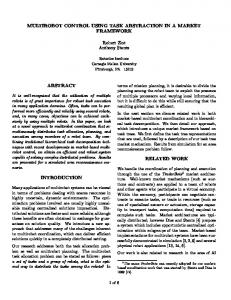
An unmanned aerial vehicle (UAV) is a flying machine controlled either remotely by a human or automatically by an electronic control system. Nowadays VTOL (Vertical Take-Off and Landing) multirotor vehicles are very popular for the case of automatic control [7, 14, 17]. Their main advantage is that there is no need for a large landing ground so they could be easily used between buildings or indoors. There is a couple of types of VTOL capable aircrafts. The common ones are helicopters with one main rotor equipped with variable pitch blades or the multirotor aircrafts such as quadcopters with fixed-pitch propellers. Quadcopter is a VTOL capable aircraft with many advantages compared to other existing UAVs [1]. Thus it fits well for experimental use and especially for indoor flights. These aircrafts utilize fixed-pitch propellers whose thrust depends on a rotational speed. The whole vehicle is controlled only by varying speed of its propellers. There are 2 propellers rotating clockwise and other 2 rotating counter clockwise.
Figure 1: The MikroKopter UAV [6]
1.1
Advantages of multirotor VTOL capable vehicles
• It uses propellers with a fixed pitch angle. • There are significantly less moving parts than the classical helicopter has [1]. • Multirotor aircraft with equivalent power as a helicopter has smaller propellers, thus it is less dangerous due to propeller’s smaller momentum [11]. • It is VTOL capable aircraft. • In most cases it is controlled only by varying propellers speed. It is possible to build a rigid frame without joints and hinges [1]. 1/45
1
INTRODUCTION
On the other hand classical helicopters have significantly more moving and flight critical parts, which makes them inappropriate for experimental use, due to their repair costs. In practice the mechanical complexity of helicopters generates many vibrations which usually disturb cameras and sensors. This makes it inappropriate when it comes to vibration sensitive sensors and it needs special hardware for mounting such sensors. UAV can serve for many purposes which are either dangerous or not feasible for a human. It can explore a building during a fire or search for survivors after some other natural disasters like floods or earthquake. Ground robots are often used for exploring ruins of a building [2, 15]. Aerial vehicles can simply fly over a flooded area and bring information for rescue brigades. There is a need for these vehicles, which is supported by existence of challenges, e.g. DARPA Robotics Challenge [15]. The other natural need is to make these vehicles autonomous. They could operate without a human direct control or they could be able to return to their base after the connection is lost. But every autonomous robot relies on a localization system which tells the robot where it is. In an outdoor environment, the publicly available GPS signal can be used. The GPS provides a satisfactory absolute localization. There is a lot of research being done with GPS localization and it is also very popular among hobbyists. The Paparazzi UAV platform made by ENAC University [18] or the OpenPilot platform [16] are great examples of open-source projects in this area of technology. During this work I am going to implement the Camera module for onboard relative localization in swarm robots [9] into the MikroKopter platform. The camera module is capable of a relative localization of the circular pattern in the view, which is going to be used for automatic control. With the onboard relative localization it should be possible to stabilize the UAV with a constant distance from the tracking object which has the pattern on it. After the pattern is placed on a moving target or other UAV, it should move within a formation with the leading target. The main advantage of the onboard localization approach is the fact that the UAV is able to perform its task not only in laboratory conditions but also in an exterior without the need of external computational power and a precise global localization system. The final goal of this thesis is to conduct a series of experiments which will test capabilities of automatically controlled quadcopters in many different ways. There is an experiment which is designed to find a difference between performance of following a constant reference and a moving reference. Another experiment is going to test the performance of the system when following other UAV equipped with the image pattern. At the end of this thesis, my development of autonomously controlled UAVs is tested. They fly within a formation with a ground vehicle (UGV). The formation is supposed to follow a trajectory, which will be supplied by my thesis supervisor.
2/45
2
2
RELATED WORK
Related work
There is a lot of research in the area of the vision based automatic control of the UAV [11, 17, 10]. Technology of these small electrical aircrafts has been easily accessible for several years since there is a technology of Lithium-Polymer batteries and small embedded electronic with MEMS sensors. Since that time there is a variety of possibilities to obtaion R the UAV. A simple way is to buy the Parrot AR Drone quadcopter which is ready to use due its well behaving embedded system [10]. It is sold as a toy supposed to be controlled by a cellphone. However for the capability of taking an extra payload, people build their custom aircrafts [12] or use some commercially available ones such as Hummingbird [11, 7] or MikroKopter [3] platform. A motion capture system (MoCap) is very popular for tracking UAV’s actual position from the ground [14]. Then a dedicated computer estimates its position and runs control algorithms. Finally control signals are transmitted by wireless to the UAV which follows the computed trajectory. This briefly described method seems to be one trend in this area. There is a research running at the Institute of technology in Zurich that involves a high FPS motion capture system. Their UAVs are able to perform advanced flying maneuvers such as flips [13]. Last year they published interesting results of the quadcopter carrying an inverted pendulum [7] and many other breathtaking experiments. It is considered the state of the art in the area of multirotor UAV. The described method of position measuring has an advantage compared to the relative localization which I use. The measured position (and its derivations) is measured relatively to the ground. A similar research is conducted at the University of Pennsylvania at the GRASP Laboratory [14]. They also use the high FPS MoCap system. Their small quadcopters are able to perform swarm flights with impressive formation changes. But unlike the team at the Institut of technology in Zurich, the GRASP team runs the closed loop controller onboard these flying machines. Only the state estimation process is performed on a dedicated computer. The approach described above relies on the MoCap system which needs to be installed in the room. The room is usually converted into a so called ”testbed” [14]. It provides a safe place both for human and vehicles when the UAV is out of control. A different approach in this area of aerial automation is about an ability to compute and measure all desired values onboard and thus to be able to realize the flight anywhere. Serious challenges are faced during the solution of this task including computing power, inaccurate measurement by the relative localization and others. There is also a research in this area but the tasks are modest at the first sight. The paper [11] describes an approach for landing and position control of a UAV in GPS-Denied environment. In this paper [17], there is an effort to chase a moving target with a UAV localized by an onboard camera. But again, the control loop is realized in a dedicated external computer.
3/45
3
HARDWARE OVERVIEW
3
Hardware overview
There are many ways to obtain a flyable quadcopter. You can build your own. That is the cheapest way. I have a personal experience with building multiple UAVs, from tricopter, quadcopter to hexacopter. But it is very time-consuming and very sensitive to picking and setting up a proper stabilization board, which is essential for flying. Today’s market offers a variety of stabilization platforms [12] and each of them offers a different internal controller. Completely opposite approach it to buy a fully functional device such R as Parrot AR Drone. It provides a very stable flying quadcopter and an open API for development. But its ability to take an extra payload might not be sufficient for taking extra sensors and an onboard computer. The third way is to buy a larger multirotor vehicle prepared for taking much more extra payload. Some of these platforms are suitable for aerial photography such as DJI platform [8] and others are often used for automation e.g. MikroKopter [3] or Hummingbird [11] platform.
3.1
MikroKopter platform
The UAV, employed in this thesis, is a German project MikroKopter, which offers a quadcopter kit. It includes a proprietary stabilization board with open software. When the purchased product is assembled, the UAV acts just like a remotely controlled RC model. It utilizes a standard RC receiver-transmitter set to be able to be armed (activated for flight) and fly under a teleoperation. So it is not very prepared for my purposes of automatic control. The multirotor model that is used in my work is quadrotor MikroKopter M4-LE (Fig. 2). It is a kit which needs to be assembled but all parts are included in the box. Its frame consists of aluminium booms and glass fiber frame plates. The platform utilizes 4 BLDC (Brusless DC) motors equipped with 10” plastic propellers. Two motors rotate clockwise, the other two rotate counter clockwise. Each motor has its own speed controller. These 4 speed controllers are connected via I2 C serial line into a main stabilization board (Fig. 3). The stabilization board sends signals to each BLDC speed controller to obtain the desired motor thrust. It also contains sensors (3-axes gyroscope, 3-axes accelerometer, magnetometer, barometer) and 8-bit AVR MCU for computation. Its main purpose is to stabilize the quadcopter and receive signals from an RC receiver. The MikroKopter platform is well designed so there is no need for an additional tuning of the internal stabilization after it is assembled. But to fly it manually it assumes some experience with the control of at least 4-channel RC helicopter. The control mixing in the stabilization board is set up in a way that it reacts as a very stable coaxial helicopter.
4/45
3
HARDWARE OVERVIEW
Figure 2: MK Basicset L4-ME [6]. The control of such a quadcopter is done by 4 independent signals. The throttle which controls the thrust of all motors, the elevator which controls the forward motion (pitch), the aileron which controls the sideways motion (roll) and the rudder which controls the rotation along the vertical axis (yaw). Because the quadcopter in space has 6 degrees of freedom (DOF) and there are only 4 independent motors, the vehicle is an underactuated system, and thus it is inherently unstable [10, 1] and it needs to be additionally stabilized by some onboard unit.
Figure 3: Flight-Ctrl V2.1 ME stabilization unit [6]. The overall power of this particular machine, which I used, is sufficient for carrying at least 500 g of additional payload. It is powered by 2200mAh 4-cell Lithium-Polymer battery. Total flight time is about 7 minutes and it depends on the weight of payload and character of flying. In addition, the Flight-CTRL provides a battery protection. It can be easily set up and debugged via USB cable using a personal computer.
5/45
3
HARDWARE OVERVIEW
3.2
Custom control board
As mentioned, the employed quadcopter is supposed to be controlled by the RC receiver-transmitter set. In other words, it expects signals from the standard RC receiver. I have designed and built a unit (Fig. 4) which connects the Flight-Ctrl V2.1 ME unit (Fig. 3) and the standard RC receiver. The receiver communicates one-way by pulse-width modulation (PWM). Every channel, which is transmitted, uses one signal wire for PWM at 50 Hz. The custom control board reads every channel with a resolution of 11 bits. Then the control signals are transmitted to the stabilization board using a pulse-position modulation. The custom control board provides two UARTs (Universal asynchronous receiver/transmitter), nine digital inputs for PWM and one digital output for PPM. It can perform basic data processing and simple system controller computation. When the RC set is not used any more, this unit will emulate control inputs such as an arming and a calibration procedure which are currently controlled by the manual controller by a specific input channel combination. The more detail information about the board can be found in chapter 4. The board allows to run control algorithms and when necessary to switch to teleoperated mode. The teleoperator can perform a landing maneuver and prevent an accident.
Figure 4: The custom control board In further development the custom board will also allow to detach the manual RC control completely. It will be undesirable to let the 2.4GHz RC set (that is todays standard in RC hobby) interfere with the Wi-Fi communication, which will be probably used for future swarm control.
6/45
3
HARDWARE OVERVIEW
3.3
Camera localization module
The camera module that was integrated into the MikroKopter platform is a Gumstix TM R R R Overo computer with ARM Cortex A8 processor. The Gumstix has a GNU/Linux operating system installed on, which provides a comfortable access to computer’s hardware along with the Wi-Fi connection. It is supported with a detection software which processes video from an attached camera. The system enables to detect a circular pattern (usually called ”blob”, Fig. 5) in the image and to gather its relative position. The center of the coordinate system is located in the position of the camera.
Figure 5: The circular pattern for the relative localization. The camera module can process the video with resolution of 320×240 px at maximum frame rate 60 Hz and the worst frame rate 33 Hz [9]. It is equipped with one spare UART, which is used for communication with the custom control board.
7/45
4
CUSTOM CONTROL BOARD
4
Custom control board
As mentioned in the previous chapter, the custom control board was made to provide the connectivity for other onboard devices such as RC receiver, camera localization module and MikroKopter flight controller. It also serves as a computational unit for further controller implementation. It was designed from scratch without using an existing microcontroller platform. The custom board is a device for this particular application for control of the multirotor helicopter. It also provides a development on a lower level, which allows to use all native features of the microcontroller, like internal timers and interrupts.
4.1
Description
The whole board is based on the 8-bit AVR ATMega164p microcontroller. Before the board was designed, two prototypes were made, one with ATMega168 and the second with ATMega162 (Fig. 6). The final model (Fig. 4) runs on 18.432MHz clock, provided by an external crystal. The top layer of the board contains the microcontroller, external crystal, two user buttons and two user LEDs, two UARTs, SPI programmer pins, GPIO input and output pins. There are 9 digital inputs intended for connecting to the RC receiver. One digital output for connection to the UAV’s stabilization board and one spare GPIO pin.
(a) 1st prototype
(b) 2nd prototype
Figure 6: Prototypes of the custom control board.
Unlike prototypes, the final model is built of SMD components. There is a USBto-serial FTDI converter placed on the bottom of side the board. It is not used in the proposed application. But if there is a need for connecting the device to the computer via USB, the FTDI can be used easily, instead of connecting an external converter. There are two jumper pins, which can connect the FTDI with the UART0 of the MCU. The pin configuration for PWM and PPM communication is standard with RC hobby components. It is a 3-pin connector with a 5V wire in the middle, GND and signal wire on one side. This configuration provides a protection against accidental polarity reversion. 8/45
4
CUSTOM CONTROL BOARD
The size of the board is 50 × 50 mm with mounting holes compatible with usual stabilization boards. Thus it can be easily mounted above the MikroKopter’s Flight-CTRL stabilization board using 4 spacers. The board is supplied with power from the stabilization board and is able to re-distribute the power to the RC receiver or other component. The software is completely written in C language. When the firmware is compiled using AVR-GCC it can be downloaded into the MCU using any standard SPI programmer, e.g. USBasp.
4.2
Board schematic The complete schematic can be found in Appendix C at the end of this thesis.
4.3
PCB layout
The board was designed as a two-side PCB with top (Fig. 7a) and bottom (Fig. 7b) layers. The main part, including the MCU, is located on the top layer. The design was created using software Eagle. Both sides are protected with solder mask. All components on both sides of the board are labeled using silk screen layer.
(a) The top layer
(b) The bottom layer
Figure 7: PCB layout of the custom control board.
9/45
4
CUSTOM CONTROL BOARD
4.4
Firmware structure
The main() routine executes controller functions and handles interrupt outputs. It also handles buttons, LED’s, debug and other routines like arming/disarming macros. All time-critical actions as communication and control calculations are handled or initiated by interrupts. The main 16-bit timer is used to handle PWM/PPM signal. The other internal 8-bit timer is used to calculate the real time value used for debug and control. All controller functions are executed equidistantly, 70× per second.
4.5
PWM and PPM I/O
The most important part of the firmware is capability to receive PWM channels from the RC receiver and to create a PPM signal for the flight controller. Both signals use periodic (50 Hz) pulses of variable length. This task requires precise time measurement in the MCU. The pulses are standard for RC model electronics. Their length is in interval h1, 2i ms. The measurement needs to be done with precision of tens of µs to achieve the desired resolution. I managed to utilize a single 16bit counter of the MCU to be able to measure simultaneously 9 input PWM channels and to create a PPM signal. There are two compare units with interrupts which are used to create the output PPM signal. The timer itself is clocked by the main clock through the /8 prescaler so it offers a higher-order measurement than the desired precision is (10 µs = 23.04 timer ticks). The incoming PWM signal is measured by storing the time of start and end of every incoming pulse. There is an interrupt hooked for every input pin which executes the proper function to handle PWM pulses.
10/45
5
INTEGRATING THE CAMERA MODULE
5 5.1
Integrating the camera module Hardware integration
The first important task was to mount the device on the quadcopter platform. This was realized by an aluminium frame which holds the camera module bellow the quadrotor frame. Depending on the direction of the camera and whether the camera module is protected with a plastic box (prototype), the aluminium frame is molded to fulfill the desired purpose. Because there is a switching voltage regulator present, the module can be supplied either with its own Li-Po battery or it can be connected directly to the main flight battery. But due to the fact that the main battery lasts only for a few minutes of the flight and then has to be replaced it is preferable to use a separate battery for the camera module. I use 2-cell 2200mAh Li-Po battery. It also lasts longer since the power consumption of the Gumstix computer is relatively small compared to the consumption of the flying quadcopter. According to the supplied hardware documentation of the camera module I connected the UART1 RX, TX and GND pins to TX, RX and GND pins of one of UARTs on the custom control board. The UART settings for this particular communication is: baud rate 57,600 with 8 data bits and one stop bit.
5.2
Software integration
It was necessary to make changes in the software of the camera module and to prepare the custom board for receiving data.
5.2.1
Changes in the camera module
An algorithm that computes the blob’s detection is implemented in the tracker server application (ttracker) [9]. It runs after boot of the Gumstix computer and it waits until a request comes. After that it starts to send a data stream to a client IP address via UDP. So this module can be used also by another computer in the network. I got a source code of a small client application written in C++, which was intended for receiving the data. The tracker client application (tclient) can be run on the same machine as the server and it prints out the data from the tracker server. The tracker client was modified to open the UART1 port, which can be accessed by opening the /dev/ttyS0 device in the OS. When the tclient gets new information it sends it using a custom protocol by writing the message to the ttyS0 file. The message is then sent to the custom control board through the serial line. The tracker client is located in /opt/tracker client/ supplied with a control script that checks whether the client is running. 11/45
5
INTEGRATING THE CAMERA MODULE
Sometimes there was a significant delay between the received data. The delay was caused by an output buffer of the tracker client application. Simple flushing the buffer after each sent message solved the problem. I have made a start up script which controls the tracker client control script. It can start, restart and stop the control script and the tclient depending on the given parameter. The client is always put to background. The script is located in /etc/init.d/ and it has been register for on-boot start up by adding it to the /etc/rc5.d/.
5.2.2
Custom control board
The MCU in the custom control board is the 8-bit ATMega164p made by Atmel. It has two hardware UARTs which can be used separately. The hardware UART activates an interrupt when there is a new byte in the UARTs buffer. The interrupt is handled by a function which has a priority over the main routine of the MCU. After the interrupt function is called, it handles the byte storing it to the buffer in a RAM. Then it is checked, if the buffer contains the whole message from the camera module. If the data matches a correct message, it replaces the particular variable in RAM with the new information from the message. There is also a possibility to send the data in the opposite direction - from the control board to the camera module. This is mostly used for the debugging purpose. The debugging values can be sent in a human readable form and then they can be logged in the Linux machine or the most convenient method is to print them out while being remotely logged in using a ssh session.
5.2.3
Custom protocol
The data from the camera module are sent by a simple custom protocol. At first there is one character that describes which value is following it. These are ’x’, ’y’ and ’z’ for relative distances from the detected pattern and ’v’ for the information about validity of the first three values. The camera module sends the data also in the case when it did not detect any blob. When the data are old (from the last time when the blob was seen) they are followed with the value of ’0’ in the ’v’ variable. All sent values are type of 4-byte integer. Every character at the beginning of the message is followed by 4 bytes of the integer value. After these bytes there is one control byte which is used as an error detection. It is created simply by adding all 5 previous bytes together with the overflow was taken into account. This operation is repeated by the other side of the communication line and when the sum matches the one in the message, it is considered to be correct.
12/45
5
INTEGRATING THE CAMERA MODULE
5.3
Communication diagram
The two-way communication between the stabilization board and the custom control board is realized by the second UART available on the custom control board. For the control design it is necessary to have information about pitch and roll angles in the custom control board. Angles are estimated with the precision of 0.1◦ at the stabilization board. According to [6], the stabilization board uses a custom protocol based on the individual data frames. The data are encoded by modified base64 code. The serial routine of the Flight-CTRL was modified to periodically send values whenever the routine is executed. It led to higher sending frequency than the general firmware offered. I have implemented MikroKopter’s receive and transmit function into the custom control board, so it is able to receive the information about the angle and use it for the control. In the following diagram (Fig. 8) there is a simple communication structure of all electronic components onboard the quadcopter. BL-ctrl v 1.2 BL-ctrl v 1.2 BLDC controller BL-ctrl v 1.2 BLDC controller BL-ctrl v 1.2 BLDC controller BLDC controller
Camera localization module
I2C UART PPM Flight-Ctrl v2.1 ME stabilization board
UART
Custom control board
9x PWM
RC 2.4GHz receiver
Figure 8: Diagram of a communication between units.
13/45
6
SYSTEM IDENTIFICATION
6
System identification
Before the control design, it was necessary to prepare a dynamics model (Fig. 10) of the quadrotor. The model is helpful during the tuning of the controller and it provides useful information about the overall behavior of the system. Using the model, is is possible to simulate the system’s behavior and compare it to experimental results, which is described in chapters 8, 9 and 10.
6.1
Coordinate system
Firstly, it is necessary to define the coordinate system (Fig. 9) in which all values are measured. The center of the coordinate system is located in the camera of the localization module. The quadcopter is (in this case) set in so called ”+” configuration. The x and y axes are parallel to booms of the quadcopter. The z axis is perpendicular to both of them and points downwards. The red color boom signalizes the front of the UAV.
Figure 9: Coordinate system around the quadcopter
6.2
Dynamics model
Because the quadcopter was already equipped with the Flight-CTRL board, the whole system could be identified including the internal stabilization [17, 10]. Because of this, I did not have to model the dynamics of motors, propellers and the other parts to describe the physical nature of the quadcopter. Instead of that, I rely on the Internal stabilization. According to [12], the Flight-CTRL is able to maintain the desired yaw, pitch and roll angles. Based on that, I identified the UAV as a transfer function from desired angles to actual angles which are my state variables. Such quadcopter can be treated as decoupled system [10, 3]. Thus it can be supposed that different axes do not influence each other. In other words it means that each axis can be identified separately. 14/45
6
SYSTEM IDENTIFICATION
Figure 10: A structure of the quadcopter including the internal stabilization.
6.3
The identification data
To assemble the dynamics model it was necessary to obtain the identification data. According to the control system theory it would be desirable to identify the system by measuring e.g. transient response or using other experimental methods described in [5]. But these methods were not used, because this system is unstable, dangerous and easily damageable.
6.3.1
Manually controlled flight
I decided to realize a completely manually controlled flight when the blob was placed bellow the UAV. Therefore the camera on the UAV was pointed to the ground where the blob was placed. In this state the camera module measured the relative position given to the blob. The data were sent to the custom control board which, by that time, had no controller implemented in it. I managed to send periodically all important values from the custom board including control inputs from the RC receiver back to the camera module. There in the camera module the data were logged. I was able to log the data into a ramdisk to increase the writing speed of the logging process.
15/45
6
SYSTEM IDENTIFICATION
According to [10], it is then possible to fit parameters of the dynamics model to the measured data and by doing that to obtain a discrete dynamics model. This flight scenario did not provide the possibility to measure the yaw angle. Actually the camera module does not provide the complete information about the angle of how the camera is pointing the blob. It provides only the unsigned angle between the axes perpendicular to the blob and the axis of the camera. Because of that the yaw part of the system was not identified. All following experiments of this thesis relies on the internal stabilization that is able to hold the constant yaw angle with drift about 5◦ per minute, which can be easily compensated manually by a teleoperator. Following variables were logged during the identification flight: UAV’s positions x, y, z relative to the blob. UAVs pitch and roll angles, control signals pitch, roll, throttle which were sent to the FlightCtrl and time stamp measured by the custom control board. Both the roll and pitch axes were identified together from one set of data. My assumption was that both axes should react in the same way. It was proven by experiments described at the end of this thesis. I have implemented the same controller on both axes, which provides a sufficient results.
6.3.2
Autonomously controlled flight
After I had done the first system identification and control design, I did the data measurement again, but with autonomously controlled UAV above the blob. These data were then used for the system identification again, to obtain better knowledge about the system during its expected behavior. The following presented data are from the second measurement flown by the first implemented controller.
6.4
Transfer function from input to angle
The first transfer function was the one from the control input to the angle of the quadrotor. I directly measured the data vector of desired pitch φ~d and the vector of actual ~ (Fig. 11) so this identification was straightforward. There are two parameters pitch angle φ p0 , p1 , which needed to be identified, assuming it is a first order system. Two vectors φ~d ~ are bound by the following set of linear equations and φ φ(n) = p1 φ(n − 1) + p0 φd (n − 1),
(1)
where n goes from 2 to number of measured data. Constants p0 and p1 are the parameters of the transfer function. The set of equations can be rewritten in the matrix form for all the measured values. It is necessary to obtain an overdetermined system of equations to get sufficient results. 16/45
6
SYSTEM IDENTIFICATION
The matrix form of the set of linear equations is
φ(1) φ(0) φd (0) � � φ(2) φ(1) φd (1) p1 . .. = .. .. . p0 . . φ(n) φ(n − 1) φd (n − 1)
(2)
Parameters p0 and p1 were then found by the least square solution in Matlab. Values of identified parameters are p0 = 0.0221, p1 = 0.9744. Desired and actual pitch angle 4 Desired pitch angle Pitch angle
Angle [deg]
2
0
−2
−4
−6
0
2
4
6
8 10 Time [s]
12
14
16
18
Figure 11: The data for identification of the transfer from φD to φ.
6.5
Transfer function from angle to velocity
The second transfer function from the forward and lateral system part is the angle φ to velocity x˙ transfer. The only difference between the previous and this situation is that I did not directly measure the velocity. Instead of that the position data x were measured and its rate of change was calculated by differentiating its values. Because the position data were noisy so much that its derivation was not usable at all, different approach was chosen. By doing a polynomial fitting to the measured position, the Px polynomial was obtained. The polynomial function was derived and evaluated (Fig. 12). The final least square solution was done with the data of the P˙x . This could be done assuming that the transfer from the velocity to the position is a pure integrator.
17/45
6
SYSTEM IDENTIFICATION Derived position and derived fitted position 30 Derived position Derived fitted position
Velocity [mm/sample]
20 10 0 −10 −20 −30
0
2
4
6
8 10 Time [s]
12
14
16
18
Figure 12: Comparison of velocities - x˙ and P˙x Because the camera was mounted on the moving UAV and pitch and roll angles of the UAV directly influence the measured position, x values needed to be corrected. The data used for identification had already been corrected onboard during the flight using the z coordinate and the angle values. Without these corrections the implemented controller produced bigger oscillations than with them. ~ are As in the previous case (chapter 6.5) the measured data (Fig. 13) vectors ~x, ˙ φ bound by the following set of linear equations. x(n) ˙ = p3 x(n ˙ − 1) + p2 φ(n − 1),
(3)
where n goes from 2 to number of measured data. It can be rewritten in the matrix form for all measured values
x(1) ˙ x(0) ˙ φ(0) � � x(2) ˙ φ(1) ˙ x(1) p3 . .. = .. .. . p2 . . x(n) ˙ x(n ˙ − 1) φ(n − 1)
(4)
~ and vector of velocity For this part of identification I needed a vector of angle values φ values P~˙x . The following set of linear equations is again solved by the least square method. The computed values of parameters are p2 = 0.0058 and p3 = 1.0113.
18/45
6
SYSTEM IDENTIFICATION Pitch angle and forward velocity Angle [deg], Velocity [mm/sample]
10 Pitch angle Forward velocity 5
0
−5
−10
0
2
4
6
8 10 Time [s]
12
14
16
18
Figure 13: The data for identification of the transfer from φ to P˙x .
6.6
Identifying the z axis system
There were attempts to identify the z axis system. None of them had brought a result, which would be useful for simulations. Because of that, the final simulink model (Fig. 17) does not contain the altitude subsystem. The controller used in further experiments was tuned by experimental approach which is discussed in chapter 7.3.
6.7
Signal noise
I calculated the signal noise of measured position x and angle φ by calculating the standard deviation (STD) of these signals. Because these signals are function of time I used the fitted polynomial function as the mean value which is used for the STD calculation. The STD of the position x is calculated by v u n u1 X [xi − pi ], σx = t n i=1
(5)
where n is the number of data values, the ~x is the vector of position values and the p~ is the vector of polynomial values fitted on the ~x. I used the same method for determining the angle values noise σφ as for the position values noise σx . Measured deviations are σφ = 0.8◦ , σx = 5.8 mm. 19/45
6
SYSTEM IDENTIFICATION
6.8
Transport lags identification
Lags of signals were measured to enhance the accuracy of the system model. In the case of the measured angle φ I did not have a method for measuring its transport lag from the time when the quadcopter frame was moved to the time when the custom control board got the information about the movement. But I was able to measure the relative transport lag between the information about the position and the angle value. When the frame is tilted while maintaining the camera position still, the detected blob position changes. It is because of the pattern in the camera image moved. This phenomenon is normally compensated in the custom control board. But without the correct time synchronization of values, the correction would not work well. It creates spikes in position values, when position values are delayed after the angle values. I experimentally found out that the position values from the camera module were delayed behind the angle values from the Flight-CTRL by dmin = 40 ms. I consider this as the lower limit of the position data delay. The next lag I was able to measure was the upper limit of the position data delay, which could be caused by a specific situation. According to [9] the detection algorithm usually do not search over the whole image but it utilizes the previous position of the detection pattern. While the actual position of the the blob is near to the previous position, the detection algorithm is able to hold the FPS at 60 (resolution 320 × 340 px). But when the pattern is lost or its position has changed a lot, the algorithm needs to start from the beginning and it creates a bigger delay than usual. I decided to identify the worst case I was able to came up with. It is the delay between the time when the pattern is not present in the camera image, to the time when the custom control board got the information about the absence of the pattern. I connected LED strips, which were mounted on UAV’s booms, to custom control board, so I was able to switch them off and on. I went with the UAV in the dark place, pointed the camera on the blob and started with the LEDs on, illuminating the blob. And I measured (by the control software) the delay between the time when I had turned the LEDs off and when the board had got the information about the data invalidity. The measured delay was dmax = 160 ms. In the model I use the mean value of these two delays, dmean = 100 ms, as the absolute position delay and the results were consistent with further experiments.
20/45
6
SYSTEM IDENTIFICATION
6.9
Simulink model
The final model (Fig. 14), which is used for simulations, consists of two subsystems – forward and lateral axes. The yaw subsystem is not present because of the lack of the yaw angle data. The altitude subsystem was not successfully identified.
Figure 14: Final simulink model of x and y axes.
21/45
7
CONTROL DESIGN
7
Control design
This dynamics system is useful to test various feedback control techniques such as predictive control, nonlinear control or the simpler ones like state space. I have decided to use the space state controller. My choice is supported by the following facts: I need the controller to be easy computed on the 8-bit AVR processor, considering its support for floating point operation is only emulated. Another reason was, that most of the time I was dealing with the hardware related tasks and data processing and there was not much time for sophisticated control design. The outputs of all following controllers are added to manual control signals with a significant saturation. When testing, the teleoperator can overcome the controllers output to ensure safety for the UAV and its surroundings.
7.1
Filtering the velocity data
The first challenge I faced was the fact that x and y position data were too noisy to use them directly for computing the forward and lateral velocities, as it can be seen in Fig. 12. These data need to be filtered before using them as inputs for the controller. Any filtering technique causing another lag is undesirable, because the bigger the lag is, the more unstable the system seems to be. Because I have the model of the system and I am able to measure another state value (angle) directly, I was able to design a state observer in a form of the Kalman filter. This filtering method causes no additional lag [19] and demands relatively small computational power. In my case the filter estimates the velocity from the angle and then makes a correction by the derived position. Algorithm 1 Kalman filter for forward velocity x˙ K ← 0; x¯˙K ← 0; . Uncertainty of the current velocity value while estimationStep do x˙ E ← p3 · x˙ K + p2 · φ; . Estimation from the pitch angle ¯ ¯ ¯ x˙ K ← x˙ K + x˙ E ; . New uncertainty ¯˙ w ← x¯˙K /(x¯˙K + x); . Computes a weight x˙ K ← (1 − w) · x˙ E + w · x; ˙ . Makes weighted correction ¯ ¯ x˙ K ← (1 − w) · x˙ K ; . New uncertainty end while Constants p2 and p3 are constants from the transfer function of the system. x¯˙K is the variance of the x˙ whose value is 22.3. Because the sequence of w1 , w2 , ..., wn converges over the time, I decided to set it as a constant value 0.15, which had been found experimentally as satisfactory. 22/45
7
CONTROL DESIGN Derived position and Kalman filter output 30 Derived position Kalman filter output velocity Uncorrected estimation from the angle
Velocity [mm/s]
20 10 0 −10 −20 −30
0
2
4
6
8 10 Time [s]
12
14
16
18
Figure 15: Comparison of the x˙ and the Kalman filter output velocity x˙ K . In Figure 15 you can see the filtered velocity from the Kalman filter compared to the x. ˙ There is also uncorrected estimation from the pitch angle. The uncorrected estimation means that it was not corrected by the x, ˙ however the transfer function integration coefficient p3 needed to be slightly modified (by 0.99) to preclude integration out of bound and also a small constant was included to prevent drifting due to angle noise with mean value not equal to zero.
7.2
Forward and lateral axes controllers
I decided to use a state space feedback controller, which in my case consists of three feedback lines. The first one is from the position x, the second one is from the velocity x˙ K and the third one is from the angle φ. Because the system in its essence is a double integrator, such system should not need an additional integration feedback to achieve a zero steady-state error [5]. But only in the case of zero mean value of the noises. Besides the angle value from the stabilization board drifts which causes a major difficulty. The stabilization board itself is not able to achieve the desired angle as the reference angle value drifts by time. It implies into non-zero acceleration when the control input is set to zero. For solving this problem I have implemented the forth feedback line called ”adaptive offset” (Fig. 16). Generally it is an integration feedback but with very limited output (but enough to be able to counter the position drift) and with input equal to sgn xerror . You can see the final structure of the x controller in the Fig. 16 on the following page. All constants were found experimentally with the use of the simulink model and were lately fine tuned during testing the UAV. The same controller is used for both the forward and the lateral axes. 23/45
7
CONTROL DESIGN
Figure 16: Structure of the x axes controler
Figure 17: Structure of the model together with controllers It is very important to distinguish between the setpoint (connected to the controller) and the actual blob’s position (blob is the pattern image used for the relative localization, Fig. 5). Neither the controller nor the localization module do not have the information about the blob’s actual position or velocity. This phenomenon has a very important influence on the system behavior and will be discussed in chapter 8.
24/45
7
CONTROL DESIGN
7.3
Altitude controller
For controlling the altitude I decided to implement a PID controller. Because it is a nonlinear system, some nonlinear adjustments on the controller has to be done, to work properly. Firstly, the gravitational acceleration is eliminated by putting the UAV to the stable state by a manual control. When the controller is turned on, supposing the throttle stick has been left in the position when the UAV flies, the controller does not have to integrate over the whole gravitational acceleration constant. Instead it integrates from the stable point where the UAV was left. But the influence of the gravity persists included in the asymmetric behavior around the stable point. Motors with propellers provide the thrust which pulls the vehicle upwards while the gravity pulls the vehicle downwards. I tested experimentally, that the negative output of the altitude controller needs to be penalized by a coefficient 0.01 and on the other hand the positive output needs to be favored by a coefficient 3. Controller constants were, like in the previous case, found experimentally and they are KP = 0.1, KD = 80, KI = 0.0002.
7.4
Tracking the constant reference
Here I present the time graph of control deviations during a flight when the UAV was tracking a constant reference in front of it. The distance from the blob was set to 1.5 m, the altitude was aprox. 1 m above the ground. Control deviations during a flight
Position deviation [mm]
600 Forward axis deviation Lateral axis deviation Altitude deviation
400 200 0 −200 −400 −600
0
5
10
15
20
25 Time [s]
30
35
40
45
50
Figure 18: Control deviations during tracking a constant reference in front of the UAV.
25/45
7
CONTROL DESIGN
7.5
Experiment with logging of data
Before the last experiment was done, I had discovered a serious issue during the act of measuring the data, presented in the whole thesis. When there is a logging process turned on onboard the Gumstix computer, although the data are being saved on the ramdisk, the process somehow slows down the pattern recognition or it creates another lag. Two experiments were done, while tracking a constant reference - one with data logging onboard the UAV (Fig. 18) and the other one with onboard logging turned off (Fig. 19). In the second case, the position of the UAV was tracked by an external camera localization module facing the UAV which was equipped with the blob. There are the standard deviations of all signals. These two experiments were flown immediately one after the other. STD - internal measurement STD - external measurement
x [mm] 159 85
y [mm] 140 116
z [mm] 123 114
Table 1: Computed STDs Control deviations during a flight measured externally 300 Forward axis deviation Lateral axis deviation Altitude deviation
Position deviation [mm]
200 100 0 −100 −200 −300 −400
0
5
10
15
20
25 Time [s]
30
35
40
45
50
Figure 19: Control deviations logged by the external camera localization module. By comparing Figures 18 and 19 and by comparing standard deviations of the measured data, I assume that the system behavior is significantly worse, when the onboard logging is turned on. So I suppose that all measured oscillations presented in the following experiments are higher than the actual system would have, when no logging would be turned on. The only exception is the Figure 19. The internal logging was intentionally turned off during the flight.
26/45
8
INFLUENCE OF THE MOVING REFERENCE
8
Influence of the moving reference
The position controller has been implemented and the UAV is capable of maintaining constant distance from the pattern image. But there is a difference in the system behavior between the situation when the blob’s position do not change over the time, and when the blob moves. The difference results from the structure of the controller (Fig. 16, 17). The relative position of the quadcopter to the blob is used for x˙ and y˙ velocities estimation. But when the blob is moving, the quadcopter do not have the information about the movement, and the estimated velocities are incorrect. It implies that the action produced by the controller is also inadequate for the current state.
8.1
Outdoor experiment with 2 UAVs
The first experiment was designed to test a capability of the UAV (follower) by letting it follow another UAV (leader). The leader was equipped with the blob and was controlled completely manually by a pilot. There was no special definition of trajectories. The main purpose was to test how the pair of UAVs behaves. The experiment was done outdoors in a testing net, which is built at a courtyard of our faculty.
Figure 20: The first outdoor experiment in the test net. In the enclosed video1 can be seen the UAV pair in the testing net. 1
Video from the first experiment is located in the attached CD or it can be found at the web address http://www.youtube.com/watch?v=0FhWRhw6fhg
27/45
8
INFLUENCE OF THE MOVING REFERENCE
8.2
Indoor experiment with 3 UAVs
Based on the previous experiment, if velocities of the leader were too high, the different type of the UAV should be tested. The following experiment was done with the R Parrot AR Drone quadcopter, which can maintain a very stable hovering state due to its integrated velocity sensor (by computing an optical flow of camera pointing down). The blob was attached to the protection shield of the AR Drone. Two UAVs, equipped with my controller, were placed in the position to form a triangle with the AR Drone. The video2 shows 2 MikroKopter UAVs while following the AR Drone. I assume that wind disturbances produced by ”big” MikroKopter drones caused oscillations of the AR Drone (which is lighter). Followers were not able to follow the leader during most attempts again, but at this time probably because of oscillations of the blob. When the AR Drone was moved manually (by hand) without oscillations, the MikroKopter UAVs followed it smoothly. It implies the main reason of potential instabilities during this experiment were oscillations of the leader. On the other hand the cause of instabilities during the experiment in the testing net, was the speed of the leader, which was too high.
Figure 21: The second experiment with the AR Drone as a leader.
2
Video from the second experiment is also located on the attached CD and on the web address http://www.youtube.com/watch?v=HfCebPWk5Sk.
28/45
8
INFLUENCE OF THE MOVING REFERENCE
8.3
Experiment with a testing rig
My experience with two previously done experiments brought me to the idea to build a device for testing. I have utilized my experience with stepper motor control and I have build a sliding stand to control the blob’s movement. The rig (Fig. 22) was equipped with the camera localization module so it provided an external measurement which can be compared with the internal measurement. The rig was also connected to the custom control board which controlled the blob’s position and processed the data from the camera module. The testing rig provided absolute position of the blob simultaneously with absolute position of the UAV. I decided to measure a UAV’s response to blob’s oscillations to determine how the UAV overshoots the reference. Both following graphs illustrate the lateral axis of the UAV.
Figure 22: The testing rig for moving the blob and measuring the UAV’s position.
Figure 23: The testing rig with the UAV.
29/45
8
INFLUENCE OF THE MOVING REFERENCE
I tried various frequencies of blob’s oscillations with amplitude around 50 mm. In Fig. 24 one illustration example with Amplitude 50 mm and frequency 0.33 Hz is depicted. Big overshoots can be seen, 3× as big as the amplitude of the reference is. The same situation (but different attempt) can be found in the attached video3 . When I simulated the same situation with a simulink model, I got result shown in Fig. 25. UAV tracking moving reference, lateral axis 400 Position of UAV Reference
300
Position [mm]
200 100 0 −100 −200 −300
0
5
10
15
20
25 Time [s]
30
35
40
45
50
Figure 24: Tracking the sine reference. Amplitude 50 mm, frequency 0.33 Hz. UAV tracking moving reference − simulated, lateral axis 400 Position of UAV Reference
300
Position [mm]
200 100 0 −100 −200 −300 −400
0
5
10
15
20
25 Time [s]
30
35
40
45
50
Figure 25: Simulated tracking of the sine reference. Amplitude 50 mm, frequency 0.33 Hz.
3
The video is located on the attached CD and also on web address http://www.youtube.com/watch? v=YD8TeWyAkmk
30/45
8
INFLUENCE OF THE MOVING REFERENCE
For comparison, the tracking of constant reference with two plotted sets of position values is illustrated in the following figure. One is from the testing rig and the other one is from the UAV itself. It can be seen, that the UAV has a distorted information about its position which may cause oscillations. Position sequences were manually synchronized after the measurement. UAV tracking static reference, lateral axis 200 Position of UAV (external) Position of UAV (from UAV) Setpoint
150
Position [mm]
100 50 0 −50 −100 −150 −200
0
5
10
15
20
25 Time [s]
30
35
40
45
50
Figure 26: UAV tracking a constant reference. Distance 1.5 m, altitude aprox. 1 m. Based on first two experiments and measurements with the rig, I assume that the movement of the leading UAV has a significant influence on the stabilization of the following UAV. It may have more than one reason. The first and the main issue of the relative localization is fact, that when the target moves, the UAV follower estimates wrong velocity information. Estimated velocity values do not correspond to the actual velocity relative to the ground (or air). Because of that the UAV behaves differently than if the values were correct. The other source of oscillations and control errors, while following a moving target, could be caused by measurement errors (see for Fig. 26). These errors exist because of tilting of the UAV and because of nonzero yaw angle of the UAV. The yaw angle is manually corrected during the flight, but the correction is not optimal. There are also strong air disturbances caused by the UAV. They may also cause oscillations of the UAV. It can be seen on video from this and the following experiment (chapters 8.3 and 9). The air was even able to lift bulletin boards on the wall. These unknown air conditions may contribute to the overall system behavior and instability.
31/45
9
INFLUENCE OF SETPOINT CHANGES
9
Influence of setpoint changes
The second experiment was realized with the aim to determine the influence of setpoint changes on the UAV’s behavior. There are several aspects of this issue. At first it is a view angle of the camera. In this chapter the UAV was configured to follow the blob placed in front if it. When the UAV is ordered to fly e.g. 500 mm sideways from the blob, the blob is situated not in the center of the camera image. There is a chance that the UAV can fly out of the view of the blob due an overshoot. This situation leads to the end of the flight. The second aspect is the setpoint change itself which may produce overshoots and may destabilize the system.
9.1
Influence of the camera view
The camera view is not square. In the configuration I used during the experiment, the long side of the view was vertical. So it did not offered much space for sideways setpoint changes. The maximal |y| change depends on the distance from the blob. When the UAV is near the blob the maximal lateral setpoint is smaller. Setpoint change of the distance from the blob (x axis) is much more forgiving, than the lateral change. It is limited by the camera view angle, when the UAV is close to the blob. And it is also limited by the camera resolution on the other side. It is possible to fly in distance between 1 m and 2.5 m. The last axis, altitude, is influenced similarly like the lateral axis. With exception that deviation from the center of the view may be slightly bigger than at the lateral axis. It is because this axis takes advantage of the asymmetric camera view.
9.2
Influence of the setpoint change
I took advantage of the measuring rig from the previous experiment and set this experiment up with it as well. The experiment is designed in a similar way. I connected one spare channel of the RC transmitter-receiver as a setpoint switch, which allowed me to change the lateral (y) axis setpoint between two values, 0 and 700 mm. Then I was switching the setpoint during the flight. The UAV’s position was again measured by both the UAV and the measuring rig. The desired distance from the blob was 1.5 m. There are two figures on the following page showing the results. The first one (Fig. 27) shows the measured sequence of the lateral axis position. The second one (Fig. 28) shows the same situation simulated by the simulink model. There is also a video4 from this experiment. The distance from the blob was set to 1.5 m, the altitude was aprox. 1m above the ground.
4
The video is located on the attached CD and also on web address http://www.youtube.com/watch? v=FHSxzy6Md7k
32/45
9
INFLUENCE OF SETPOINT CHANGES UAV tracking static reference with setpoint changes, lateral axis 1000
Position of UAV (external) Position of UAV (from UAV) Setpoint
Position [mm]
800 600 400 200 0 −200
0
10
20
30 Time [s]
40
50
60
Figure 27: UAV tracking a constant reference with setpoint changes.
The Fig. 27 shows that the system did not even touch the setpoint. Despite there was relatively enough time to achieve it. I suppose that it could be caused by the near wall (see attached video). Air, reflected from the wall could have an influence on the control. There was no such phenomenon observed, when the very last experiment was done. See Figure 29 for setpoint changes in forward (x) axis. UAV tracking static reference with setpoint changes − simulated, lateral axis 1000 Position of UAV Reference
800
Position [mm]
600 400 200 0 −200 −400
0
10
20
30 Time [s]
40
50
60
Figure 28: UAV tracking a constant reference, simulated. Setpoint changes.
The simulation showed similar response. Just without such large control error.
33/45
10
FLYING IN A HETEROGENEOUS FORMATION
10
Flying in a heterogeneous formation
Final task in my thesis was to realize an experiment with a heterogeneous formation of multiple robots. The formation was specified by my supervisor. It consisted of 2 UAVs and 1 UGV. Two UAVs were supposed to follow the UGV, one on the left hand side, the other on the right hand side. The formation was meant to follow trajectories supported by the supervisor. The whole experiment was supposed to show an example of use of UAV quadcopters in swarm robotics.
10.1
Form of the formation
The experiment was designed around a big tracked robot which was provided by the IMR (Intelligent and Mobile Robotics) laboratory. I used the aluminium modular system called item, to build a construction on top of the robot. Thus it was possible to mount blobs on it. Two blobs were attached to the sides of the construction, aprox. 0.5 m above the ground. The ground robot provided a platform, capable of smooth and straight ride, controlled from the laptop. The robot was controller by a human operator Two quadcopters were set up so they were able to follow a target located in front of them. Each of them had its own RC set, thus they were both supervised by a human due to safety reasons. During the experiment, these UAVs were located on the sides of the robot, facing the robot. In other words, they both faced each other and the ground robot was located between them. This form of the formation offers a good possibility to change a setpoint of distance from the blob. The UAV is capable of maintaining the position in distance between 1 m and 2.5 m. This is limited by the camera that is used. UAVs were meant to fly in a height of aprox 0.3 m above the blob (0.8 m above the ground), which was enough to eliminate the air ground effect while maintaining the blob in the view of the camera. I prepared both UAVs for the experiment so they were able to change the distance setpoint depending on time. This was a simple way to achieve coordinated movements without any additional communication between robots.
10.2
Trajectories for the formation
The supplied trajectories for the formation were provided by the supervisor. They were, in fact, product of a bachelor’s thesis of my college, Vojtˇech Spurn´ y. His thesis is about planing of formation trajectories. I cooperated with him to obtain distance values, parameterized by time. After a discussion with the supervisor, I decided to transform the trajectory into piecewise linear trajectory due to implementation difficulties. The response of one UAV to planned setpoint changes is shown in the Figure 29. 34/45
10
FLYING IN A HETEROGENEOUS FORMATION
This measurement was realized in a separate experimental run. The plotted response does not correspond with the video from the experiment, due to measurement issue, discussed in the chapter 7.5. The planned velocity of the ground robot was 10 cm/s, so the total traveled distance of the formation was aprox. 4 m. UAV tracking static reference, forward axis 2400 Position of UAV Reference
2200
Position [mm]
2000 1800 1600 1400 1200 1000 800
0
5
10
15
20 Time [s]
25
30
35
40
Figure 29: Distance setpoint changes. Setpoint values are identical as were in the experiment.
10.3
Experimental details
Both UAVs had the same firmware, containing the trajectory, or in other words, the time dependent values of the blobs distance. At first, they were manually placed in the self-stable position. Then, simultaneously, both pilots switched a control switch on the RC transmitter, restarting the internal clock timer in the UAV. Both UAVs started to follow the distance time series. In this time, also the ground robot’s pilot commanded the UGV to move. The ground robot itself was moving independently on UAVs. There was no explicit communication between these vehicles. At first it was tested, that both UAV, act correctly. After the successful testing, two obstacles were placed in the collision course of UAVs. UAVs were meant to utilize the change of the distance from the ground robot, from 2 m to 1.1 m, to avoid the collision. Obstacles were already part of the map used during the planning. There was no feedback either from UAVs nor from the ground robot. This video5 shows two successful attempts of the experiment. The track also contains a rendered simulation of the experiment, supplied by Vojtˇech Spurn´ y, whose also helped during filming of this experiment. 5
The video is located on the attached CD and also on web address http://www.youtube.com/watch? v=Xo2Q_WgXl0A
35/45
10
FLYING IN A HETEROGENEOUS FORMATION
Following photos are from the attempt which can be seen as the second one in the video. There is a pair of UAVs before distance setpoint was changed (Fig. 30). Actual distance from the UAV to the ground robot was aprox. 2 m. The ground vehicle was moving in the direction of the camera view with the velocity of 10 cm/s.
Figure 30: Two UAVs in a distance of 2 m from the ground robot.
In the Figure 31, there is the pair of UAVs just between two obstacles, after the distance setpoint change was made. The actual distance from the UAV to the ground robot was aprox. 1.1 m. Two obstacles were placed in this place a posteriori after the testing was done. There was no feedback control for collision avoidance. Obstacles serve only for illustration purposes to demonstrate behavior of the formation trajectory planning.
Figure 31: Two UAVs in a distance of 1.1 m from the ground robot.
36/45
10
FLYING IN A HETEROGENEOUS FORMATION
The following photo (Fig. 32) shows both UAVs after they passed through the obstacles. Their relative distance to the ground robot was again set to 2 m. The formation continued in the direction of the camera view.
Figure 32: Two UAVs after they passed through the obstacles.
The whole sequence can be seen in the attached video. This particular situation illustrated by Fig. 30, 31 and 32 is presented as the second attempt in the video. In the first part of the video, one of the UAVs has significantly lower altitude than the other. It could be caused by the integration part of the altitude controller. The integrator could have been in the saturation because of poorly set throttle on the RC transmitter (controller’s outputs are added with transmitter outputs, see chapter 7).
10.4
Evaluation of the experiment
The presented experiment showed two UAVs following one ground vehicle. The formation formed by these vehicles changed its shape during passing between two obstacles (without a feedback collision avoidance). Movement of UAVs was time-synchronized. I consider this experiment as successful. It showed, that these relatively localized UAVs can be used in heterogeneous formation together with a ground robot, despite of results of previously done experiments (chapter 8). Considering the experiments, the blob should not be placed on a target vehicle, whose position oscillates or moves with high velocities (more than 40 cm/s).
37/45
11
11
CONCLUSION
Conclusion
This project was a great opportunity to design, develop and test a device which made the UAV autonomous. I have integrated the module for relative visual localization into the MikroKopter UAV platform. I have built a custom control board and realized the position controller in it. The custom board successfully served for communication between other electronics and for the control of the UAV. The UAV was then able to track the position of the recognition pattern. I have tuned the system, so it was able to be tested by various experiments. The first experiments with moving targets showed, that the system’s stability is very affected by the target’s movement. The system worked much better when the target was static. This issue could be eliminated by implementing a sensor for measuring velocity relative to the ground, similar to the one that the AR Drone is equipped with. The overall stability of the system could be enhanced by implementing a different structure of the controller, e.g. the cascade structure. Other experiments shown how the system reacts to setpoint changes. The ability to change the relative position of the UAV given to its target is mostly limited by the camera module. Changes of the setpoint were used during the last experiment, which included two UAVs and one UGV. The experiment shown these vehicles moving in a heterogeneous formation and conduction a change of its shape. All experiments were captured on videos which are provided on the enclosed CD.
38/45
REFERENCES
References [1] Samir Bouabdallah, Pierpaolo Murrieri, and Roland Siegwart. Design and control of an indoor micro quadrotor. In Robotics and Automation, 2004. Proceedings. ICRA’04. 2004 IEEE International Conference on, volume 5, pages 4393–4398. IEEE, 2004. [2] Angela Davids. Urban search and rescue robots: from tragedy to technology. Intelligent Systems, IEEE, 17(2):81–83, 2002. [3] Juergen Eckert, Reinhard German, and Falko Dressler. On autonomous indoor flights: High-quality real-time localization using low-cost sensors. International Conference on Communications (ICC), 2012. [4] Isabelle Fantoni and Rogelio Lozano. Non-linear control for underactuated mechanical systems. Springer, 2001. [5] Gene F Franklin, J David Powell, and Abbas Emami-Naeini. Feedback control of dynamics systems. Pretince Hall Inc, 1986. [6] HiSystems GmbH. Mikrokopter - shop. http://www.mikrocontroller.com, April 2013. [7] M. Hehn and R. D’Andrea. A flying inverted pendulum. In Robotics and Automation (ICRA), 2011 IEEE International Conference on, pages 763–770. IEEE, 2011. [8] DJI Innovations. http://www.dji-innovations.com/, April 2013. [9] Jan Chudoba Martin Saska Libor Pˇreuˇcil Jan Faigl, Tom´aˇs Krajn´ık. Camera module for onboard relative localization in swarm of robots. Technical report, The Gerstner Laboratory for Intelligent Decision Making and Control, 2012. [10] Tom´aˇs Krajn´ık, Vojtˇech Von´asek, Daniel Fiˇser, and Jan Faigl. Ar-drone as a platform for robotic research and education. Research and Education in Robotics-EUROBOT 2011, pages 172–186, 2011. [11] Sven Lange, Niko Sunderhauf, and Peter Protzel. A vision based onboard approach for landing and position control of an autonomous multirotor uav in gps-denied environments. In Advanced Robotics, 2009. ICAR 2009. International Conference on, pages 1–6. IEEE, 2009. [12] Hyon Lim, Jaemann Park, Daewon Lee, and HJ Kim. Build your own quadrotor: Open-source projects on unmanned aerial vehicles. Robotics & Automation Magazine, IEEE, 19(3):33–45, 2012. [13] Sergei Lupashin and Raffaello D’Andrea. Adaptive fast open-loop maneuvers for quadrocopters. Autonomous Robots, 33:89–102, 2012. 39/45
REFERENCES
[14] Nathan Michael, Daniel Mellinger, Quentin Lindsey, and Vijay Kumar. The grasp multiple micro-uav testbed. Robotics & Automation Magazine, IEEE, 17(3):56–65, 2010. [15] Robin R Murphy. Rescue robotics for homeland security. Communications of the ACM, 47(3):66–68, 2004. [16] OpenPilot. http://www.openpilot.org/, April 2013. [17] C´eline Teuliere, Laurent Eck, and Eric Marchand. Chasing a moving target from a flying uav. In Intelligent Robots and Systems (IROS), 2011 IEEE/RSJ International Conference on, pages 4929–4934. IEEE, 2011. [18] ENAC University. Paparazzi. http://www.paparazzi.enac.fr, April 2013. [19] Greg Welch and Gary Bishop. An introduction to the kalman filter, 1995.
40/45
APPENDIX A
CD CONTENT
Appendix A
CD Content
In Table 2 are listed names of all root directories on CD.
Directory name thesis thesis sources electronics sources matlab videos
Description Bachelor’s thesis in pdf format. latex source codes schematic, board software source codes matlab scripts and models videos of experiments Table 2: CD Content
41/45
APPENDIX A
CD CONTENT
42/45
APPENDIX B
LIST OF ABBREVIATIONS
Appendix B
List of abbreviations
In Table 3 are listed abbreviations used in this thesis. Abbreviation API DOF FPS GPIO MCU MEMS MoCap PCB PID PPM PWM RC SPI STD UART UAV UGV VTOL
Meaning application programming interface degree of freedom frames per second general purpose input/output microcontroller unit micro-electro-mechanical systems motion capture printed circuit board proportional-integral-derivative pulse-position modulation pulse-width modulation remote control serial peripheral interface standard deviation universal asynchronous receiver/transmitter unmanned aerial vehicle unmanned ground vehicle vertical take-off and landing Table 3: Lists of abbreviations
43/45
APPENDIX B
LIST OF ABBREVIATIONS
44/45
APPENDIX C
CUSTOM CONTROL BOARD SCHEMATIC
Appendix C
Custom control board schematic
Figure 33: Custom control board schematic
45/45