Control of synchronization in coupled neural systems by time-delayed ...

Special Issue of International Journal of Bifurcation and Chaos (Net-Work 2008)

Control of synchronization in coupled neural systems by time-delayed feedback Philipp H¨ ovel, Markus A. Dahlem, and Eckehard Sch¨ oll∗

arXiv:0809.0819v1 [nlin.CD] 4 Sep 2008

Institut f¨ ur Theoretische Physik, Technische Universit¨ at Berlin, Hardenbergstraße 38, 10623 Berlin, Germany (Dated: September 4, 2008) We discuss the synchronization of coupled neurons which are modelled as FitzHugh-Nagumo systems. As smallest entity in a larger network, we focus on two diffusively coupled subsystems, which can be interpreted as two mutually interacting neural populations. Each system is prepared in the excitable regime and subject to independent random fluctuations. In order to modify their cooperative dynamics, we apply a local external stimulus in form of an extended time-delayed feedback loop that involves multiple delays weighted by a memory parameter and investigate if local control applied to a subsystem can allow one to steer the global cooperative dynamics. Depending on the choice of this new control parameter, we investigate different measures to quantify the influence on synchronization: ratio of interspike intervals, power spectrum, interspike interval distribution, and phase synchronization intervals. We show that the control method is more robust for increasing memory parameter.

1.

INTRODUCTION

The network of neurons in the brain exhibits a subtle balance of dynamic chaos and selforganized order. A number of neurological diseases like Parkinson or epilepsy are characterized by a disturbance of this balance, e.g. synchronized firing of electrical pulses of the neurons [Schiff et al., 1994]. Modern concepts of time-delayed feedback control have recently been applied to suppress this undesired synchrony [Gassel et al., 2007, 2008; Popovych et al., 2005, 2006; Rosenblum & Pikovsky, 2004a,b; Sch¨ oll & Schuster, 2008]. It was shown earlier [Hauschildt et al., 2006] that application of time-delayed feedback, which was originally suggested for deterministic chaos control [Pyragas, 1992], is able to influence the cooperative dynamics. As a measure of cooperative dynamics, we consider coherence, timescales, and synchronization of noiseinduced oscillations. With this method, a control force is constructed from the difference of the current state of a system to its time-delayed counterpart. Previously, it has also been used to influence noise-induced oscillations of a single excitable system [Balanov et al., 2004; Janson et al., 2004; Pototsky & Janson, 2008; Prager et al., 2007], of systems below a Hopf bifurcation [Flunkert & Sch¨ oll, 2007; Pomplun et al., 2005; Pototsky & Janson, 2007; Sch¨ oll et al., 2005] or a global bifurcation [Hizanidis et al., 2006; Hizanidis & Sch¨ oll, 2008], and of spatially extended reaction-diffusion systems [Balanov et al., 2006; Sch¨ oll et al., 2008; Stegemann et al., 2006]. In this paper, we extend the work of Hauschildt et al. [2006] by application of a different feedback stimulation with multiple time delays. External delayed feedback loops have been suggested for suppression of pathological brain rhythms [Popovych et al., 2006;

∗ Electronic

address: [email protected]; URL: http://www.itp.tu-berlin.de/schoell

Rosenblum & Pikovsky, 2004b]. Our method, also known as extended time-delayed feedback, was initially proposed by Socolar et al. in order to extend the domain of effective stabilization of unstable periodic orbits [Socolar et al., 1994]. It generalizes the Pyragas scheme by introducing an additional memory parameter and is known for successful stabilization at a larger range of parameters compared to the Pyragas method [Dahms et al., 2007, 2008; Schlesner et al., 2003; Unkelbach et al., 2003]. In case of noise-induced oscillations, extended feedback has been demonstrated to result in drastically improved coherence and arbitrarily long correlation times [Pomplun et al., 2007].

Our aim is to control the global cooperative dynamics of the ensemble of neural populations by local application of a stimulus to a single subsystem that involves multiple delays in the feedback. In particular, we are interested in the study of the effects of the memory parameter as new control parameter on the synchrony properties in coupled neural systems. We compare this to the case of vanishing memory parameter, as investigated by Hauschildt et al. [2006], and find that the control scheme is more robust for multiple time-delayed feedback in the sense that enhanced synchronization is independent on the tuning of the time delay.

The structure of the paper is the following: In Sec. 2, we introduce the model equation and the control method. In Sec. 3, we discuss the configuration of the uncontrolled system and consider the average interspike intervals. Sections 4 and 5 are devoted to the effects of the control parameters on the power spectrum and the interspike interval distribution, respectively. In Sec. 6, we introduce a phase variable and discuss effects of phase synchronization. Finally, we conclude with Sec. 7.

2 2.

MODEL

In the following, we consider two mutually coupled neurons modelled by FitzHugh-Nagumo systems: x31 (t) − y1 (t) + C[x2 (t) − x1 (t)] 3 y˙ 1 (t) = x1 (t) + a + D1 ξ1 (t) (1a) ∞ X +K Rn [y1 (t − (n + 1)τ ) − y1 (t − nτ )]

1.0 0.4

0.8

0.2

0.6

n=0

x32 (t) − y2 (t) + C[x1 (t) − x2 (t)] 3 y˙ 2 (t) = x2 (t) + a + D2 ξ2 (t), (1b)

ǫ2 x˙ 2 (t) = x2 (t) −

where x1 , y1 and x2 , y2 correspond to single excitable systems representing neurons or neural populations, which are diffusively coupled in the activator variables x1 , x2 with coupling strength C. The variables y1 and y2 represent the inhibitor. Throughout this paper, we consider neurons in the excitable regime at which no autonomous oscillations occur. Thus, we fix the excitability parameter a as a = 1.05. In order to introduce different timescales in the two subsystems, we choose ǫ1 = 0.005 and ǫ2 = 0.1. Each neuron is driven by Gaussian white noise ξi (t)(i = 1, 2) with zero mean and unity variance. The noise intensities are denoted by parameters D1 and D2 , respectively, where we keep D2 fixed at D2 = 0.09 in the following. The last term in Eq. (1a) describes extended time-delayed feedback control [Socolar et al., 1994] with time delay τ , feedback gain K, and memory parameter R. Note that there exists an equivalent recursive form of the feedback F (t): F (t) = K

∞ X

Rn [y1 (t − (n + 1)τ ) − y1 (t − nτ )] (2)

n=0

= K [y1 (t − τ ) − y1 (t)] + RF (t − τ ).

(3)

The latter form is more amenable to experimental realization and for practical applications because the delayed feedback force F (t − τ ) replaces the infinite series. 2.1.

Moderate, weak, and strong synchronization

The two neurons or neural populations of Eqs. (1) are prepared in the excitable regime. Without external input, they remain in their stable fixed points. Random fluctuations lead to spiking. For reason of comparison, we consider at first the case where no control is applied to the system. We set the noise intensity D2 in the second subsystem to a small value, D2 = 0.09, to realize some background noise level. Depending on the coupling strength C and the noise intensity D1 , the two subunits show cooperative dynamics. Calculating the average interspike interval of the two neurons hT1 i and hT2 i and their ratio, one can see

C

ǫ1 x˙ 1 (t) = x1 (t) −

0.4 0 0

0.2

0.4 0.6 D1

0.8

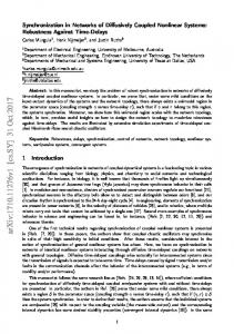
FIG. 1: (Color online) Ratio of interspike intervals hT1 i/hT2 i of the two subsystems in dependence on the coupling strength C and noise intensity D1 . No control is applied to the system. The dots mark the parameter choice for different synchronization regimes used in the following. Other parameters as in Fig. 2.

in Fig. 1 how the frequency synchronization changes in dependence on the coupling strength and noise intensity. For a small value of D1 and large coupling strength, the two subsystems display synchronized behavior, hT1 i/hT2 i ≈ 1. On average, they show the same number of spikes indicated by bright (yellow) color. Since we are interested in the effects of a control force on the synchronization, in the following, we consider three different cases: moderately, weakly, and strongly synchronized systems given by the specific choices of the coupling strength and noise intensity in the first subsystem (C = 0.2, D1 = 0.6), (C = 0.1, D1 = 0.6), and (C = 0.2, D1 = 0.15), respectively. These different cases of stochastic synchronization are marked as black dots in Fig. 1. Strong synchronization can be found for small noise intensity D1 and large C, e.g., D1 = 0.15 and C = 0.2. Moderate synchronization is given for a choice of D1 = 0.6 and C = 0.2, and weak synchronization can be realized by D1 = 0.6 and C = 0.1. In terms of the time series, the three configurations of moderate, weak, and strong synchronization are displayed in Fig. 2 as panels (a), (b), and (c), respectively. In all panels, the black, grey (red), and lightgrey (green) curves refer to the global xΣ -variable, the x2 -, and x1 variable, respectively, where xΣ is given by xΣ = x1 + x2 . Moderately synchronized systems perform mostly synchronized spiking. However, there are certain events where only one system shows an oscillation (see panel (a) of Fig. 2). In the case of weak synchronization, the spikes of the two subsystems coincide less as can be seen from the time series of the summarized signal xΣ in panel (b) of Fig. 2. For strongly synchronized subsystems (see panel (c) of Fig. 2), the time series of the x1 - and x2 variable exhibit spiking at the same time.

0

20

40

60

80

100

(c)

(b)

(a)

x1, x2, xΣ x1, x2, xΣ x1, x2, xΣ

(c)

(b)

(a)

x1, x2, xΣ x1, x2, xΣ x1, x2, xΣ

3

9000

9020

9040

9060

9080

9100

t

t

FIG. 2: (Color online) Time series of the coupled FitzHughNagumo system in the absence of control. Panels (a), (b), and (c) correspond to moderately (C = 0.2, D1 = 0.6), weakly (C = 0.1, D1 = 0.6), and strongly (C = 0.2, D1 = 0.15) synchronized systems, respectively. In all panels, the black, grey (red), and lightgrey (green) curves refer to the summarized variable xΣ = x1 + x2 , the x2 -, and the x1 -variable, respectively. Other parameters: a = 1.05, ǫ1 = 0.005, ǫ2 = 0.1, and D2 = 0.09.

FIG. 3: (Color online) Time series of the coupled FitzHughNagumo system for moderate synchronization. Panel (a) corresponds to no control. In panels (b) and (c), time-delayed feedback is applied to the system with different memory parameters R = 0 and R = 0.9, respectively. Other control parameters are fixed at τ = 1 and K = 1.5. Grayscale (color coding) and other parameters as in Fig. 2.

2.2.

Time series and control

Equation (1a) already includes the time-delayed feedback scheme, whose parameters are the feedback gain K, the time delay τ , and the memory parameter R. The special case of R = 0, also known as Pyragas control [Pyragas, 1992], was already investigated by [Hauschildt et al., 2006]. Therefore, in the present work, we discuss an extension to a different feedback stimulation involving multiple delays. In this extended form, the method generates a control force from the differences of the states of the system that are one time unit τ apart. The memory parameter R ∈ (−1, 1) can be understood as a weight of states that are further in the past. For vanishing memory parameter R = 0, only one delayed state enters the generation of the control force. We consider the case where the control force is applied to the first system only and in the inhibitor variable. Note that one could also realize a feedback scheme that is applied to both subsystems and study effects of different values of the control parameters for each subsystem, but these investigations are out of the scope of this work. Here we put special emphasis on the effects due to changes in the memory parameter. Figure 3 depicts different time series for moderate synchronization (C= 0.2, D1 = 0.6) in the absence of con-

trol (panel(a)) compared to the cases when time-delayed is applied to the system (panels (b) and (c) for memory parameters of R = 0 and R = 0.9). The time delay and feedback gain are chosen as τ = 1 and K = 1.5. In all panels, the black, grey (red), and lightgrey (green) curves correspond to the summarized global signal xΣ , the x2 -, and the x1 -variable, respectively. One can see that the time-delayed feedback enhances the synchronization, i.e., events at which only one system oscillates are less frequent. In this sense the choice of R = 0 is more efficient compared to larger memory parameters.

3.

RATIO OF AVERAGE INTERSPIKE INTERVALS

As first measure to quantify changes in the synchronization due to the control force, in this section, we consider the ratio of average interspike intervals. In the presence of a control force, i.e., K 6= 0, the cooperativity can be influenced by the control parameters. Varying the feedback gain K, the time delay τ , and the memory parameter R, the average interspike interval can be altered. The case of R = 0 was discussed in Ref. [Hauschildt et al., 2006]. For fixed feedback gain K = 1.5 and two different values of R (R = 0 and R = 0.9), Fig. 4 depicts the average interspike intervals of the subsystems, shown as

5

0.8

4

0.75

3 0

2

4

τ

6

8

0.7 10

4

0.65

3

0.6

2 6

0.55 0.75 0.7

5

0.65 4 3 0

0.6 2

4

τ

6

8

0.55 10

1

8 0.96

6

0.92

4 10

1

8 0.96

6 4 0

2

4

τ

6

8

/

,

0.85

0.7

/

0.7

3 6

5

(c) 10 ,

0.75

0.75

/

4

6

,

0.8

/

5

/

0.85

,

(b)

6

,

,

(a)

/

4

0.92 10

FIG. 4: (Color online) Interspike intervals in dependence on the time delay τ . The green dots correspond to the ratio of the interspike intervals hT1 i/hT2 i of the two subsystems, which are also depicted by solid (black) and dashed (red) curves for hT1 i and hT2 i, respectively. Panels (a), (b), and (c) correspond to the case of moderate, weak, and strong synchronization, respectively. The control parameters are chosen as K = 1.5 and the memory parameter corresponds to R = 0 and 0.9 in the top and bottom panels, respectively. Other parameters as in Fig. 2.

solid (black) and dashed (red) curves for hT1 i and hT2 i, and their ratio (as dotted (green) curve) for the case of moderately, weakly, and strongly synchronized systems, respectively, in dependence on the time delay τ . The left, middle, and right panels correspond to the case of moderate, weak, and strong synchronization, respectively. In all cases, tuning of the time delay leads to either enhanced and deteriorated synchronization for R = 0. If more information of past states (R 6= 0) is included, however, the variation of the ratio hT1 i/hT2 i is less sensitive to the specific choice of τ . The bottom panels of Fig. 4 do not show large deviations for the ratio of average interspike intervals. Therefore, a larger memory parameter renders the control method more robust. One can also consider two-dimensional projections of the control parameter space spanned by K, τ , and R. Parameterized by the feedback gain and time delay, Fig. 5 displays the ratio of hT1 i and hT2 i for moderate, weak, strong synchronization, respectively. The four panels in each figure correspond to a memory parameter of R = 0, 0.35, 0.7, and 0.9. Note that Fig. 4 can be understood as horizontal cuts for K = 1.5 in the respective diagram of Fig. 5. As also shown in the one-dimensional projections (see Fig. 4), an increase of the memory parameter R at fixed K yields smaller changes of the ratio hT1 i/hT2 i. Independent on the feedback gain K, the desynchronized darker region in Fig. 5 at a time delay τ ≈ 3 is much less pronounced. For R = 0.9, the ratio of average interspike intervals is constant in a wide range of the whole control domain, which reflects the robustness of this extended feedback method.

4.

POWER SPECTRUM

The two uncontrolled neural populations have different timescales, i.e., ǫ1 6= ǫ2 , and therefore, oscillate at different frequencies. We have shown in the last section

that the mean frequencies of the subsystems measured by the average interspike intervals match for certain control parameters. In order to gain a better understanding of the shift in the timescales in the subsystem in the presence of control, we investigate the power spectrum in this section, where we focus on the role of the memory parameter. At first, we consider the case when no control is applied to the system, i.e., K = 0. The result can be seen in Fig. 6 where the solid (red) and dashed (blue) curves correspond to the power spectrum, of the x1 - and x2 -variable, respectively. The left, middle, and right panel refer to the case of moderate, weak, and strong synchronization, respectively. This change of frequency synchronization is reached by choosing different coupling strengths C and noise intensities D1 . In the case of moderate synchronization (C = 0.2, D1 = 0.6) the peaks of the power spectrum partly overlap. Weak synchronization (C = 0.1, D1 = 0.6) shows a smaller overlap, whereas for strong synchronization (C = 0.2, D1 = 0.15) the spectra almost coincide. Next, we apply extended time-delayed feedback to the system. Figures 7, 8, and 9 show the power spectrum of the summarized signal xΣ = x1 + x2 for the three above mentioned cases of synchronization in dependence on the time delay τ . In all figures, panels (a), (b), and (c) correspond to a memory parameter of R = 0, R = 0.5, and R = 0.9, respectively. The feedback gain is fixed at K = 1.5. It can be seen that, depending on the choice of τ , the main frequency component is shifted. Thus, the control scheme is able to support different timescales. Note that, for instance in the case of moderate synchronization (Fig. 7), the control force enhances the frequency corresponding to the dynamics of the x1 - or x2 -variable. Compare the bright (yellow) areas in Fig. 7 to the middle panel of the uncontrolled case in Fig. 6. A time delay of τ ≈ 3 favors a frequency of f ≈ 0.4, i.e., the main frequency of x1 , and τ ≈ 5 enhances components of f ≈ 0.2,

5 2 R=0

2

0.9

R=0.35

R=0

K

0.5

0 2

0.6 0.9

0 2

R=0.9

τ

0.55 R=0.7

0.8 K

0.75

1 0.5

2

4

6

8

10 0

2

4

τ

6

8

R=0.9

1.0 0.95

1

0.9

0.5 0.55

0.6 0

0.85 R=0.7

1.5

0.65

0.7

0.5

0.9

0 2

R=0.9

1.5

1

0.95

1 0.5

K

R=0.7

τ

1.0

0.65

0.7

1.5

0.75

1

R=0.35

1.5 K

0.8

1

K

R=0.35

1.5

0.5

K

2 R=0

1.5

10

0

2

4

τ

6

8

10 0

2

4

τ

6

8

0.85

10

0

2

τ

4

6

8

10 0

2

τ

4

6

8

10

τ

FIG. 5: (Color online) Ratio of interspike intervals hT1 i/hT2 i in dependence on the feedback gain K and the time delay τ for moderate (C = 0.2, D1 = 0.6), weak (C = 0.1, D1 = 0.6), and strong (C = 0.2, D1 = 0.15) synchronization in the left, middle, and right panel, respectively. The memory parameter are fixed ar R = 0, 0.35, 0.7, and 0.9 in the four subfigures of all three panels. Other parameters as in Fig. 2.

0.02 D1=0.6, C=0.2

D1=0.6, C=0.1

S(f)

S(f)

S(f)

0.01

D1=0.15, C=0.2

0.03

0.02

0.02

0.01 0.01

0

0 0

0.2

0.4

0.6

0.8

1

0 0

0.2

f

0.4

0.6 f

0.8

1

0

0.2

0.4

0.6

0.8

1

f

FIG. 6: (Color online) Power spectrum of the two subsystems in the absence of control. The left, middle, and right panels correspond to the case of moderate, weak, and strong synchronization, respectively. The solid (red) and dashed (blue) curves refer to the x1 - and x2 -variable, respectively. Other parameters as in Fig. 2.

which corresponds to the dynamics of x2 . For larger memory parameters R, this effect is less pronounced. The power spectra of the controlled system display reduced sensitivity on the specific choice of the time delay. The main peak of the spectrum is stronger localized at the frequency of the second subsystem, but the value of the power spectrum at this main frequency is much lower. Figure 10 shows the power spectrum of the global summarized signal xΣ for the three different case of synchronization and fixed time delay τ = 5. In all panels, the solid (black), dashed (red), and and dotted (green) curves correspond to a memory parameter of R = 0, 0.5, and 0.9, respectively. The feedback gain is fixed at K = 1.5. Panels (a), (b), and (c) of Fig. 10 can be seen as horizontal cuts (at τ = 5) of Figs. 7, 8, and 9, respectively. Opposed to the uncontrolled case (see Fig. 6), the power spectra exhibit a series of distinct peaks that are located at the harmonics of the main frequency f ≈ 0.2. They are due to the control force which enhances not only the main frequency, but also frequency components of the higher harmonics. For increasing memory parame-

ter R, the background becomes broader. We stress that a similar effect was found in the context of extended timedelayed feedback applied to the noise-induced oscillations in the Van-der-Pol system [Pomplun et al., 2007] and in a reaction-diffusion system [Majer & Sch¨ oll, 2009], where, in addition, the peaks become sharper.

5.

INTERSPIKE INTERVAL DISTRIBUTION

In the previous Section, we have discussed the modulation of timescales due to time-delayed feedback. To obtain further information about the timescales present in the coupled system, we investigate the probability distribution of the interspike intervals in the following, where we restrict our investigation to the analysis of the summarized signal xΣ = x1 + x2 . Figures 11, 12, and 13 depict the dependence of the distributions of the interspike interval TΣ for moderately (C = 0.2, D1 = 0.6), weakly (C = 0.1, D1 = 0.6), and strongly synchronized (C = 0.2, D1 = 0.15) subsystems on the time delay, respectively. These are the three cases

6

(a) R=0

(b) R=0.5

(c) R=0.9

10

0.12

8 0.08

τ

6 4

0.04

2 0

0 0

0.2

0.4

0.6

0.8 0

0.2

f

0.4

0.6

0.8 0

0.2

f

0.4

0.6

0.8

f

FIG. 7: (Color online) Power spectrum of the summarized signal xΣ = x1 +x2 for moderate synchronization (C = 0.2, D1 = 0.6) in dependence on the time delay τ . Panels (a), (b), and (c) correspond to a memory parameter of R = 0, R = 0.5, and R = 0.9, respectively. The feedback strength is fixed at K = 1.5. Other parameters as in Fig. 2.

(a) R=0

(b) R=0.5

(c) R=0.9

10

0.09

8 0.06

τ

6 4

0.03

2 0

0 0

0.2

0.4

0.6

0.8 0

0.2

f

0.4

0.6

0.8 0

f

0.2

0.4

0.6

0.8

f

FIG. 8: (Color online) Power spectrum of the summarized signal xΣ = x1 + x2 for weak synchronization (C = 0.1, D1 = 0.6) in dependence on the time delay τ . Panels (a), (b), and (c) correspond to a memory parameter of R = 0, R = 0.5, and R = 0.9, respectively. Other parameters as in Fig. 7.

marked in Fig. 1. The corresponding power spectra are shown in Figs. 7, 8, and 9. Panels(a), (b), and (c) in each figure refer to a memory parameter of R = 0, 0.5, and 0.9, respectively. Note that all three figures 11, 12, and 13 display the same greyscale (color code). For increasing memory parameter R, the distribution exhibits a weaker dependence on the time delay τ . This can be seen, for instance, in panels (c) of Figs. 11 and 12. For smaller R values, another effect becomes apparent. There are a minima in the distribution for interspike intervals slightly larger than τ , indicated by black stripes in the (TΣ , τ ) plane. These minima are located below the line TΣ = τ (white line in Fig. 11(a)). A similar, but less pronounced effect can be observed if the interspike intervals match integer multiples of the time delay as shown by the grey line for TΣ = 2τ in the same panel. We stress that for strongly synchronized subsystems this structuring of the interspike interval distribution becomes more visible as displayed in Fig. 13. The probability distribution becomes multimodal with peaks

centered near TΣ = nτ, n = 1, 2, . . . . To summarize this Section, the introduction of a large memory parameter renders the control method more robust against the specific choice of the time delay as is depicted in Fig. 14 for R = 0.99. However, for small memory parameters, there is a competing effect which structures the distribution in the sense that interspike intervals slightly larger than the time delay of the feedback are suppressed.

6.

PHASE SYNCHRONIZATION

The measures for cooperative dynamics considered so far are insensitive to phase relations. A measure of phase synchronization can be obtained by introducing phase variables for each subsystems, and monitoring their difference. For definition of such a phase variable, one can gener-

7

(a) R=0

(b) R=0.5

(c) R=0.9

10

0.18

8 0.12

τ

6 4

0.06

2 0

0 0

0.2

0.4

0.6

0.8 0

0.2

0.4

f

0.6

0.8 0

0.2

0.4

f

0.6

0.8

f

FIG. 9: (Color online) Power spectrum of the summarized signal xΣ = x1 + x2 for strong synchronization (C = 0.2, D1 = 0.15) in dependence on the time delay τ . Panels (a), (b), and (c) correspond to a memory parameter of R = 0, R = 0.5, and R = 0.9, respectively. Other parameters as in Fig. 7. 0.12

0.16

0.08

0.09

0.12

0.06

0.03

0 0 (a)

S(f)

S(f)

S(f)

0.06

0.04

0.04

0.02

0.2

0.6

0.4

0.8

f

0 0

1

0.08

0.2

0.6

0.4 f

(b)

0.8

0

1

(c)

0.2

0.6

0.4

0.8

f

FIG. 10: (Color online) Power spectrum of the summarized signal xΣ = x1 + x2 for a fixed time delay of τ = 5. Panels (a), (b), and (c) correspond the case of moderate (C = 0.2, D1 = 0.6), weak (C = 0.1, D1 = 0.6), and strong (C = 0.2, D1 = 0.15) synchronization. The solid (black), dashed (red), and dotted (green) curves refer to a memory parameter of R = 0, 0.5, and 0.9, respectively. Other parameters as in Fig. 7.

ate a phase from the time series of spikes: ϕ(t) = 2π

t − ti−1 + 2π(i − 1), ti − ti−1

(4)

where ti denotes the time of the i-th spike. With this definition the phase increases by a value of 2π for each spike [Hauschildt, 2005; Hauschildt et al., 2006; Pikovsky et al., 1996, 2001]. The phase difference ∆ϕ between two subsystems can be defined for general n : m synchronization as follows ∆ϕn,m (t) = |ϕ1 (t) −

m ϕ2 (t)|, n

(5)

where ϕ1 (t) and ϕ2 (t) denote the phases of the respective subunits. In this work, we consider only 1 : 1synchronization. In Refs. [Hauschildt et al., 2006; Rosenblum et al., 2001], a measure for the phase synchronization is considered: the so-called synchronization index γ. This quantity is also defined using the phase difference ∆ϕ: p γ = hcos ∆ϕ(t)i2 + hsin ∆ϕ(t)i2 . (6)

It varies between 0 (no synchronization) and 1 (perfect synchronization). If the two subsystems are already strongly synchronized, it is helpful to consider the time intervals during which the phase difference stays in a 2π-phase range [Lai et al., 2006; Park & Lai, 2005; Park et al., 2007]. In these synchronization intervals, the subsystems exhibit the same number of spikes. In the case of strong synchronization, the synchronization index γ shows only small changes near its maximum value, whereas the time interval of constant phase difference can vary significantly. A measure of the amount of synchronization is given by the average length δ of the synchronization intervals. The stronger sensitivity, as compared to γ, can be seen in Fig. 16, which depicts the average phase synchronization interval δ as black dots (solid curve) and the synchronization index γ as red squares (dashed line) for varying time delay τ . The other control parameters are chosen as R = 0 and K = 1.5. The scale is chosen such that the points for τ = 0 and τ = 10 coincide. Note that the average phase synchronization interval δ shows a stronger increase than the synchronization index γ. Since the av-

8

(a) R=0

(b) R=0.5

(c) R=0.9

10

0.12

8

0.09

6 τ

0.06

4 2

0.03

0

0 2

4

6 TΣ

8

10 2

4

6 TΣ

8

10 2

4

6 TΣ

8

10

FIG. 11: (Color online) Interspike interval (TΣ ) distribution of the summarized signal xΣ = x1 +x2 for moderate synchronization (C = 0.2, D1 = 0.6) in dependence on the time delay τ . The greyscale (color coding) denotes the probability of finding a certain interspike interval TΣ . Panels (a), (b), and (c) correspond to a memory parameter of R = 0, R = 0.5, and R = 0.9, respectively. The white and grey dotted lines in panel (a) at τ = TΣ and τ = TΣ /2, respectively, are guides to the eye. Other parameters as in Fig. 7.

(a) R=0

(b) R=0.5

(c) R=0.9

10

0.12

8

0.09

6 τ

0.06

4 2

0.03

0

0 2

4

6 TΣ

8

10 2

4

6 TΣ

8

10 2

4

6 TΣ

8

10

FIG. 12: (Color online) Interspike interval (TΣ ) distribution of the summarized signal xΣ = x1 + x2 for weak synchronization (C = 0.1, D1 = 0.6) in dependence on the time delay τ . The greyscale (color coding) denotes the probability of finding a certain interspike interval TΣ . Panels (a), (b), and (c) correspond to a memory parameter of R = 0, R = 0.5, and R = 0.9, respectively. Other parameters as in Fig. 7.

erage phase synchronization interval δ is more sensitive to the control parameters K, τ , and R than the synchronization index γ, we restrict our investigations to the discussion of δ. Figure 15 displays the time evolution of the phase difference ∆ϕ, when no control is applied to the system. The solid (black), dashed (red), and dash-dotted (green) curves correspond to the case of moderate (C = 0.2, D1 = 0.6), weak (C = 0.1, D1 = 0.6), and strong (C = 0.2, D1 = 0.15) synchronization, respectively. The inset depicts an enlargement for moderate synchronization. From this inset, one can clearly see the plateaus in between phase jumps of 2π. At these jumps, only one subsystem shows a spike whereas the other one remains subthreshold. For better synchronization, the slope of ∆ϕ becomes flatter. In the case of strong synchronization, for instance, ∆ϕ shows only a few phase jumps and remains in a 2π-range for large time intervals. The quan-

tity δ measures the average lengths of these intervals. Figure 17 shows effects of extended time-delayed feedback in the average phase synchronization interval δ for varying time delay τ . The feedback gain K is fixed at K = 1.5. Panels (a), (b), and (c) display the case of moderately, weakly, and strongly synchronized subsystems, respectively. In all panels, the solid (black), dashed (red), and dotted (green) curves refer to a memory parameter of R = 0, R = 0.5, and R = 0.9, respectively. The insets in panels (a) and (b) are enlargements for small time delays and the inset in panel (c) display large values of δ. In general, time-delayed feedback enlarges the average phase synchronization interval δ. Especially for small time delays, e.g., τ = 0.7 for R = 0, δ becomes substantially larger. For R = 0, a modulation of δ can be seen for small delays, see insets in all panels of Fig. 17. These deviations are less pronounced for increasing R. Only

9

(a) R=0

(b) R=0.5

(c) R=0.9

10

0.12

8

0.09

6 τ

0.06

4 2

0.03

0

0 2

4

6 TΣ

8

10 2

4

6 TΣ

8

10 2

4

6 TΣ

8

10

FIG. 13: (Color online) Interspike interval (TΣ ) distribution of the summarized signal xΣ = x1 + x2 for strong synchronization (C = 0.2, D1 = 0.15) in dependence on the time delay τ . The greyscale (color coding) denotes the probability of finding a certain interspike interval TΣ . Panels (a), (b), and (c) correspond to a memory parameter of R = 0, R = 0.5, and R = 0.9, respectively. Other parameters as in Fig. 7.

(a) moderate

(b) weak

(c) strong

10

0.09

8 0.06

τ

6 4

0.03

2 0

0 2

4

6 TΣ

8

10 2

4

6 TΣ

8

10 2

4

6 TΣ

8

10

FIG. 14: (Color online) Interspike interval (TΣ ) distribution of the summarized signal xΣ = x1 + x2 in dependence on the time delay τ for a memory parameter R = 0.99 for moderate (C = 0.2, D1 = 0.6), weak (C = 0.1, D1 = 0.6), and strong (C = 0.2, D1 = 0.15) synchronization in panels (a), (b), and (c), respectively. The greyscale (color coding) denotes the probability of finding a certain interspike interval TΣ . Other parameters as in Fig. 7.

panel (c), which refers to strong synchronization, shows larger values of δ with increasing memory parameter. The sensitivity of δ, as discussed in Fig. 16, can also be seen in the case of strong synchronization. See panel (c) in Fig. 17. Since the already strong synchronization is further enhanced by the control force, the average phase synchronization interval rises by several orders of magnitude as shown in the inset. For perfect synchronization and simultaneous spiking, δ would be arbitrarily large and merely reflect the integration time.

7.

CONCLUSION

We have investigated the cooperative dynamics of two symmetrically coupled neurons under the effects of local extended time-delayed feedback. We have found that the specific choice of the control parameters, i.e., feedback

gain K, time delay τ , and memory parameter R, alters the cooperativity, which we have discussed in the context of different measures of synchronization: ratio of average interspike intervals and average phase synchronization intervals. If the control force is generated including states further in the past, i.e., for larger memory parameter, the two subsystems exhibit enhanced phase synchronization, if the uncontrolled system is already in the strong synchronization regime. In general, both the frequency and phase synchronization as well as the interspike interval distribution become less sensitive to variations in τ with increasing R. A small memory parameter R leads to a suppression of interspike intervals slightly larger than the time delay. The stability of a synchronous manifold for coupled ordinary differential equations can be investigated by means of a master stability function [Chavez et al., 2005; Pecora & Carroll, 1998]. For delay differential equations involving stochastic input, this formalism is not yet devel-

10 oped. Future investigations should address this to obtain an analytical understanding of the control of synchronization in neural networks by time-delayed feedback.

120

∆ϕ [2π]

240

180

110 100 500

600

700

120

60

0 0

200

600

400

800

1000

t

FIG. 15: (Color online) Phase difference in units of 2π. The solid (black), dashed (red), and dash-dotted (green) curves correspond to the case of moderate (C = 0.2, D1 = 0.6), weak (C = 0.1, D1 = 0.6), and strong (C = 0.2, D1 = 0.15) synchronization, respectively. No control is applied to the system. The inset shows an enlargement for moderate synchronization. Other parameters as in Fig. 2. 35 δ γ

30

1.1 1

25

γ

δ

0.9

20

0.8 0.7

15

Acknowledgments

0.6 10 0

2

4

τ

6

8

0.5 10

FIG. 16: (Color online) Average phase synchronization interval δ (black dots, solid curve) and synchronization index γ (red squares, dashed line) in dependence on the time delay τ for the case of moderately synchronized subsystems and vanishing memory parameter R. Other parameters as in Fig. 15.

This work was supported by DFG in the framework of Sfb 555 (Complex Nonlinear Processes). P. H. acknowledges support of the Deutsche Akademische Austauschdienst (DAAD) and thanks Kazuyuki Aihara and his group for stimulating discussions.

Balanov, A. G., Beato, V., Janson, N. B., Engel, H. & Sch¨ oll, E. [2006] “Delayed feedback control of noiseinduced patterns in excitable media,” Phys. Rev. E 74, 016214. Balanov, A. G., Janson, N. B. & Sch¨ oll, E. [2004] “Control of noise-induced oscillations by delayed feedback,” Physica D 199, 1. Chavez, M., Hwang, D. U., Amann, A., Hentschel, H. G. E. & Boccaletti, S. [2005] “Synchronization is Enhanced in Weighted Complex Networks,” Phys. Rev. Lett. 94, 218701.

Dahms, T., H¨ ovel, P. & Sch¨ oll, E. [2007] “Control of unstable steady states by extended time-delayed feedback,” Phys. Rev. E 76(5), 056201. Dahms, T., H¨ ovel, P. & Sch¨ oll, E. [2008] “Stabilizing continuous-wave output in semiconductor lasers by time-delayed feedback,” Phys. Rev. E Submitted. Flunkert, V. & Sch¨ oll, E. [2007] “Suppressing noise-induced intensity pulsations in semiconductor lasers by means of time-delayed feedback,” Phys. Rev. E 76, 066202. Gassel, M., Glatt, E. & Kaiser, F. [2007] “Time-delayed feed-

11 35

16

R = 0.5 R=0 R = 0.9

30

12

25

5.0 ·10 2000

30 20 10 0 0

10 5 2

8

16

6

12

4

8

4

τ

1 6

1.5 8

2

0 0

10

0 0

2

4

6

8

10

1000 500

0 0 2

R=0 R = 0.5 R = 0.9

4

1500

4

2

0.5

5

δ

δ

δ 15

0 0

1.0 ·10 2500

10

20

(a)

3000

R=0 R = 0.5 R = 0.9

14

0.5 4

(b)

τ

1 6

1.5 8

2

0 0

10 (c)

2

4

τ

6

8

10

FIG. 17: (Color online) Average phase synchronization interval δ in dependence on the time delay τ . The solid (black), dashed (red), and dotted (green) curves correspond to a memory parameter of R = 0, R = 0.5, and R = 0.9, respectively. The panels (a), (b), and (c) refer to the case of moderate, weak, and strong synchronization, respectively. The insets in panels (a) and (b) show an enlargement for small τ . The inset in panel (c) displays large δ. Other parameters as in Fig. 15.

back in a net of neural elements: Transitions from oscillatory to excitable dynamics,” Fluct. Noise Lett. 7(3), L225. Gassel, M., Glatt, E. & Kaiser, F. [2008] “Delaysustained pattern formation in subexcitable media,” Phys. Rev. E 77(6), 066220 (pages 7). Hauschildt, B. [2005] Control of noise-induced multimode oscillations in coupled neural systems Master’s thesis TU Berlin. Hauschildt, B., Janson, N. B., Balanov, A. G. & Sch¨ oll, E. [2006] “Noise-induced cooperative dynamics and its control in coupled neuron models,” Phys. Rev. E 74, 051906. Hizanidis, J., Balanov, A. G., Amann, A. & Sch¨ oll, E. [2006] “Noise-induced front motion: signature of a global bifurcation,” Phys. Rev. Lett. 96, 244104. Hizanidis, J. & Sch¨ oll, E. [2008] “Control of noiseinduced spatiotemporal patterns in superlattices,” phys. stat. sol. (c) 5(1), 207. Janson, N. B., Balanov, A. G. & Sch¨ oll, E. [2004] “Delayed Feedback as a Means of Control of Noise-Induced Motion,” Phys. Rev. Lett. 93, 010601. Lai, Y. C., Frei, M. G. & Osorio, I. [2006] “Detecting and characterizing phase synchronization in nonstationary dynamical systems,” Phys. Rev. E 73(2), 26214. Majer, N. & Sch¨ oll, E. [2009] “Resonant control of stochastic spatio-temporal dynamics in a tunnel diode by multiple time delayed feedback,” Phys. Rev. E . Park, K. & Lai, Y. C. [2005] “Characterization of stochastic resonance,” Europhys. Lett 70(4), 432. Park, K., Lai, Y. C. & Krishnamoorthy, S. [2007] “Noise sensitivity of phase-synchronization time in stochastic resonance: Theory and experiment,” Phys. Rev. E 75(4), 46205. Pecora, L. M. & Carroll, T. L. [1998] “Master Stability Functions for Synchronized Coupled Systems,” Phys. Rev. Lett. 80(10), 2109. Pikovsky, A., Rosenblum, M. G. & Kurths, J. [1996] “Synchronisation in a population of globally coupled chaotic oscillators,” Europhys. Lett. 34, 165. Pikovsky, A., Rosenblum, M. G. & Kurths, J. [2001] Synchronization, A Universal Concept in Nonlinear Sciences (Cambridge University Press, Cambridge). Pomplun, J., Amann, A. & Sch¨ oll, E. [2005] “Mean field

approximation of time-delayed feedback control of noise-induced oscillations in the Van der Pol system,” Europhys. Lett. 71, 366. Pomplun, J., Balanov, A. G. & Sch¨ oll, E. [2007] “Longterm correlations in stochastic systems with extended time-delayed feedback,” Phys. Rev. E 75, 040101(R). Popovych, O. V., Hauptmann, C. & Tass, P. A. [2005] “Effective Desynchronization by Nonlinear Delayed Feedback,” Phys. Rev. Lett. 94, 164102. Popovych, O. V., Hauptmann, C. & Tass, P. A. [2006] “Control of neuronal synchrony by nonlinear delayed feedback,” Biol. Cybern. 95(1), 69. Pototsky, A. & Janson, N. B. [2007] “Correlation theory of delayed feedback in stochastic systems below Andronov-Hopf bifurcation,” Phys. Rev. E 76, 056208. Pototsky, A. & Janson, N. B. [2008] “Excitable systems with noise and delay, with applications to control: Renewal theory approach,” Phys. Rev. E 77(3), 031113 (pages 11). Prager, T., Lerch, H. P., Schimansky-Geier, L. & Sch¨ oll, E. [2007] “Increase of Coherence in Excitable Systems by Delayed Feedback,” J. Phys. A 40, 11045. Pyragas, K. [1992] “Continuous control of chaos by selfcontrolling feedback,” Phys. Lett. A 170, 421. Rosenblum, M., Pikovsky, A., Kurths, J., Sch¨ afer, C. & Tass, P. A. [2001] Phase synchronization: from theory to data analysis (Elsevier Science, Amsterdam) volume 4 of Handbook of Biological Physics chapter 9 pp. 279–321. Rosenblum, M. G. & Pikovsky, A. [2004a] “Controlling Synchronization in an Ensemble of Globally Coupled Oscillators,” Phys. Rev. Lett. 92, 114102. Rosenblum, M. G. & Pikovsky, A. [2004b] “Delayed feedback control of collective synchrony: An approach to suppression of pathological brain rhythms,” Phys. Rev. E 70, 041904. Schiff, S. J., Jerger, K., Duong, D. H., Chang, T., Spano, M. L. & Ditto, W. L. [1994] “Controlling Chaos in the brain,” Nature (London) 370, 615. Schlesner, J., Amann, A., Janson, N. B., Just, W. & Sch¨ oll, E. [2003] “Self-stabilization of high frequency oscillations in semiconductor superlattices by time–delay

12 autosynchronization,” Phys. Rev. E 68, 066208. Sch¨ oll, E., Balanov, A. G., Janson, N. B. & Neiman, A. [2005] “Controlling stochastic oscillations close to a Hopf bifurcation by time-delayed feedback,” Stoch. Dyn. 5, 281. Sch¨ oll, E., Majer, N. & Stegemann, G. [2008] “Extended time delayed feedback control of stochastic dynamics in a resonant tunneling diode,” phys. stat. sol. (c) 5(1), 194. Sch¨ oll, E. & Schuster, H. G. (eds.). [2008] Handbook of Chaos Control (Wiley-VCH, Weinheim) second completely revised and enlarged edition.

Socolar, J. E. S., Sukow, D. W. & Gauthier, D. J. [1994] “Stabilizing unstable periodic orbits in fast dynamical systems,” Phys. Rev. E 50, 3245. Stegemann, G., Balanov, A. G. & Sch¨ oll, E. [2006] “Delayed feedback control of stochastic spatiotemporal dynamics in a resonant tunneling diode,” Phys. Rev. E 73, 016203. Unkelbach, J., Amann, A., Just, W. & Sch¨ oll, E. [2003] “Time–delay autosynchronization of the spatiotemporal dynamics in resonant tunneling diodes,” Phys. Rev. E 68, 026204.