Proceedings of the 2007 American Control Conference Marriott Marquis Hotel at Times Square New York City, USA, July 11-13, 2007
ThC06.5
Control Oriented Modeling of Combustion Phasing for an HCCI Engine Mahdi Shahbakhti and Charles Robert Koch
Abstract— A promising method for reducing emissions and fuel consumption of internal combustion engines is the Homogeneous Charge Compression Ignition (HCCI) engine. Control of ignition timing must be realized before the potential benefits of HCCI combustion can be implemented in production engines. A model suitable for real time implementation is developed and this model is able to predict ignition timing with an average error of less than 2 crank angle degrees. A modified knockintegral model (MKIM), with correlations for gas exchange process and fuel heat release, is used to predict HCCI combustion timing (CA50, crank angle where 50% of the fuel mass is burnt). The MKIM model is parameterized using a thermokinetic simulation model. Experimental data from a single cylinder engine at several HCCI operation conditions and three fuel blends is used to validate the model.
I. I NTRODUCTION In an HCCI engine, premixed air and fuel are compressed until the charge autoignites. This results in homogeneous combustion with fast heat release that can significantly reduce NOx and particulate emissions, while achieving high thermal efficiency. In an HCCI engine the charge composition at intake valve closing is the predominant factor affecting combustion timing. The control of ignition timing is critical in order to make HCCI practical for production engines [1]. Despite the extensive work done on controloriented modeling of HCCI ignition timing, improved models that work with easily measurable inputs and which include variable engine working conditions are still needed. Several model types have been used to simulate the ignition timing of HCCI engines. They differ in the complexity and required input data. These models range from multidimensional CFD models ([2], [3]) and multi-zone models ([4], [5]), to simple control-oriented models [6], [7]. For real-time control, a compromise between the computation time and the accuracy of the model is required. Low-order control oriented models can predict HCCI ignition timing with a reasonable accuracy while having short computational time [8]. Several approaches to control oriented modeling of HCCI combustion have been investigated. In the simplest approach, HCCI ignition timing is measured as a function of engine variables that affect HCCI combustion [9] but this requires a large number of experiments. A temperature threshold to find the start of combustion [10] is another simple modeling method but may fail to capture combustion phasing at different operating conditions. The This work was supported in part by the Natural Sciences and Engineering Research Council of Canada Grant number 249553-02 and by AUTO21 Network of Centres of Excellence, under Research Grant number D05-DEC. M. Shahbakhti and C.R. Koch are with the Department of Mechanical Engineering, University of Alberta (e-mail:
[email protected];
[email protected]).
1-4244-0989-6/07/$25.00 ©2007 IEEE.
Shell model [11] is used in [6] to predict HCCI ignition timing with an accurate estimation of the HCCI ignition timing for temperature and engine speed variations, but with less accurate results when changing the load. In [6], [8], [12], models based on Arrhenius-type reaction rate [13] are used. This model type is accurate, but requires instantaneous fuel and oxygen concentrations and in-cylinder gas temperature which are impractical to measure. To remove the need for incylinder composition data, some researchers [14], [15] omit the mixture composition term from the Arrhenius reaction rate and assume that the composition term in Arrhenius reaction rate is of secondary importance compared to other terms. Their results seem accurate in the studied HCCI range, but still need to be validated over a wide range of HCCI operation. The knock-integral model [16] is another category of control-oriented modeling of HCCI combustion timing. This model is based on an exponential correlation which includes the elements of in-cylinder gas pressure and temperature to predict the auto-ignition of a homogeneous mixture [17], [18], [19]. Although this model produces accurate results, again there are some variables that are difficult and expensive to measure, limiting the real-time control application of this model. To improve existing models, another category of models has been developed [19], [20], [21] and [22]. The model proposed in this paper is designed to be a control-oriented model which also works for different engine conditions including variable load, air temperature, engine speed, air fuel ratio (AFR), and EGR (Exhaust Gas Recirculated). Instantaneous in-cylinder gas temperature, pressure and concentrations of fuel and oxygen are not required, instead measured AFR, EGR and intake gas temperature and pressure are required. This model extends our previous work [22] because the inputs are easier to measure (the intake temperature and pressure) and CA50 is predicted. In this paper, section II explains the model developed to predict HCCI combustion timing. Section III shows the methodology used to parameterize the model and section IV explains the experimental setup and conditions of the HCCI test points. Finally, the proposed model is experimentally validated and conclusions are reached. II. M ODEL D ESCRIPTION A. IVC temperature & pressure correlation HCCI combustion is mainly affected by the properties of air fuel mixture at Intake Valve Closing (IVC). To predict the start of combustion (SOC) our offline HCCI simulation requires temperature and pressure of the air fuel mixture at IVC. Since temperature and pressure of the air fuel mixture
3694
ThC06.5
Pivc
N 0.038 Φ0.020 Pman = 0.022 Tman
(1)
where, N is presented in rpm and Pman in kiloPascals (kPa) and Tman in Celsius (C). Using the correlation (1) over available experimental data, the average error and error standard deviation are 1.33 kPa and 0.97 kPa respectively and the maximum relative error is less than 4%. Since it is difficult to experimentally measure the mixture temperature at IVC, the values of Tivc , are obtained from Thermo-Kinetic Model simulation (TKM1 ) which is run for all the experimental HCCI points used in this study. Simulated Tivc values that match experimental SOC are chosen as the correct Tivc . By plotting the change of Tivc with respect to Tman , it was noticed that after a specific intake temperature (i.e. Tman = 110o C), Tivc decreases with an increase in Tman , while the reverse trend is seen for the cases with Tman lower than 110o C. This comes from a change in the direction of heat transfer between the incylinder mixture and cylinder walls, where a constant wall temperature is assumed in the TKM for all the available HCCI experiments. The following correlation was found based on the available experimental data: Tivc = (a . Tman + b)
Φc . N d e (1 + EGR)
(2)
where a, b, c, d, and e are the parameters of the correlation that should be determined and Φ represents equivalence ratio of the air-fuel mixture. The correlation suggests a linear relation between gas temperature at IVC and the intake manifold temperature. The sign of a changes from positive to negative from the cases with Tman < 1100 C to the cases with Tman ≥ 1100 C. This implies to the change of heat transfer direction after a certain thermal condition. The correlation also suggests that Tivc is increased with an increase in engine speed. This can be caused by a combination effects of pressure rise in cylinder gas and the less available time for heat transfer. Furthermore, for the zone of Tman < 1100 C, Tivc is decreases with an increase in EGR, while it increases with an increase in equivalence ratio. This trend is reversed when Tman ≥ 1100 C. This is because of the influence of EGR and Φ on the heat transfer, while the direction of heat transfer is controlled by the temperature difference between the in-cylinder gas temperature and cylinder wall temperature. Increasing EGR 1 The
details of the TKM is explained later in section III.
B. SOC Model The original Knock Integral Model (KIM) for predicting SOC of HCCI engine is introduced and then modified in this section. 1) Knock Integral Model (KIM): Kinetics of HCCI combustion are very similar to the chemical kinetics of knock in SI (Spark Ignition) engines [15]. Knock in SI engines has been investigated for decades [16], [23]. Livengood and Wu [16] developed a correlation to predict the autoignition of a homogeneous mixture, it was later termed the Knock-Integral Model (KIM) [24]. Livengood and Wu proposed that there is a functional relationship between the concentration ratio, (x)/(x)c , of the significant species in the reaction and the relative time, t/τ . The critical concentration ratio, (x)c , is the concentration of the species at the end of the reaction being studied. Using the crank angle instead of time, the ignition correlation of Livengood and Wu becomes: Z θ=θe Z θ=θe 1 1 (x) = dθ = dθ = 1.0 (3) (b/T )pn (x)c ωτ Aωe θo =0 θo =0 where τ is the ignition delay, T is the mixture temperature as a function of time, p is the mixture pressure as a function of time. A, b, and n are empirical constants which are determined for each engine. θe represents the crank angle that autoignition or knock occurs and θo is the initial crank angle that the integration begins. The engine speed (ω) is represented in rpm, the pressure in kiloPascals (kPa), and the temperature in Kelvin (K). The value of θo is selected to be the crank angle of IVC timing where no appreciable reaction has begun (θo = θIV C ). The value of the expression being integrated increases as the point of autoignition is approached as shown in Figure 1.
0.5
n
The following correlation is found to fit well on the available experimental data:
leads to an increase in the specific heat capacity of the mixture which reduces the rate of heat transfer. Using the correlation (2) for the available experimental data, the maximum average error and maximum error standard deviation are 3.1o C and 2.9o C respectively.
1/(ω τ(θ)) = [A ω e b/T * p ] −1
are easily measured in the intake manifold, correlations are used to predict pressure and temperature of the mixture at IVC from the measured values of the intake manifold. Two correlations for Pivc and Tivc are detailed below.
0.4
0.3
0.2
ivc
0.1
0 −140
Fig. 1.
∫θθsoc 1/(ω τ(θ)) dθ= 1.0 Intake valve closing, θivc = −125o
−120
−100
−80 −60 −40 Crank Angle [aTDC]
θ
soc
−20
0
Graphical integration of 1/(ωτ ) from the IVC to the SOC.
In this study, experimental SOC is defined as being the point at which the third derivative of the pressure trace with
3695
ThC06.5 respect to the crank angle (θ) in CAD (Crank Angle Degree) exceeds a heuristically determined limit [25]: ¯ kPa d3 P ¯¯ = 0.0125 (4) ¯ 3 dθ ign CAD3 2) Modified Knock-Integral Model (MKIM): Although the KIM can predict HCCI ignition, it is impractical for a real engine operation. Engine conditions, such as temperature, pressure and mass fraction burned must be continuously available during compression. In simulations this is possible but on an engine it is not practical. Furthermore, the KIM is restricted to engine operation at a constant AFR without EGR. To adapt KIM to an HCCI engine which has varying AFR rates and EGR these factors need to be included by the following three modifications: • To avoid the requirement of crank angle measurements of temperature and pressure during the engine compression, the temperature and pressure rise in the cylinder is assumed to occur as a polytropic process [14]. This assumption neglects any pre-ignition heating resulting from reactions that occur before the SOC. • The SOC changes when the concentrations of the fuel and oxygen are varied [1], [26]. A crank angle measurement of these concentrations is available in the TKM simulation and can be used in a modified KIM to account for the AFR changes but this information is not available in the real engine. The concentrations of the fuel and oxygen are indicative of the equivalence ratio [6], [10]. The equivalence ratio is a good indication of both the amount of fuel and air concentrations in the engine charge and it can be easily measured on an operating engine using a broadband oxygen sensor. Therefore, an equivalence ratio term is added to the KIM to account for the changes in AFR of the mixture. • For some fuels such as iso-octane the amount of EGR seems to affect SOC. To generalize the correlation for these fuels, one term is added to account for the changes in EGR levels. The resulting MKIM is [22]: Z θSOC Φx µ ¶ dθ = 1.0 (5) b(PIV C vcnc )n θIV C Aω exp T nc −1 v IV C
vc (θ) =
c
V (θIV C ) , A = C1 EGR + C2 V (θ)
phasing [27]. CA50 seems to be a robust indication of HCCI combustion timing, since a small error of combustion phasing results in a small error of the phasing in CAD as the slope of energy release is very steep. CA50 is useful for feedback control of HCCI combustion [27]. A modified Wiebe function to predict fuel Mass Fraction Burned (MFB) is used to calculate CA50: ¸n ¶ µ · θ − θs (6) xb (θ) = 1 − exp −a θd θd = CD(1 + EGR)x Φy where, θs and θd are SOC crank angle and combustion duration (here 0.5 is 50%) in CAD respectively. θs , EGR and Φ are the three required inputs. Values of θs come from the MKIM and parameters a, n, CD, x , and y are determined by applying an estimation code on the experimental data. As seen in the correlation, combustion duration varies with a change in Φ and EGR level which is consistent with the observations in [1], [26] and [27]. III. M ODEL S ETUP To parameterize and validate the MKIM model requires three steps that are detailed below. A. Thermokinetic Model Simulations For accurate parameter estimation, the MKIM requires data from the engine at many different working conditions. TKM simulation is used as a virtual engine to provide the required data to parameterize the MKIM. The TKM is a single zone thermo-kinetic model [28] which describes the in-cylinder thermo-kinetic state of an HCCI engine from IVC to exhaust valve opening. The chemical kinetic mechanism, consisting of 58 species and 102 reactions, is used to describe the ignition and combustion of arbitrary blends of a Primary Reference Fuel (PRF) mixture of N-heptane and Iso-octane. The resulting model which couples together the thermodynamic model with the chemical kinetic mechanism was validated with HCCI experimental data from [29]. The model is calibrated for the single-cylinder engine described in Table I. To calibrate the TKM for the new engine, less than 10% of the experimental points, that later will be used to validate the MKIM, are used. The TKM predicts SOC for the single-cylinder engine with a maximum error of 1 CAD over the different conditions.
where, C1 , C2 , b, n, nc , and x are constant parameters. The constant nc represents the average specific heat capacity ratio of all the simulations determined by a numeric best fit. The cylinder volume, V (θ), is calculated at any crank angle from engine geometry. 3) Combustion Phasing (CA50): Combustion duration of an HCCI engine can differ considerably with the same SOC. The crank angle where 50% of fuel mass has burned, denoted here as CA50, is the best indication of HCCI combustion
3696
TABLE I C ONFIGURATIONS OF THE R ICARDO SINGLE - CYLINDER ENGINE Parameters Bore × Stroke [mm] Compression Ratio Displacement [L] Number of Valves IVC [aBDC] EVO [aBDC]
Values 80 × 88.9 10 0.447 4 55◦ −70◦
ThC06.5 TABLE III
The engine speed, initial mixture temperature and pressure, EGR percentage, and equivalence ratio are varied over the ranges outlined in Table II and a TKM simulation is performed. The parameter ranges given in Table II are chosen to represent typical HCCI operation of the Ricardo singlecylinder engine.
E NGINE ’ S OPERATING CONDITIONS FOR HCCI VALIDATION Engine Speed Manifold Temperature EGR(%) Equivalence Ratio Manifold Pressure Fuel Coolant Temperature Oil Temperature
TABLE II PARAMETER VARIATIONS CARRIED OUT USING THE TKM Engine Speed Initial Temperature EGR(%) Equivalence Ratio Initial Pressure Fuel Wall temperature
800, 1000 rpm 80, 85,..., 155, 160 o C 0, 10, 20, 30 0.5, 0.6, 0.7, 0.8 95, 100, 105, 110, 115 kPa PRF0, PRF10, PRF20 390 ◦ K
V. R ESULTS & D ISCUSSION
From the resulting 8160 simulations, complete combustion occurred in 5131 simulations. Since near to TDC firing conditions are of practical interest, late ignited2 TKM simulations are excluded. This results in 4727 TKM simulations which are used to estimate the MKIM parameters. B. Finding the Polytropic Parameter Using the engine parameter variations for the applied PRF fuels, the values of nc can be determined by fitting a best polytropic relation between the temperature or pressure at IVC and SOC of the simulations. The value of nc = 1.32 is chosen using the simulation results of [22]. C. Optimizing the MKIM Parameters The parameters of the MKIM equation (5) are fit to minimize the error of the integration, where the target value is 1.0. The numerical minimization is performed using the built-in Matlab function f minsearch, which uses the Nelder-Mead simplex minimization method [30]. IV. E XPERIMENTAL S ETUP A single cylinder Ricardo Hydra Mark III engine with a Rover K7 head is used to run the HCCI experiments – see Table III. Port fuel injection is used and is timed to ensure closed intake valves. The fresh intake air entering the engine is heated by the electric air heater positioned upstream of the throttle body. Exhaust gases are recirculated (EGR) using an insulated return line from the exhaust to the intake manifold directly after the throttle body. Intake temperature is measured with a K-type thermocouple to include EGR heating effects. The cylinder pressure is measured with a Kistler ThermoCOMP (model 6043A60) piezoelectric pressure sensor that is flush mounted in the cylinder. For each experimental point, pressure traces from 100 consecutive engine cycles are recorded with 0.1 CAD resolution. 2 TKM
800, 1000 rpm 60 - 140 o C 0 - 28.5 0.43 - 0.95 90.5 - 96.3 kPa PRF0, PRF10, PRF20 70 - 80 o C 70 - 80 o C
simulations in which the second stage of HCCI combustion happens at the crank angle higher than 15 degrees after TDC.
Using 4727 TKM simulations, the parameters of the MKIM are determined. The estimation process is done in two stages. In the first stage, parameters b, n, x, and A are determined by applying the estimation code on the all the TKM simulation results. Then, the parameter A is determined for each group of TKM simulations with the same EGR level, keeping the values of b, n, and x constant from the first stage. Figure 2 indicates the predicted SOC for PRF20 TKM simulations with and without the EGR term. As seen in the figure, both average error and error standard deviation are substantially reduced when EGR level is considered in the MKIM. In addition, Figure 2 shows the accuracy of the MKIM predictions deteriorates for late ignitions. This is because the pre-ignition heating by the reactions that occur during the large time span before late ignitions violates the polytropic assumption used in the MKIM. For 709 points in the Figure 2, the average error and error standard deviation are 1.68 CAD and 1.41 CAD respectively. The range of average error and error standard deviation for all TKM simulations are 1.62-2.25 CAD and 1.38-1.79 CAD respectively. Sample values of parameters A, b, n, nc , and x in equation (5) determined for the PRF blends are shown in Figure 2. The order and sign of these parameters are the same for all TKM simulations. By examining these parameters it can be seen that for the three PRF blends the SOC advances by increasing the initial temperature and initial pressure, while it retards with an increase in the engine speed. This trend has been also observed in [6]. Furthermore for all three PRF blends studied, SOC happens sooner when equivalence ratio is increased, while SOC is delayed when EGR level is increased (at constant temperature) similar to [1]. The 4727 points, partly shown in Figure 2, cover a substantial range of initial temperature, equivalence ratio, EGR, initial pressure, and engine speed extending previous work [14], [6], [10], [19], [21] on control-oriented modeling of HCCI ignition timing. However, the model still needs to be cross validated with experimental data which is the subject of the next section. A. Experimental Validation The MKIM has been parameterized by the TKM simulation. The real test of the MKIM model is how well it works with the experimental data from HCCI experiments
3697
ThC06.5 Without EGR Term
15
Ave. Error from Exp. Range = 0.61 CAD
10
Ave. Error = 2.74 CAD
20 Std. Error = 1.92 CAD
5
0 A = 1.4038e−002
−5
b = 1624 n = −0.0306
−10
15
10
n = 1.320 c
5
x = 0.171
−15 −15
−10
15
EGR = 0 EGR = 0.1 EGR = 0.2 EGR = 0.3
−5 0 5 10 Actual Start of Combustion [CADaTDC]
15
With EGR Term
0 0
PRF0
5
10
15
PRF20
PRF10
20
25 30 Case
35
40
45
50
N= 1000 rpm
10 Ave. Error = 1.68 CAD
30 Ave. Error = 1.44 CAD
5 Std. Error = 1.41 CAD
Ave. Error from Exp. Range = 0.02 CAD
25
0 A = 0.0051 * EGR + 0.0133
−5
SOC [Degree aTDC]
Predicted Start of Combustion [CADaTDC]
Predicted Ave. of individual cycles Exp. data range
25 Ave. Error = 1.96 CAD
SOC [Degree aTDC]
Predicted Start of Combustion [CADaTDC]
N= 800 rpm
EGR = 0 EGR = 0.1 EGR = 0.2 EGR = 0.3
b = 1624 n = −3.065e−002
−10
n = 1.320 c
x = 0.171
−15 −15
−10
−5 0 5 10 Actual Start of Combustion [CADaTDC]
15
20
15
10
Fig. 2. Predicted SOC for PRF20 TKM simulations at various engine conditions at 800 rpm using the MKIM. The line represents where the prediction is the same as the actual SOC.
5
described in section IV. In Figure 3 the MKIM predicted SOC values are compared to the corresponding experimental points for three different fuels at different conditions. Since the experimental data consists of 100 measured cycles the range of SOC variation is also shown for each HCCI experiment. Figure 3 shows good agreement between the MKIM prediction and the measured experimental SOC. The total average error for 79 operating points in Figure 3 is 1.76 CAD, while the total average error3 from the range of experimentally calculated SOCs is 0.39 CAD. Experimental HCCI data has cyclic variations in SOC due to the normal variations in equivalence ratio and dilution rate [31] or mixture inhomogeneity [32]. Furthermore, a late combustion in one cycle can be correlated with an early combustion in the next cycle, and vice versa [31] which leads to a large range of HCCI cyclic variation. Examining Figure 3, it can be seen that the cases with high cyclic variations produce a large percentage of the error between the MKIM prediction and the measurement. It is important to note that the MKIM model does not model cyclic variations of HCCI combustion. To parameterize the modified Wiebe Function (6) half of the experimental data is used, while the next half is used to validate the correlation. Figure 4 shows the estimation and validation results. A positive sign of x and a negative sign of y in the figure imply that the combustion duration increases with an increase in EGR or with a decreases in Φ. This trend has been also observed in [1]. Average error of 3 To calculate this term, no error is considered when predicted SOCs are within the range of SOCs of individual cycles for each experimental point.
PRF10
PRF0
0
5
10
15 Case
20
25
Fig. 3. Comparison between predicted and experimental SOC for three PRF blends at various engine conditions, using the MKIM with IVC correlations.
predicted CA50 is 1.84 CAD and the average error from the experimental range is 0.6 CAD. The two plots in the bottom of Figure 4 compare the predicted MFB curve with those of experiments from all individual cycles. They show that the model can predict not only CA50, but also the shape of MFB curve. The agreement between the predicted and experimental CA50 is good considering that MKIM was parameterized using the TKM simulations and then validated with experimental data. VI. C ONCLUSIONS A Modified Knock Integral Model (MKIM) was extended with semi-empirical correlations for gas exchange process and fuel energy release to predict HCCI combustion timing (CA50). The resulting model doesn’t require instantaneous in-cylinder parameters but only intake manifold temperature and pressure, EGR rate, and equivalence ratio to predict CA50. The model was tested for a large number of TKM simulations (4727 points) and HCCI experiments (79 points). The MKIM model is able to predict combustion phasing for the experimental HCCI engine with an average error of less than 2 CAD. This error level seems an acceptable compromise between accuracy and computational load. The MKIM seems promising for HCCI engine control and could be used to schedule engine variables such as intake temperature (heater), intake pressure (super/turbo charger), EGR level (electronic valve), and fuel type (fuel modulating system).
3698
ThC06.5 Estimation Data (39 Points)
40 Predicted Ave. of individual cycles Exp. data range
Ave. Error = 1.52 CAD
35
Ave. Error from Exp Range = 0.2 CAD a = 5.29
CA50 [Degree aTDC]
30
n = 3.83 CD = 10.18
25
x = 0.0084 y = −0.0086
20
15
10
5 0
5
10
15
20 Case
25
30
35
40
Validation Data (40 Points)
40 Predicted Ave. of individual cycles Exp. data range
Ave. Error = 1.84 CAD Ave. Error from Exp Range = 0.6 CAD
20
0
−10
−20 0
1 0.8
Sim.
Case 15
0.6 0.4 Case 22
0.2 0 −10 0 10 20 30 Crank Angle [Degree aTDC]
5
10
15
20 Case
Fuel Mass Fraction Burnt
10 Fuel Mass Fraction Burnt
CA50 [Degree aTDC]
30
25
1 Sim.
0.8 0.6 0.4 0.2 0 −10 0 10 20 30 Crank Angle [Degree aTDC]
30
35
40
Fig. 4. Comparison between predicted and experimental CA50 for three PRF blends at various engine conditions.
R EFERENCES [1] X. L¨u, W. Chen, Y. Hou, and H. Z., “Study on the Ignition, Combustion and Emissions of HCCI Combustion Engines Fueled With Primary Reference Fuels,” SAE Paper No. 2005-01-0155, 2005. [2] S. C. Kong and R. D. Reitz, “Numerical Study of Premixed HCCI Engine Combustion and Its Sensitivity to Computational Mesh and Model Uncertainties,” Combustion Theory and Modeling, pp. 417– 433, 2003. [3] M. Embouazza, D. C. Haworth, and N. Darabiha, “Implementation of Detailed Chemical Mechanisms into Multidimensional CFD Using in Situ Adaptive Tabulation: Application to HCCI Engines,” SAE Paper No. 2002-01-2773, 2002. [4] N. P. Komninos, D. T. Hountalas, and D. A. Kouremenos, “Description of in-Cylinder Combustion Processes in HCCI Engines Using a MultiZone Model,” SAE Paper No. 2005-01-0171, 2005. [5] D. L. Flowers, S. M. Aceves, J. Martinez-Frias, and R. W. Dibble, “Prediction of Carbon Monoxide and Hydrocarbon Emissions in Iso-octane HCCI Engine Combustion Using Multizone Simulations,” Proceedings of the Combustion Institute, pp. 687–694, 2002. [6] J. Bengtsson, M. Gafvert, and P. Strandh, “Modeling of HCCI Engine Combustion for Control Analysis.” IEEE conference on decision and control, 2004, pp. 1682–1687. [7] M. Roelle, G. M. Shaver, and J. C. Gerdes, “Tackling the Transition: A Multi-Mode Combustion Model of SI and HCCI for Mode Transition Control.” ASME International Mechanical Engineering Congress, 2004, pp. 329–336. [8] S. Karagiorgis, N. Collings, K. Glover, and T. Petridis, “ Dynamic Modeling of Combustion and Gas Exchange Processes for Controlled Auto-Ignition Engines,” Proceeding of the 2006 American Control Conference, 2006. [9] M. Canova, L. Garzarella, M. Ghisolfi, M. S. M., G. Y., and R. G., “A Control-Oriented Mean-Value Model for HCCI Diesel Engines With External Mixture Formation.” Proceedings of IMECE2005, ASME International Mechanical Engineering Congress, 2005.
[10] G. M. Shaver, J. C. Gerdes, J. Parag, P. A. Caton, and C. F. Edwards, “Modeling for Control of HCCI Engines.” American Control Conference, 2003, pp. 749–754. [11] M. Halstead, L. Kirsch, and J. Keck, “The Autoignition of Hydrocarbon Fuels at High Temperatures and Pressures-Fitting of a Mathematical Model,” vol. 30. Combustion and Flame, 1977, pp. 45–60. [12] G. M. Shaver, M. Roelle, and G. J. C., “Tackling the Transition: Decoupled Control of Combustion Timing and Work Output in ResidualAffected HCCI Engines.” American Control Conference, 2005, pp. 3871–3876. [13] S. R. Turns, An Introduction to Combustion: Concepts and Applications, 2nd ed. McGraw-Hill, 2000. [14] D. J. Rausen, A. G. Stefanopoulou, J.-M. Kang, J. A. Eng, and W. Kuo, “A Mean-Value Model for Control of Homogeneous Charge Compression Ignition (HCCI) Engines.” American Control Conference, 2004, pp. 125–131. [15] C. J. Chiang and A. G. Stefanopoulou, “ Sensitivity Analysis of Combustion Timing and Duration of Homogeneous Charge Compression Ignition (HCCI) Engines,” Proceeding of the 2006 American Control Conference, 2006. [16] J. C. Livengood and P. C. Wu, “Correlation of Autoignition Phenomena in Internal Combustion Engines and Rapid Compression Machines.” Fifth Symposium (International) on Combustion, 1955, pp. 347–356. ˚ [17] F. Agrell, H. E. Angstr¨ om, B. Eriksson, J. Wikander, and J. Linderyd, “Integrated Simulation and Engine Test of Closed Loop HCCI Control by Aid of Variable Valve Timings,” SAE Paper No. 2003-01-0748, 2003. [18] Y. Ohyama, “Engine Control Using a Real-Time Combustion Model,” SAE Paper No. 2001-01-0256, 2001. [19] J. S. Souder, P. Mehresh, J. K. Hedrick, and R. W. Dibble, “A MultiCylinder HCCI Engine Model for Control.” ASME International Mechanical Engineering Congress, 2004, pp. 307–316. [20] M. Iida, T. Aroonsrisopon, M. Hayashi, D. Foster, and J. Martin, “ The Effect of Intake Air Temperature, Compression Ratio and Coolant Temperature on the Start of Heat Release in an HCCI Engine,” SAE Paper No. 2001-01-1880, 2001. [21] Y. Ohyama, “Engine Control Using Combustion Model,” SAE Paper No. 2000-01-0198, 2000. [22] K. Swan, M. Shahbakhti, and C. R. Koch, “Predicting Start of Combustion Using a Modified Knock Integral Method for an HCCI Engine,” SAE Paper No. 2006-01-1086, 2006. [23] T. Noda, K. Hasegawa, M. Kubo, and T. Itoh, “ Development of Transient Knock Prediction Technique by Using a Zero-Dimensional Knocking Simulation With Chemical Kinetics,” SAE Paper No. 200401-0618, 2004. [24] J. B. Heywood, Internal Combustion Engine Fundamentals. McGrawHill, 1988. [25] M. D. Checkel and J. D. Dale, “Computerized Knock Detection From Engine Pressure Records,” SAE Paper No. 860028, 1986. [26] S. Tanaka, F. Ayala, J. C. Keck, and J. B. Heywood, “ Two-stage Ignition in HCCI Combustion and HCCI Control by Fuels and Additives,” Journal of Combustion and Flame, vol. Vol. 132, p. 219239, 2003. [27] J. Bengtsson, “Closed-loop Control of HCCI Engine Dynamics,” PhD. Thesis, Lund Institute of Technology, 2004. [28] P. Kirchen, M. Shahbakhti, and C. R. Koch, “ A Skeletal Kinetic Mechanism for PRF Combustion in HCCI Engines,” Journal of Combustion Science Technology, Accepted, 2006. [29] M. J. Atkins and C. R. Koch, “ The Effect of Fuel Octane and Diluent on HCCI Combustion,” Proceeding of IMechE - Part D, vol. 219, pp. 665 – 675, 2005. [30] J. A. Nelder and R. Mead, “A Simplex Method for Function Minimization,” Computer Journal, pp. 308–313, 1965. [31] L. Koopmans, O. Backlund, and I. Denbratt, “Cycle to Cycle Variations: Their Influence on Cycle Resolved Gas Temperature and Unburned Hydrocarbons from a Camless Gasoline Compression Ignition Engine,” SAE Paper No. 2002-01-0110, 2002. [32] S. Yamaoka, H. Kakuya, S. Nakagawa, T. Nogi, A. Shimada, and Y. Kihara, “A Study of Controlling the Auto-Ignition and Combustion in a Gasoline HCCI Engine,” SAE Paper No. 2004-01-0942, 2004.
3699