Control-oriented modeling of hydrostatic power-split ... - Atlantis Press

EUSFLAT-LFA 2011

July 2011

Aix-les-Bains, France

Control-oriented modeling of hydrostatic power-split CVTs using Takagi-Sugeno fuzzy models Horst Schulte1 Patrick Gerland2 1

HTW-Berlin, University of Applied Science Berlin, Faculty of Elec. Engineering, 12459 Berlin, Germany 2 University of Kassel, Faculty of Mechanical Engineering, 34125 Kassel, Germany

Abstract

of power-split hydrostatic CVTs also called hydromechanical power split transmission combines the advantages of a pure continuously-variable hydrostatic transmission with high power density at low speeds with the high efficiency of a power-split drive at higher speeds. That means in the context of off-road vehicles good efficiency at start-up forward and backward, including hydrostatic reversing, combined with the efficiency of a power-split drive at travelling speeds. The possible speeds in each driving range depend on the system design, and mostly on the size and actuation range of the hydrostatic units. The concept of power-split hydrostatic CVTs inherently need a sophisticated electronic control architecture, since the control and the coordination of the hydraulic and the mechanical parts of the CVT cannot be obtained by mechanical elements only [15]. The electronic control system depends on a number of measurable values such as the speed of the combustion engine and hydrostatic motor, displacement of the hydrostatic pump and motor, different oil pressures in the closed circuit and the clutches, and the position of the drive pedal. In modern off-road vehicles, it is standard practice that the entire control of the power-train, including safety-relevant functions such as traction force control or hydrostatic braking, is carried out by programmable electronic control units (ECUs) to an increasing extent. To ensure the system integrity of these safety-relevant functions, at least a two-channel redundant system for the measuring channels is required [2]. The main disadvantages of full redundant systems in standard applications are increasing costs and complexity without an increase of functionality of the off-road vehicle and finally for the customer. Mathemetical models of power-split CVTs reduce the need for measuring devices. In its simplest form this implies the use of a mathematical model running in real-time with the plant and driven by the same input signal as the plant. An extension is the observer-based approach involving feedback of the differences between the actual measured and calculated outputs [11]. Due to the variable combustion engine speed and the nonlinear dynamics of the pressure evo-

Power-split continuously variable transmissions (CVTs) represent a promising technology to improve the fuel economy of high-power off-road vehicles such as construction and agricultural machines. There are capable of keeping the combustion engine running within the optimal range in terms of fuel economy and performance. Power-split CVTs are a very specific type of CVT because this kind of transmissions are characterized by the combination of a traditional mechanical transmission and a continuously-variable transmission. A CVT powersplit design for high-power vehicles combines the advantages of pure hydrostatic drives at low speeds with the high efficiency of power split drives at higher speeds. In this paper, a general control-oriented modeling approach based on Takagi-Sugeno (T-S) fuzzy models for the design of fuzzy observers for sensor-fault detection in power-split continuously CVTs is developed. It has been shown by simulation studies and experimental results that this approach can be used to reconstruct a selection of measurable values such as the hydrostatic pressure under varying load conditions and switched transmission modes. Keywords: Takagi-Sugeno fuzzy modeling, observer design, off-road vehicle 1. Introduction Off-road vehicles, special construction and agricultural machinery are characterized by their mobility in different terrains and maximum performance under arbitrary load conditions. To enable the mobility of off-road vehicles the drive train of those machinery requires a continuously variation of the transmission ratio without interruption of tractive forces, high tractive forces at low speed and fast reversing operation. Due to the rising fuel prices and the expected emissions legislations the development of drive trains is pushed to higher efficiencies and reduced fuel consumption. Power-split CVTs are characterized by the combination of a traditional mechanical transmission and a continuously-variable transmission. The use © 2011. The authors - Published by Atlantis Press

797

lution and the hydrostatic motor speed in the continuously-variable branche and the discrete change of the mechanical transmission mode a linear observer will not be able to reconstruct the measuring processes. A model-based approach using a Takagi-Sugeno (T-S) fuzzy observer for analytical redundancy is developed on the basis of this fact. It has been shown by simulation studies and experimental results that this approach can be used to reconstruct a selection of measurable values such as the hydrostatic pressure under varying load conditions and transmission modes. A number of investigations on modeling continuously-variable hydrostatic transmissions in series to mechanical transmissions instead of power-split have been made first in the early 80’s: Rydberg [13] presented a nonlinear simulation model with a variable displacement pump and a fixed displacement motor considering leakage flow losses. Research projects in the 90’s such as [7], [14], used time-variable linear models for adaptive control concepts. Wochnik [22] developed a nonlinear state space model including nonlinear dynamics of the displacement unit of the pump and the main hydraulic circuit. In order to investigate the steady state and dynamic characteristics hydrostatic transmissions, Huhtala [6] developed a nonlinear model with steady state loss models of both displacement machines, a variable displacement pump and motor. He uses command generators to determine the desired set values of the transmission input speed and the vehicle speed. A few investigations on system modeling of powersplit hydrostatic CVTs also known as parallel types of hydro-mechanic transmissions have been made in [3], [5], [15]: Erikkila developed a dynamic model of a complete power train designed to develop control algorithmus for drivable functional model of a tractor power-split transmission [3]. In [15] a control-oriented black-box model was designed for tuning the entire set of controllers used in highpower tractors. Guo et al. designed and simulated a power-split hydrostatic CVT for heavy-duty vehicles [5]. Their most interesting result were perhaps the operational problems they discovered by simulating the transmission dynamics. The concept of T-S fuzzy observer design in combination with state feedback controller by using Linear Matrix Inequalities (LMI) approach is considered for example in [19] and [23]. There are some few applications use this design approach in the context of analytical redundancy and fault tolerant control of nonlinear plants, refer to [8] and [10]. This paper presents a novel control-oriented model and a reduced-order observer structure for analytical redundancy of measurements in power-split CVTs using LMI-based conditions. This paper is organized as follows: Firstly, in Section 2 a nonlinear state-space model of power-split hydrostatic transmissions with a variable displace-

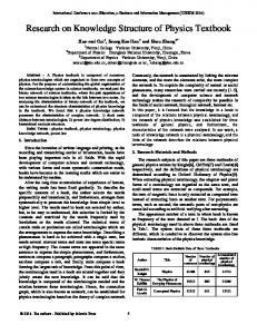
displacement unit oil pipe A hydrostatic pump combustion engine input torque

oil pipe B

hydrostatic motor and displacement unit

cardan shaft connection (back wheel axis)

service brake disc cardan shaft connection (front wheel axis)

Figure 1: Hydrostatic Power-Split CVT

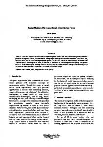
ment pump and a variable displacement motor is developed. The nonlinear state-space system is transformed into a Takagi-Sugeno fuzzy system whereby the nonlinear terms are transferred into weighting functions using the sector nonlinearity approach [17], [21]. The discrete mode changes in the mechanical branch are reflected by switched membership functions. After this, in Section 3, a reduced-order T-S observer design using LMI-based conditions is considered in detail. Finally, it has been shown by simulation studies and experimental results that, first, the proposed T-S model description of the plant is capable to represent the effective nonlinearities and, second, the designed T-S observer can be used for analytical redundancy under varying load conditions. 2. Modeling of Power-split CVTs 2.1. Description and operation principle In power-split CVTs are two parallel paths available, the mechanical and continuously variable path, for power flow from the primary energy source usually a combustion engine to the wheels. There are many diverse technologies to realize the continuously variable path such as mechanical, electrical or hydrostatic. Figure 1 gives an example of a power-split CVT for construction machines with an axle offset between the input and output shaft. Figure 2 shows the associated configuration using a hydrostatic transmission as the continuously variable path. The combustion engine is connected to a hydraulic displacement pump (axial piston type) and also to a spur wheel section with gear ratio i4 (forward direction) or i4 · i4 (backward direction). The pressure level in the hydrostatic transmission between the pump and the motor varies for each individual pipe, depending on the power flow direction. The output speed of the hydrostatic branch 798

pipe A displacement unit

wCE

displacement unit

p

A

wW

wM

i1 hydromotor

p

hydropump

combustion engine

B

i2

C1

pipe B

ia C2

2

2

s

C4

P2

i3 i4

1 P1

1

s

i5

s

1

P3 2

C3 i6 i7 C5

Figure 2: Diagram of the power-split hydrostatic continuously variable transmission is controlled by an electronic control unit (ECU). The displacement elements can be adjusted independently and due to the displacement variation the desired transmission of the variable path is adjusted continuously. The transmission design in Figure 2 offers a large ratio spread using three driving ranges. The first range based on a pure hydrostatic mode, the second and third are power split mode. All shifting points are fully synchronized. The shifting scheme is as follows (see Table 1): In standstill, clutch C1 and C2 are closed. In the first driving range the vehicle is actuated by a pure hydrostatic drive, while the mechanical branch is disconnected from the combustion engine. When the vehicle speeds up, the planetary gears P1 and P2 are accelerated, so that clutch C3 can be closed synchronized at shifting speed. At the end of the second driving range, after the synchronisation point is reached clutch C5 is closed and C1 is opend. The reverse operation is equal, just that instead of C3 the reverse power split clutch C4 is used (see Fig. 2). This setup has high mechanical and control requirements mainly due to the five clutches. As an advantage it offers in both forward and reverse drive high speeds and efficiencies symmetric to standstill [9].

2.2. Modeling of the mechanical power path The key devices in the mechanical power path of the power-split transmission are the three planetary gear sets described as P 1, P 2 and P 3 shown in Fig.2. These planetary gear sets combine the power and constrain the motions of the combustion engine and the hydrostatic motor of the hydrostatic path. Each planetary gear also called epicyclic gearing or sun-and-planet gears has three nodes: the sun gear 1, the carrier gear s, and the ring gear 2. As a result of the direct mechanical connection through gear teeth, the rotational speed of the sun gear ω1 , ring gear ω2 , and carrier gear ωs satisfy the following kinematic relationship at all times ω 1 − ωs (1) iPi ,12 = ω2 − ωs where iPi ,12 denotes the stationary gear ratio of the planetary gearset Pi . Due to the equilibrium of forces at the planetary gear the torque equation between the torque at the sun gear M1 , the ring gear M2 , and carrier gear Ms is valid T 1 + T2 + Ts = 0

C1 0 1 1

C2 0 0 1

C3 1 1 0

C4 0 0 0

C5 1 0 0

1 0

0 0

0 0

1 1

0 1

(2)

And due to the gear ratio iPi ,12 we get the useful relations Ts Ts 1 − iPi ,12 T2 = −iPi ,12 , = iPi ,12 − 1 , = . T1 T1 T1 iPi ,12 (3)

Table 1: Power-split shifting scheme Driving Range 3. Range forward (R3f ) 2. Range forward (R2f ) 1. Range forward/ backward (R1 ) 2. Range backward (R2b ) 3. Range backward (R3b )

.

The further components in the mechanical power path are the hydraulic-actuated clutches C1, ..., C5 and the stationary gears. There are represented in Fig.2 by rectangles where ik = −ωinput /ωoutput , 799

k = 2, ..., 7

(4)

2.3. Modeling of the hydrostatic power path

denotes the fixed ratios. Based on the fact that the shifting points between the first and second, second and third range are fully synchronized the clutches considered as ideal switching elements (i.e. either the clutch C transmits the full torque marked as "1" or no torque marked as "0", see Table 1). By using (1) and (4) the kinematic relationships of the hydrostatic motor speed ωM , the combustion engine speed ωCE and wheel speed ωW for all forward driving ranges are given by

The difference pressure evolution of the hydrostatic power path is described by  10  ˜ x˙ 3 = VmaxP x1 ωP − V˜maxM x2 x4 − kleak x3 CH (12) with x3 := ∆p = pA − pB as the difference pressure between the pipes (see Fig.2), x4 := ωM as the hydrostatic motor speed, CH as the hydraulic capacitances in the elasticity of the connecting pipes, and V˜maxP , V˜maxM as the maximum displacement volume of the pump and motor. The internal leakage oil flow is modeled as a laminar flow resistance, which depends linearly on the difference pressure characterized by the leakage coefficient kleak . Therefore Eq. (12) is nonlinear in the states x2 , x4 as well as nonlinear in the pump speed ωP . Here, some reasonable symmetry assumptions are made. Considering identical hydraulic capacitances in the elasticity of the connecting pipes as leads to an order reduction by one equation for the difference pressure instead of two equations for each pipe [1]. From a system modeling viewpoint the dynamics of the displacement units can be represented by a first order lag element. Consequently, the dynamics of displacement unit of the pump, which is realized as a tiltable swashplate, is governed by

R1 : First driving range (forward and backward) ωW =

iP2 ,12 − iP2 ,12 1 ωM iP1 ,12 − 1 i2 i5 ia | {z }

(5)

[iωM (R1 )]−1

R2f : Second driving range (forward) ωW =  |

1−

1

1



ωCE +

iP1 ,12 i4 i5 ia {z }

iP1 ,12

[iωCE (R2f )]−1

|

(6)

1



1−

1 iP1 ,12



{z

i2 i5 ia }

ωM

[iωM (R2f )]−1

R3f : Third driving range (forward) ωW =

aR3 ia −1 | {z }

[iωCE (R3f

)]−1

ωCE +

b i −1 |R3{za }

[iωM (R3f

ωM

(7)

x˙ 1 = −

)]−1

with aR3

1 − iP3 ,12 1 = , i4 (1 − iP1 ,12 ) i5



bR3 = −

1 iP3 ,12 iP ,12 (1 − iP3 ,12 ) 1 − 1 i2 i6 i7 1 − iP1 ,12 i5

(8)

x˙ 2 = −

 (9)

1 kM x2 + u2 τuM τuM

(14)

with the time constants as τuP respectively τuM and u1 , u2 as the control signals of the hydrostatic pump and motor and the static gains kP , kM . Here, a normalized swashplate angle x1 = αPαP ∈ [−1, 1] and max a normalized bend axis angle x2 = αMαM ∈ [0, 1] max have been introduced. The torque TM of the hydrostatic motor depends on the difference pressure and the bend axis angle controlled by the displacement unit

R1 : First driving range (forward and backward) TW

(13)

whereas the dynamics of the motor according to a bend axis design is described by

The kinematic relations of the 2. and 3. driving range backwards differ from the additional stationary gear i3 (e.g. the term i4 in (6) and (8) have to replaced by i3 · i4 ). The output torque at the wheel as a function of the hydrostatic motor torque can be described as follows:

iP1 ,12 − 1 = ia i5 i2 TM iP2 ,12 − iP1 ,12

1 kP x1 + u1 τuP τuP

TM = V˜maxM x2 x3 ηmh

(10)

(15)

with ηmh as the hydromechanical efficiency of the motor.

R2f : Second driving range (forward)
ia i5 i2 − i2P2 ,12 i2 (iP1 ,12 − 1) TM TW = (iP ,12 + iP1 ,12 ) (1 − iP2 ,12 (1 + iP1 ,12 iP2 ,12 )) | 2 {z }

2.4. Longitudinal vehicle dynamics The longitudinal dynamics of a vehicle with powersplit hydrostatic CVT is governed by the equation of motion 1 h iM (R) iωM (R) V˜maxM 10−4 ηmh x2 x3 x˙ 4 = Jv  iωM (R) i1 ωP − MLw iωM (R) −dv x4 − dv iωCE (R) (16)

iM (R3f )

(11) Remark: Based on the fact that power-split transmissions have a closed chain structure in the powertrain mode (2. and 3. driving range) the combustion engine torque is eliminated by constraint conditions. 800

for R ∈ { R3b , R2b , R1 , R2f , R3f } where ωP = ωCE (see Fig.2) and Jv as the moment of vehicle i1 inertia, dv as the lumped damping coefficient of the powertrain, and TLw as external load torque on wheel. The dependency of the driving range is included by R using the previously defined gearbox ratios (5), (6), (7), (10) and (11).

Third step: The single-argument functions (18) and (19) are combined to the so-called membership functions hi (z) for i = 1, . . . , Nr . They result from the combination of l = 3 sector nonlinearities and 5 different driving ranges with Nr = 2l · 5 = 40 {w11 , w12 } × {w21 , w22 } × {w31 , w32 } × { χ1 , χ2 , χ3 , χ4 , χ5 }

2.5. T-S fuzzy state-space model

using the follwing products

The combination of (12), (13), (14), and (16) to a state-space system with x = [x1 , x2 , x3 , x4 ]T and the following transformation into a T-S fuzzy system [18] is given if first the nonlinearities can be replaced by sector nonlinearities [21], and second, the discrete driving ranges in (16) are represented in the T-S fuzzy framework by singleton sets. However this transformation is not bijective. This means that different T-S fuzzy systems can be derived from a given nonlinear differential equation system. This degree of freedom will be used to meet an essential requirement for the observer synthesis. Yoneyama et al. [23] showed that the separation principle holds if all variables in z can be measured. Otherwise a separate observer design based on LMI-methods is not realizable using the following design approach. Based on this requirement a T-S fuzzy system for reconstructing the pressure difference (⇒ x3 6= zj for j = 1, . . . , l) is carried out in two steps. ¯ P ] as timeFirst step: The pump speed ωP ∈ [ω P , ω variable parameter in (12), (16) and the motor dis¯2 ], x2 > 0 in (14) and placement as state x2 ∈ [x2 , x (12) are bounded. Therefore they can be replaced by a linear combination of the sector functions wj1 and wj2 : f¯j − zj fj (zj ) = f j ¯ + f¯j fj − f j | {z } =wj1 (zj )

zj − f j f¯j − f j | {z }

h1 (z) = w11 (z1 ) · w21 (z2 ) · w31 (z3 ) · χ1 (z4 ) , h2 (z) = w12 (z1 ) · w21 (z2 ) · w31 (z3 ) · χ1 (z4 ) , .. . h40 (z) = w12 (z1 ) · w22 (z2 ) · w32 (z3 ) · χ5 (z4 ) . Finally, all time invariant system matrices of the T-S fuzzy system can be described in a compact form:   0 0 0 − τu1 P   0 0 0 − τu1   M   Ai = 10V˜max ˜max −10 V  −10k leak P M F 0 F  CH 2 1 CH CH 0 a42 a43 − Jdvv (21) with a42 = − a43 =

dv iωM (R) i1 F2 F3 F4 Jv iωCE (R)

1 ˜ VmaxM 10−4 ηmh iM (R) iωM (R) F1 F4 Jv

where F1 ∈ {f 1 , f¯1 }, F2 ∈ {f 2 , f¯2 }, F3 ∈ {f 3 , f¯3 }, and F4 ∈ {χ1 , · · · , χ5 }. By disregarding external loads TLw this leads to the following T-S-fuzzy model for the observer design

(17)

=wj2 (zj )

x˙ =

with f j := min[fj (zj )] and f¯j := max[fj (zj )] whereas f2 (z2 ) = z2 := ωP , 1 f3 (z3 ) := , z3 := x2 x2

(20)

NX r =40

hi (z) Ai x + B u ,

(22)

i=1

with the constant input matrix  k P 0 τ  uP kM  0 τuM B=  0 0 0 0

f1 (z1 ) = z1 := x2 ,

(18)

Second step: The discrete driving ranges are regarded by switching functions, which may be considered in the T-S fuzzy framework as singleton sets in the following form:  1 if R = R3b χ1 (R) = 0 else .. (19) .  1 if R = R3f χ5 (R) = 0 else

    

(23)

and the output equation y = x. 3. Reduced-order observer design 3.1. Observer structure For a nonlinear dynamic system described by the T-S fuzzy model (22) a fuzzy observer can be designed to reconstruct the full state vector. In the considered application we take the advantage of the fact that just one state, the pressure difference, have to be estimated. Hence the order of the observer

for R ∈ { R3b , R2b , R1 , R2f , R3f }.

801

from (26) to get

is reduced by the number of sensed states respectively outputs. This enables, in the following, a reduction of the LMI-based design problem and improved the robustness of the estimated pressure difference against load variation. The state vector is ˜P , α ˜ M , ωM ]T , partitioned into two parts: xa = [ α which is directly measurable, and xb = ∆p, which represents the remaining state variable that has to be estimated. The system matrices of each linear model are accordingly partitioned:        Aiaa Aiab xa B ia x˙ a = + u Aiba Aibb xb B ib x˙ b (24)

y=



E (n−p)×(n−p)

0(n−p)×p





xa xb

e˙ b =

Nr X

Nr X

ATibb P + P Aibb − ATjab N Ti − N i Ajab + 4αP



+ATjbb P + P Ajbb − ATiab N Tj − N j Aiab < 0 ,

(25)

ATibb P + P Aibb − ATiab N Ti − N i Aiab + 2αP < 0 (30) for i, j = 1, ..., Nr where N i = P Li . The matrices P and N i can be found by using convex optimization techniques if the Linear Matrix Inequalities (30) have a feasible solution for a given decay rate α ∈ R+ . The i = 1, . . . , Nr observer gains can then be obtained as Li = P −1 N i . The proof of this theorem follows directly from the proof of the full T-S observer theorem in [21].

ˆb hi (Aibb − Li Aiab ) x hi (Aiba − Li Aiaa ) y

(26)

4. Numerical simulation and experimental validation

i=1

+

Nr X

hi ( B ib − Li B ia ) u

Some numerical simulations are shown in Fig. 3, Fig. 4, Fig. 5 and Fig. 6 to illustrate the function of the CVT transmission in each driving mode. The designed observer is validated by means of a comparsion between a measured x3 and a observed pressure difference x ˆ3 . The measurement was recorded during a test run with a standard wheel loader on a test track. The input signals of the observer law (26) with y = xa = [ x1 , x2 , x4 ]T are supplied by the measured hydropump angle x1 , hydromotor angle x2 and the hydromotor speed x4 . The pressure difference signals are illustrated in Fig. 7 (upper curve) and correspond to a driving cycle with acceleration and deceleration periods showed in the lower curve. The measured pressure difference varies in a full operation range of the hydrostatic power path of a forward vehicle motion. The plot of Fig. 7 shows that the observer is able to reconstruct the pressure difference signal for the purpose of analytical redundancy.

i=1

ˆ b = xc + x

Nr X

hi L i y

i=1

The membership functions hi = hi (z) in (26) and the total number of linear models Nr = 40 are the same as in the original plant model (22). Remark: To get around the difficult of derivative of measurement in reduced-order observer the new state xc is defined.

3.2. LMI-based observer design For the following T-S fuzzy observer design, it is assumed that the fuzzy system model is locally observable, i.e. all (Aibb , Aiab ), i = 1, . . . , Nr pairs are observable. If the estimation error is defined by ˆb eb = xb − x

(27)

5. Conclusion and Outlook

the dynamics of the error are given by substracting x˙ b =

Nr X

hi (z) [Aibb xb + Aiba xa + B ib u ]

(29)

If the error dynamics (29) is stable, the state estimation will converge asymptotically to the real state. An observer with converging state estimation can also be referred to as a stable observer. The stability of the above error dynamics is verified by the following theorem: Theorem: The T-S observer (26) is globally asymptotically stable if a common positive definite matrix P > 0 exists such that

i=1

+

hi (z)hj (z) [Aibb − Li Ajab ] eb

i=1 j=1

with n = 4 and p = 1 wherein E is the identity matrix with ones on the main diagonal and zeros elsewhere. Based on this, the well known reducedorder observer structure [4] for linear time invariant systems and using the idea of Parallel Distributed Compensation (PDC) scheme [20] for nonlinear systems represented by T-S fuzzy models, the nonlinear observer dynamics will then be a weighted sum of the individual linear observers x˙ c =

Nr Nr X X

A model-based analytical redundancy concept for the reconstruction of pressure difference signals in power-split hydrostatic CVTs was presented in this paper. Based on a T-S fuzzy model description of

(28)

i=1

802

clutch 1

1

0 8

10

12

14

16

18

20

0

22 clutch 2

0 2

4

6

8

10

12

14

16

18

20

0

5

10

15

20

25

0

5

10

15

20

25

0

5

10

15

20

25

0

5

10

15

20

25

0

5

10

15

20

25

0.5 0

22

1 1

0.5

clutch 3

clutch 3

6

0.5

0 0

clutch 4

4

0.5

1

0

2

4

6

8

10

12

14

16

18

20

22

0.5 0

1 1

0.5 0 0

clutch 5

2

clutch 4

clutch 2

0 1

2

4

6

8

10

12

14

16

18

20

22

0.5 0

1 0.5

1 clutch 5

clutch 1

1 0.5

0 0

2

4

6

8

10

12

14

16

18

20

22

t [s]

0.5 0 t [s]

Figure 3: Simulation: Clutch control signals {0, 1} for Mode change R1 → R2f → R3f (forward movement)

Figure 5: Simulation: Clutch control signals {0, 1} for Mode change R1 → R2b → R3b (backward movement)

ratio (red) , desired ratio rd (blue) 1.8 ratio (red) , desired ratio rd (blue)

1.6

0.5

1.4 1.2

0

0.8

−0.5 ratio

ratio

1

0.6 0.4

−1

0.2 0 −0.2

−1.5 0

5

10

15

20

25

t [s] −2

0

5

10

15

20

25

t [s]

Figure 4: Simulation: Transmission-ratio tracking (r := ωW /ωCE ) for Mode change R1 → R2f → R3f (forward movement)

Figure 6: Simulation: Transmission-ratio tracking (r := ωW /ωCE ) for Mode change R1 → R2b → R3b (backward movement)

the nonlinear plant a reduced-order T-S observer was designed by solving an appropriate LMI condition. It was shown e.g. in [21] that those designed observers guarantee a global asymptotically stable error dynamics. The reduced-order T-S fuzzy observer was experimentally validated by means of a comparison between the measured and the reconstructed pressure difference signal. The presented figures clearly show that the observer is able to reconstruct the pressure difference signal for the purpose of analytical redundancy. This is the essential step for developing a model-based fault diagnosis system for mobile working machines. In a next step we will design further observers for monitoring also the speed of the hydrostatic motor. Based on this a dedicated observer scheme [11] for a sensor fault diagnosis and identification system (FDI) should be designed and tested on a real test vehicle.

References [1] H. Aschemann, J. Ritzke, and H. Schulte. Model-Based Nonlinear Trajectory Control of a Drive Chain with Hydrostatic Transmission International Conference on Methods and Models in Automation and Robotics (MMAR), Miedzyzdroje, Poland, 2009. [2] IEC 61508, Functional safety of electrical / electronic / programmable electronic safetyrelated systems. 2001. [3] M. Erikkilä. Model-based Design of Power-Split Drivelines, PhD thesis, Tampere University of Technology, Finland, 2009. [4] G. F. Franklin, J. D. Powell, and A. EmamiNaeini. Feedback Control of Dynamic Systems. Addision-Wesley Publishing Company, second edition, 1991. 803

∆p

∆p [bar]

[14] M. Sannelius. On complex hydrostatic transmissions. PhD thesis, Linköping Studies and Technology, No. 569, Linköping, Sweden, 1999. [15] S. M. Savaresi, F. L. Taroni, F. Previdi, and S. Bittanti. Control System Design on a PowerSplit CVT for High-Power Agricultural Tractors. IEEE Transactions on Mechatronics, 9(3): 569–579, 2004. [16] H. Schulte. Modeling of Hydrostatic Transmissions considering leakage losses. In IFAC Workshop on Advanced Fuzzy-Neural Control Proceedings, Valenciennes, France, 2007. [17] H. Schulte and P. Gerland. Observer Design using T-S Fuzzy Systems for pressure estimation in hydrostatic transmissions 9th International Conference on Intelligent Systems Design and Applications, Pisa, Italy, 2009. [18] T. Takagi and M. Sugeno. Fuzzy identification of systems and its application to modelling in control. IEEE Transactions on System, Man and Cybernetics, 15(1):116–132, 1985. [19] K. Tanaka, T. Ikeda, and H. O. Wang. Fuzzy regulators and fuzzy observers: Relaxed stability conditions and LMI-based designs. IEEE Transactions on Fuzzy Systems, 6(2):1–16, 1998. [20] K. Tanaka and M. Sugeno. Stability analysis and design of fuzzy control systems. Fuzzy Sets and Systems, 45:135–156, 1992. [21] K. Tanaka and H. Wang. Fuzzy Control Systems Design and Analysis. John Wiley & Sons, New York, Chichester, 2001. [22] J. Wochnik. Modellbildung und nichtlineare Regelung dieselhydraulisch angetriebener Flurförderfahrzeuge (in German). PhD thesis, GHUni Duisburg, Germany, 1992. [23] J. Yoneyama, M. Nishikawa, H. Katayama, and A. Ichikawa. Output stabilization of takagisugeno fuzzy systems. Fuzzy Sets and Systems, 111(2):253–266, 2000. [24] Z. Zou, Y. Zhang, X. Zhang, and W. Tobler. Ratio Control of Traction Drive Continuously Variable Transmissions. In Proceedings of the American Control Conference, Chicago, Illinois, June 2000

measured pressure difference estimated pressure difference

500

0

−500

20

30

40

50

60

70

80

90

t [s] nw

measured wheel speed simulated wheel speed

50

w

n [u/min]

40 30 20 10 0

20

30

40

50

60

70

80

90

t [s]

Figure 7: Measured and estimated pressure difference during Driving Range Mode R1 (forward movement)

[5] X. Guo, S. Yuan, and J. Hu. The design and numerical simulation of a hydro-mechanical continuously variable transmission system for heavy-duty vehicles. International Fluid Power Conference, Aachen, Germany, 2006. [6] K. Huhtala. Modelling of Hydrostatic Transmissions - Steady State, Linear and Nonlinear Models. PhD thesis, Tampere, Finland, 1996. [7] J. Lennevi, K. E. Rydberg, and J. O. Palmberg. Microprocessor control of hydrostatic transmissions adapting to driving conditions. In 11th Aachener Fluidtechnisches Kolloqium, Aachen, Germany, 1994. [8] C. J. Lopez-Toribio, R. J. Patton, and S. Daley. Takagi-Sugeno Fuzzy-Tolerant Control of an Induction Motor. Neural Computing and Application, 9:19–28, 2000. [9] S. Mutschler. Economic Evaluation of Hydrostatic Drive Train Concepts for Mobile Machinery In 6th International Fluid Power Conference Dresden, Aachen, Germany, 2008. [10] M. Oudghiri, M. Chadli, and A. E. Hajjaji. Control and Sensor Fault-Tolerance of Vehicle Lateral Dynamics. In Proceedings of the 17th World Congress IFAC, pages 123–128, 2008. [11] R. J. Patton, P. M. Frank, and R. N. Clark. Fault diagnosis in dynamics systems theory and application. Prentice-Hall International, UK, 1989. [12] K. Renius and R. Resch. Continuously Variable Tractor Transmissions. ASAE Publication, No. 913C0305, 2005. [13] K. E. Rydberg. On performance optimization and digital control of hydrostatic drives for vehicle applications. PhD thesis, Linköping Studies and Technology, No. 99, Linköping, Sweden, 1983. 804