ogy that is based on graphs or, more generally, sub- ... derivation of the backstepping technique, where one ... ular section of the control bundle (see [10].) ...
Control-Transverse and Graph Dynamics and Relations to Backstepping EFTHIMIOS KAPPOS Department of Applied Mathematics, University of Sheffield, Sheffield S3 7RH ENGLAND
Abstract: In this paper we examine the transverse geometry of control-affine systems. We point out the importance the singular set and of dynamics defined on submanifolds that are transverse to the control distribution. This setting is then used to compare the backstepping methodology for strict-feedback systems with our more general approach to nonlinear control design. Keywords: Nonlinear control design, backstepping, singular set, Lyapunov functions
1
Introduction
Let us compare the two control-affine systems: ½ x˙ 1 = x2 − f1 (x1 ) x˙ 2 = u ½
x˙ 1 x˙ 2
= =
f1 (x1 , x2 ) u
cation of backstepping, no such assumption is necessary in the approach we take through transverse dynamics. (1)
(2)
The former system belongs to the class of control systems in strict feedback form, which allows the backstepping methodology to be applied. The latter is in some natural sense a local normal form for arbitrary control-affine systems (see section 2.) One can ask the question: When can we ascertain that the general system of equation (2) is feedback equivalent to the more restrictive form of equation (1)? Note that we only assume that (x1 , x2 ) ∈ R(n−m) × Rm for some 0 < m < n in equation (2), while in the backstepping context x1 and u must be one-dimensional (the more general form is given in equation (4).) The key idea is to focus attention on the singular set of the control system, the set where the control directions belong to a subspace of the tangent space, rather than an affine subspace. We study the geometry of singular sets in section 2. We also present a novel control design methodology that is based on graphs or, more generally, submanifolds that are transverse to the control distribution. This crucial point is somewhat obscured in the derivation of the backstepping technique, where one has to pretend that a state is a ‘virtual’ control. Our approach, like backstepping, benefits from a decomposition into dynamics transverse to the control directions and dynamics in the control directions. Note that, while one assumes a single control in the appli-
2
Graphs and Control Transverse Dynamics
In Nonlinear Control Theory ([19], [20]), one most commonly studies control-affine systems of the form x˙ = f (x) +
m X
ui gi (x) ,
x∈V ,
n ≥ m > 0, (3)
i=1
with V some open subset of Rn and f, g1 , . . . , gm smooth vector fields in V ⊂ Rn . Such control-affine systems can be considered as approximations of the more general control systems x˙ = f (x, u) near a regular section of the control bundle (see [10].) Even if the state space is a manifold M n , we shall be working mostly in a neighbourhood of some point, and will thus assume that we have used local coordinates to write the system in an open subset V of Rn . Definition 1. The control distribution D is the linear span of the vector fields {g1 , . . . , gm }. The set of feedback controls Γ(D) is the set of smooth section of the sub-bundle D ⊂ T M . Recent practical control methodologies rely heavily on rather special forms for the control dynamics. A main example is the backstepping methodology, which, in its basic form, assumes the strict feedback form x˙ 1 = x2 − f1 (x1 ) x˙ 2 = x3 − f2 (x1 , x2 ) ··· ··· ··· (4) x ˙ = x − f (x , . . . , x ) n−1 n n−1 1 n−1 x˙ n = u
Now there is a straightforward way to express the general control-affine system (3) above in a more useful form. The following is a basic definition:
has constant-rank m in an open, star-shaped domain of Rn containing V .
It is a simple fact from Algebraic Topology that Definition 2. The singular set Σ of the controlthe control distribution D ⊂ T Rn |V forms a trivial n affine system is the subset of R vector bundle, in other words there is a diffeomorphism Σ = {x ∈ V ; f (x) ∈ img(x)} D ' V × Rn . This definition can be easily modified for the case when the control is not unbounded: it is the set of Proposition 1. In a relatively compact subset of V , all points of the state space where the ‘state dynamthe control affine system of equation (3) is feedback ics’ f (x) lies in the control set g(x)U , where g is the equivalent to the system m (n × m) matrix of controls and U ⊂ R is the con½ trol set. The singular set is a fundamental object in x˙ 1 = f1 (x1 , x2 ) the study of nonlinear control systems. For a start, (5) x˙ 2 = g2 (x1 , x2 )u, all possible equilibrium points of all possible control dynamics lie in Σ: where the square m×m matrix is nonsingular, so that Lemma 1. The singular set contains all equilibrium we can further simplify the above system by setting points of any control dynamics and is generically a g2 = Im (thus obtaining the system of equation (2). manifold of dimension equal to the dimension of the control, m. Generic here means for a residual set in This result says that, when considering control X (V )n+1 the set of (n + 1)-tuples of vector fields on dynamics, one can decompose the state into the ‘conV. trol directions’ and the directions transverse to the From now on, we shall make it an assumption that control. In particular, one can consider submanifolds Σ is indeed a manifold of the appropriate dimension: and foliations transverse to the control distribution D and define on these geometric objects dynamics, Assumption 1. We assume that the singular set is which will be called control-transverse dynamics. By varying these transverse manifolds or foliations, an m-dimensional submanifold: Σm ⊂ V ⊂ Rn . we vary the control-transverse dynamics. Let us give But the role of the singular set is revealed best some more detail (also see references [14], [12], [10], when considering the stabilization problem in [13].) control—see Proposition 4 below. This is the probWe shall consider (local) coordinate systems such lem of the existence of a control strategy that yields that the control distribution is constant. We canoncontrol dynamics with, at least locally, an asymptotically identify Rn with each of its tangent spaces ically stable equilibrium. Tx Rn . We have the direct sum The subject of stabilization has witnessed considerable development (see for example [1]), yet still Rn = E n−m ⊕ Dm lacks a good constructive methodology. The backstepping technique, which appeared in the midnineties, is explicitly a stabilization method. How- and we write x = (x1 , x2 ) x1 ∈ E, x2 ∈ D and, by ever, it had to rely on the control system taking a the above identification also x˙ = (x˙ 1 , x˙ 2 ). The main geometrical objects on which we shall rather special form. define dynamics are submanifolds N n−m and foWe shall examine the singular set for controlliations F transverse to the sub-bundle D and of affine systems, and see how they take a special form complementary dimension. This means, for a subin the case of strict feedback systems in the next secmanifold N , that tion. The main interest is when the set V is a neighbourhood of a point p ∈ Σ, a point that we wish to stabilize, for example. For now, we proceed with the Tx N ⊕ Dx = Tx Rn , ∀x ∈ N normal form for control-affine systems. Assumption 2. We assume that the control distribution, defined point-wise by Dx = span{g1 (x), . . . , gm (x)},
and similarly for each leaf of F. Locally, control-transverse manifolds are in a oneto-one correspondence with graphs of functions, as follows:
Proposition 2. Let p ∈ M n and assume the conCompare this with the backstepping approach for trol distribution is trivial in a neighbourhood of the the system (1): this considers the state component point p. We can assume moreover that we decom- x2 as a virtual control and takes pose T M |W into D ⊕ E, D, E fixed subspaces. Then x2 = f1 (x1 ) − αx1 , for every submanifold N n−m transverse to D at p (and hence locally), we can find a neighbourhood for example, which yields a stable subsystem. A LyaW ⊃ N 3 p and a function punov function for the subsystem is then extended to the whole state by defining ψ:E→D such that graphψ = N |W .
V (x1 , x2 ) =
1 2 1 2 x + (x2 − f1 (x1 ) − αx1 ) . 2 1 2
Now, given the normal form of the Lemma, choosThis step-by-step approach can easily extend to the ing a control-transverse submanifold or equivalently, full system of the form of equation (4.) choosing, locally, a function ψ : E → D ' Rm (E ⊂ Rn−m ) we can define the dynamics of the system x˙ 1 = f1 (x1 , ψ(x1 )). (6) Proposition 3. There is a choice of a smooth feedback control in a tubular neighbourhood of a controltransverse manifold N that makes the manifold invariant under the control flow. The dynamics thus obtained on N are topologically orbitally equivalent to the dynamics on the graph of a suitable ψ as above in equation (6). Proof. Since we have that the manifold is locally the graph of a function ψ : E → D, we can make it invariant by choosing u = x˙ 2 =
∂ψ ∂ψ x˙ 1 = f1 (x1 , ψ(x1 )). ∂x ∂x
Since we can control the D-directions, we can then extend the control to a tubular neighbourhood of N such that N is a hyperbolic invariant set (we can make N asymptotically stable, for example.) The last part just says that the dynamics on N are given by x˙ 1 = f1 (x1 , ψ(x1 )),
3
Singular set geometry
Given a control-affine system in the ‘normal form’ of equation (5), the singular set is obtained by setting f1 to zero: Σ = {x ∈ V ; f1 (x1 , x2 ) = 0}. (so we have (n − m) equations in n variables.) Here is the relevant result from Differential Geometry: Proposition 5. Suppose that zero is a regular value of f1 . Then Σ is an m-dimensional smooth submanifold. In fact, the distribution ker df1 is then regular nearby, and hence, since it also integrable, we can find a foliation by the level sets of f1 near the value 0. The proof is standard and ultimately rests on the implicit function theorem (see, for example, Conlon [3].)
Singular sets and control distribution We saw that submanifolds that are transverse to the singular set play a special role in control theory. Proposition 4, for example, gave a necessary and sufficient condition for smooth stabilization in terms of a controltransverse manifold with stable dynamics. But there which is clear. are stronger connections that bring us closer to the linear system idea of controllability. More specifHere is an important result that uses the control- ically, we assert that what is of more interest, from the dynamical viewpoint, in the strict feedback form transverse dynamics notion. is not that we can derive a stabilizing feedback, but Proposition 4. The control-affine system is that we can transform the system to a linear consmoothly stabilizable to the point p ∈ Σ if and only if trollable form! Now the singular set for the strict feedback form there is an (n − m)-dimensional submanifold transverse to D and containing p such that the invariant of the backstepping method is found by setting x˙ 1 = x˙ 2 = . . . = x˙ n−1 = 0 in the system (4), in other dynamics are locally asymptotically stable
words, setting x2 x3 ··· xn
4 = = ··· =
Singular sets in the plane
f1 (x1 ) f2 (x1 , x2 ) ··· fn−1 (x1 , . . . , xn−1 )
In Figure 1, we give some typical positions for the singular set in the plane of a system with m = 1 in (7) relation to the control distribution D, which is taken to be vertical, D =< e2 > in the figure (where, as usual, we have identified R2 ' T0 R2 . The last equation certainly gives a graph transverse First, we fix a point p ∈ Σ. We have the following to D =< en >, in agreement with the Proposition. cases: Successive equations give graphs—and hence transverse manifolds— on the previous graph until we get 1. The singular set is a complement of D at p to the two-dimensional one given by x2 = f1 (x1 ), so (Fig.1(A)): that the idea of ‘virtual controls’ seems a natural one. In the design process, we take these graphs in the reTp Σ + Dp = Tp R2 verse order, i.e. in the order they are listed in the and 0 is a regular value of the function f1 . This equation above, and use graph dynamics in the manis the generic case and also the one assumed ner we described to get a stable system overall. What in the backstepping approach. However, let us is as important, though, is that if we forget the stabinote that it is possible to choose graphs with arlization issue, we can obtain the transformed system bitrary dynamics: stable, unstable, semi-stable. (a ‘feedback-equivalent system) As a result, we can make p not only into a x ˙ = x locally asymptotically stable equilibrium, but 1 2 = x3 x˙ 2 also a repeller or a saddle point in the plane. ··· ··· ··· (8) 2. We have that Tp Σ = D, but 0 is still a regular x ˙ = x n−1 n value of f1 (Fig.1(B) and (C)). If f1 (x1 , ²) · x1 x˙ n = u is negative,then it is still possible to stabilize Let us turn now to the singular set for the systhe system, by choosing a graph as shown. If tem (2). In order to be able to compare with the the product is positive, then we cannot achieve strict feedback case, we shall work in the case when stable local dynamics using smooth feedback. D is one-dimensional. Fix a point p ∈ Σ. By our However, it may still be possible to achieve staassumption, the one forms df1 , . . . , dfn−1 are linearly ble local dynamics by non-smooth feedback–by independent at, and near, p. In general, D and Σ picking a graph with infinite slope in Figure will not be tangent at p. The derivative matrix for 2(C). This is the case highlighted by Kawski the strict feedback system is in [15]. df 1 3. We have that Tp Σ = D, but now 0 is not a reg1 0 ··· 0 dx ∂f21 ∂f2 ular value of f1 (Fig.1(D)). The range of dy1 ··· 0 df = ∂x1 ∂x2 (9) namics we can achieve is now limited and sta··· ··· ··· ··· ··· ∂fn−1 bilization is not possible (the semi-stable one· · · · · · · · · ∂xn−1 1 dimensional dynamics shown can be extended to saddle-node dynamics in the plane, for exand we note that this linear map preserves the stanample.) n dard flag in R 0 = V 0 ⊂ V 1 ⊂ V 2 ⊂ · · · ⊂ V n = Rn , 1
5
Conclusions
2
where V =< en >, V =< en−1 , en > etc. A general position argument will easily show that we can at least get a transverse graph
This paper promulgates an approach to nonlinear control dynamics through the dynamics defined on submanifolds and foliations transverse to (and of complementary dimension) the control distribution xn−1 = f˜n−1 (x1 , . . . , xn−1 ), D =< g >. The backstepping method certainly by assuming, without loss of generality, that makes use of this idea, indirectly, although it does dfn−1 (D) 6= 0 and appealing to the implicit function not give prominence to the transverse geometry, as theorem. It is not clear how this can be continued. we do.
References [1] [2]
[3] [4]
[12] E. Kappos, “Local Controlled Dynamics,” in D. Owens, A. Zinober eds.: Nonlinear and Adaptive A. Bacciotti: Local Stabilizability of Nonlinear Control, Springer, 2003. Control Systems, World Scientific, 1992. [13] E. Kappos, “A Condition for Smooth StaR. Brockett, “Asymptotic Stability and Feedbilization,” Proc. of the MCSS Conference, back Stabilization,” in R. Brockett, R. MillP´erpignan, 2000. mann, H. Sussmann eds: Differential Geometric Control Theory, Birkh¨auser, 1983, pp.181–191. [14] E. Kappos, “The Role of Morse-Lyapunov Functions in the Design of Nonlinear Global FeedL. Conlon: Differentiable Manifolds, Birkh¨auser, back Dynamics,” in A. Zinober ed.: Variable Boston, 2001. Structure and Lyapunov Control, Lect. Notes in J.M. Coron, “A Necessary Condition for FeedControl and Infor. Sciences 193, Springer, 1994, back Stabilization,” System and Control Letters pp.249–267. 14, 1990, pp.227–232.
[15] M. Kawski, “Stabilization of nonlinear systems in the plane,” Systems Control Lett. 12-2, 1989, [6] A.T. Fomenko: Variational Problems in Topolpp.169–175. ogy, Gordon and Breach, 1990. [16] H. Khalil: Nonlinear Systems, 2nd Ed. Prentice [7] S.-T. Hu: Homotopy Theory, Academic Press, Hall, 1996. 1959. [5] J. Dugundji: Topology, Allyn and Bacon, 1966.
[8] E. Kappos, “The Conley index and Global Bi- [17] M. Krsti´c, P. Kokotovi´c and I. Kanellakopoulos: Nonlinear and Adaptive Control Design, Wiley, furcations, Part I: Concepts and Theory,” Int.J. New York, 1995. Bif. and Chaos, 5–4, 1995, pp.937–953. [9] E. Kappos, “The Conley index and Global Bifur- [18] J. Milnor: Topology from the Differentiable cations, Part II: Illustrative Applications” Int.J. Viewpoint, The University Press of Virginia, Bif. and Chaos, 6–12B, 1996, pp.2491–2505. 1965. [10] E. Kappos: Global Controlled Dynamics, book manuscript, 2003. [11] E. Kappos, “A Global, Geometrical, InputOutput Linearization Theory,” IMA J. Math. Con. and Info., 9–1, 1992, pp.1–21.
[19] S. Sastry: Nonlinear Systems: Analysis, Stability and Control, Springer, 1999. [20] M. Vidyasagar: Nonlinear System Theory, Prentice–Hall, 1978.
+
_
_
_
+
+ +
_
_
A
B
+
+ +
_+ +
C
+
D
Figure 1: Singular sets in the plane and some transverse dynamics.