Controlled Total Variation regularization for inverse problems
arXiv:1110.3194v1 [cs.CV] 14 Oct 2011
Qiyu Jina,b Ion Gramaa,b Quansheng Liua,b
[email protected]
[email protected]
[email protected] a Universit
de Bretagne-Sud, Campus de Tohaninic, BP 573, 56017 Vannes, France b Universit
Europenne de Bretagne, France
Abstract This paper provides a new algorithm for solving inverse problems, based on the minimization of the L2 norm and on the control of the Total Variation. It consists in relaxing the role of the Total Variation in the classical Total Variation minimization approach, which permits us to get better approximation to the inverse problems. The numerical results on the deconvolution problem show that our method outperforms some previous ones.
Key words: Inverse problem, deconvolution, Total Variation, denoising.
1
Introduction
Environmental effects and imperfections of image acquisition devices tend to degrade the quality of imagery data, thereby making the problem of image restoration an important part of modern imaging sciences. Very often the images are distorted by some linear transformations. In this paper, we consider the reconstruction of the unknown function f from the following inverse problem: Y (x) = Kf (x) + ǫ(x), x ∈ I = {0, ..., N − 1}2 ,
(1) 2
where Y is the observed data, K is a continuous linear operator from RN to RM , f is the original image, ǫ is a white Gaussian noise of mean 0 and variance σ 2 , N > 1 and M > 1 are integers. We want to recover the original image f starting from the observed one Y . When the operator K is formulated as a convolution with a kernel, this inverse problem reduces to the image deconvolution model in the presence of noise. Of particular interest is the case where the operator K is the convolution with the Gaussian kernel: X Kf (x) = g ∗ f (x) = g (x − y) f (y) , x ∈ I, (2) y∈I
1
where g (y) =
1 − 2σ12 |y|2 e b , 2πσb2
(3)
and σb > 0 is the standard deviation parameter. This type of inverse problems appears in medical imaging, astronomical and laser imaging, microscopy, remote sensing, photography, etc. The problem (1) can be decomposed into two sub-problems: the denoising problem Y (x) = u(x) + ǫ(x), x ∈ I
(4)
and the possibly ill-posed inverse problem u (x) = Kf (x) , x ∈ I.
(5)
Thus, the restoration of the signal f from the model (1) will be performed into two steps: firstly, remove the Gaussian noise in the model (4); secondly, find a solution to the problem (5). For the first step, there are many efficient methods, see e.g. Buades, Coll and Morel (2005 [2]), Kervrann (2006 [13]), Lou, Zhang, Osher and Bertozzi (2010 [14]), Polzehl and Spokoiny (2006 [17]), Garnett, Huegerich and Chui (2005 [9]), Cai, Chan, Nikolova (2008 [4]), Katkovnik, Foi, Egiazarian, and Astola ( 2010 [12]), Dabov, Foi, Katkovnik and Egiazarian (2006 [3]), and Jin, Grama and Liu(2011 [11]). The second step consists in finding a convenient function fe satisfying (exactly or approximately) Kfe − u = 0, (6) where u is obtained by the denoising algorithm of the first step. To find a solution to the ill-posed problem (6), one usually considers some constraints which are believed to be satisfied by natural images. Such constraints may include, in particular, the minimization of the L2 norm of fe or ∇fe and the minimization of the Total Variation. The famous Tikhonov regularization method (1977 [19] and 1996 [8]) consists in solving the following minimization problem: fb(x) = arg min kfek22
(7)
kKfe − uk22 = 0.
(8)
fe(x)
subject to
Using the usual Lagrange multipliers approach, this leads to 1 fb = arg min kfek22 + λkKfe − uk22, e 2 f where λ > 0 is interpreted as a regularization parameter. An alternative regularization (1977 [1]) is to replace the L2 norm in (7) with the H1 semi-norm, which leads to the well-known Wiener filter for image deconvolution: fb = arg min k∇fek22 fe
2
(9)
subject to (8), or, again by the Lagrange multipliers approach, 1 fb = arg min k∇fek22 + λkKfe − uk22 . 2 fe
(10)
where λ > 0 is a regularization parameter. The Total Variation (TV) regularization called ROF model (see Rudin, Osher and Fatemi [18]), is a modification of (9) with k∇fek22 replaced by k∇fek1 : fb = arg min k∇fek1 fe
(11)
subject to (8), or, again by the Lagrange multipliers approach, 1 fb = arg min k∇fek1 + λkKfe − uk22 . 2 fe
(12)
where λ > 0 is a regularization parameter. Due to its virtue of preserving edges, it is widely used in image processing, such as blind deconvolution [6, 10, 15], inpaintings [5] and super-resolution [16]. Luo et al [14] composed TV-based methods with Non-Local means approach to preserve fine structures, details and textures. The classical approach to resolve (12), for a fixed parameter 0 < λ < +∞, consists in searching for a critical point fe characterized by L(fe) + λK∗ (Kfe − u) = 0,
(13)
∇f , |∇f | being the Euclidean norm of the gradient ∇f. The usual where L(f ) = ∇ |∇f | technique to find a solution fe of (13) is the gradient descent approach, which employs the iteration procedure fk+1 = fk − h (Lfk + λK∗ (Kfk − u)) , (14)
where h > 0 is a fixed parameter. If the algorithm converges, say fk → fe, then fe satisfies the equation (13). However, this algorithm cannot resolve exactly the initial deconvolution problem (6), for, usually, L(fe) 6= 0, so that, by (13), Kfe − u 6= 0. This will be shown in the next sections by simulation results. In this paper, we propose an improvement of the algorithm (14), which permits us to obtain an exact solution of the deconvolution problem (6) when the solution exists, and the closest approximation to the original image when the exact solution to (6) does not exist. Precisely, we shall search for a solution fe of the equation K∗ (Kfe − u) = 0, with a small enough TV. Notice that the last equation characterizes the critical points fe of the minimization problem minfe kKfe − uk22 which, in turn, whose minimiser gives the closest approximation to the deconvolution problem (6), even if it does not have any solution. In the proposed algorithm, we do not search for the minimization of the TV. 3
Instead of this, we introduce a factor in the iteration process (14) to have a control on the evolution of the TV. Compared with the usual TV minimization approach, the new algorithm retains the image details with higher fidelity, as the TV of the restored image is closer to the TV of the original image. Our experimental results confirm this point, and show that our new algorithm outperforms the recently ones proposed in the literature that are based on the minimization problems (10) and (12).
2 2.1
A new algorithm for the inverse problem Controlled Total Variation regularization algorithm
We would like to find fe satisfying the deconvolution equation (6) with a small Total Variation. Since an exact solution to (6) may not exist, instead of the initial problem we consider the minimization problem min kKfe − uk22 . fe
(15)
This leads us to search for critical points fe characterized by the equation K∗ (Kfe − u) = 0,
(16)
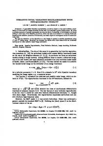
whose TV is small enough. As explained in the introduction, the usual algorithm (14) (classic TV) does not lead to a solution of (16) if it exists. In fact, we have observed by simulation results that usually kLfk k1 does not converge to 0 with k → +∞, so that K∗ (Kfk − u) does not tend to 0 neither. For example taking ”Lena” as test image blurred by the Gaussian convolution kernel (3) with standard deviation σb = 2, the value of ||Lfk ||1 increases (see Figure 1 (b), where the classical TV curve correspond to the dashed line) as log k increases. On the other hand, Figure 1 (c) shows that the value of ||K∗ (Kfk − u)||1 decreases when log k increases in the interval [0, 3], but it remains bounded from below by e8 − 1 ≈ 2980 and does not decrease towards 0 when log k varies in the interval [3, 8]. These considerations lead us to the following modified version of (14): fk+1 = fk − h (θk Lfk + λK∗ (Kfk − u)) ,
(17)
where h > 0, λ > 0 are as in (14) and θk > 0 is a sequence decreasing to 0. We shall use θk = θk , for some θ ∈ (0, 1). This ensures that, if the algorithm converges, say fk → fe, then K∗ (Kfe − u) = 0. (18) Notice that, compared with the initial algorithm (14), we put a small weight θk to the TV in the minimization problem (12), thus diminishing the role of this term in the minimization, in order to get an exact solution to the ill-posed problem (18). Here we do not search for the minimization of the TV, but just for a control on the TV. The control 4
of TV rather than the minimization of TV permets us to better preserve image edges and details. The new algorithm given by (17) will be called Controlled Total Variation regularization algorithm (CTV). We show by simulations that the new algorithm improves the quality of image restauration. In Figures 1 and 2, we see that the TV of the restored image by the proposed CTV algorithm is larger than that of the restored image by the classical TV minimization approach, but closer to the TV of the original image. This also shows that in the classical TV minimization algorithm the TV of the restored image is too small and that the classical approach may not give the best solution. On the other hand, by simulation we have also seen that the TV in the iterative process (17) cannot be suppressed completely, i.e. we cannot take θk = 0. In the case of the Gaussian blur kernel, Figure 1 (c) shows that values of ||K∗ (Kfk −u)||1 computed by the new algorithm CTV and those by the classical TV algorithm are nearly the same, when log k varies in the interval [0, 3]. However, for log k varying in the interval [3, 8], the values of ||K∗ (Kfk − u)||1 by the classical TV algorithm remain constant, while those computed by our algorithm continue to decrease to 0. Accordingly, we see in Figure 1 (d) that the PSNR (the definition of PSNR see Section 3.1) values by the classical TV algorithm and by the new proposed one, are almost the same for log k varying in the interval [0, 3], imitating the evolution of ||K∗ (Kfk − u)||1 ; however, for log k varying in the interval [3, 8], the PSNR value by the classical TV algorithm does not increase any more, while the corresponding PSNR by the new algorithm continues to rise. In the case of 9 ×9 box average blur kernel, Figure 2 displays similar evolutions as those of the Gaussian blur kernel case. Figure 3 shows the images restored by our method and the classical TV method respectively. Our method keeps much more details of the image than the classical TV method.
2.2
Direct Gradient Descent 2
2
Suppose that K a linear operator from RN to RN . To solve the deconvolution problem (6), inspired by (17), we can also consider the following modified version, that we call Direct Gradient Descent (DGD): fk+1 = fk − h (θk Lfk + λ(Kfk − u)) ,
(19)
where 0 < θk → 0. If the algorithm converges, say fk → fe, then fe satisfies exactly the equation (6). Therefore we could expect that this algorithm gives a better solution to the deconvolution problem. By simulations, this is shown to be the case when K is the Gaussian blur kernel and the noise is absent. In this case we find that the DGD approach restores the blurred image more efficiently than classical TV and the CTV regularization approaches introduced above. The results of comparison between the classical TV, CTV and DGD are displayed in Figures 1 and 4. However, our simulations also show that the algorithm DGD is very sensible to the noise and often may not converge. For example, when K is the Gaussian blur kernel, but in the presence of the noise, the method does not give good restoration results; when K 5
Classical TV and CTV (Gaussian blur kernel) 15
12
+ 1 )
10
8
log ( || L f
k
||
1
TV ( f k )
10
5 Classical TV CTV Original image blurred image 0
0
1
2
3
4
5
6
7
8
6
4
2 Classical TV CTV 0
9
0
1
2
3
4
log k
5
6
7
8
9
log k
(a)
(b)
12
42
40
10
38 8 PSNR
36 6
34
log ( || K
*
( K f k − u ) || 1 + 1 )
Classical TV CTV
4 32 2
0
30
0
1
2
3
4
5
6
7
8
28
9
log k
Classical TV CTV 0
1
2
3
4
5
6
7
8
9
log k
(c)
(d)
Figure 1: Comparison between classical TV and CTV. The test image ”Lena” is convoluted with Gaussian blur kernel of standard deviation σb = 1. We choose h = 0.1, λ = 1, max Iter = 3000 and θ = 0.98. (a) The evolution of T V (fk ) as a function of log k. (b) The evolution of log(||Lfk ||1 + 1) as a function of log k. (c) The evolution of log(||K∗ (Kfk − u)||1 + 1) as a function of log k, (d) The evolution of PSNR value as a function of log k.
6
Classical TV and CTV (box average blue kernel) 15
12
+ 1 )
10
8
log ( || L f
k
||
1
TV ( f k )
10
5 Classical TV CTV Original image blurred image 0
0
1
2
3
4
5
6
7
8
6
4
2 Classical TV CTV 0
9
0
1
2
3
4
log k
5
6
7
8
9
log k
(a)
(b)
14
34 Classical TV CTV 32
10 30 PSNR
8
6
28
log ( || K
*
( K f k − u ) || 1 + 1 )
12
26 4 24
2
0
Classical TV CTV 0
1
2
3
4
5
6
7
8
22
9
log k
0
1
2
3
4
5
6
7
8
9
log k
(c)
(d)
Figure 2: Comparison between classical TV and CTV. The test image ”Lena” is convoluted with 9 × 9 box average blur kernel. We choose h = 0.1, λ = 1, max Iter = 3000 and θ = 0.998. (a) The evolution of T V (fk ) as a function of log k. (b) The evolution of log(||Lfk ||1 + 1) as a function of log k. (c) The evolution of log(||K∗ (Kfk − u)||1 + 1) as a function of log k, (d) The evolution of PSNR value as a function of log k.
7
Restoration results with classical TV and CTV
(a) CTV, PSNR= 42.05db
(b) classical TV, PSNR= 34.18db
(c) CTV, PSNR= 32.06db
(d) classical TV, PSNR= 28.33db
Figure 3: (a) and (b) are the images restored from the test image ”Lena” convoluted with Gaussian blur kernel with σb = 1 by our method and by classical TV method respectively. (c) and (d) are the images restored from the test image ”Lena” convoluted with 9 × 9 box average blur kernel by our method and by classical TV method respectively.
8
is the 9 × 9 box average kernel, the algorithm diverges and the restoration results are not good with or without noise (see Figure 5). Notice also that the CTV regularization approach applies even if the linear operator K 2 is from RN to RM , where M is possibly different from N 2 , contrary to the DGD approach which applies only when M = N 2 . The aforementioned arguments show that the CTV regularization approach (17) should be proffered to the Direct Gradient Descent algorithm (19), especially when the blurring is accompanied with a noise contamination.
3
Numerical simulation
3.1
Computational algorithm
In this section we present some numerical results to compare different deblurring methods. We shall use CTV regularization algorithm to restore several standard blurred and noisy images and compare it to the Tikhonov + NL/H1 (Tikhonov regularization followed by a Non-Local weighted H 1 approach) and Tikhonov + NL/TV (Tikhonov regularization followed by a Non-Local weighted TV approach) algorithms presented in [14]. When no noise is present, we shall also give simulation results by the DGD approach. Algorithm : BM3D + CTV(OPF + CTV) Input: Data Y and the degradation model K. Step 1. Denoising. Remove Gaussian noise from Y by BM3D [7] or by Optimization Weight Filter [11] to get the denoised image u. Step 2. Deconvolution. Set ε = 5e−5 and choose parameters λ, h, θ, k and maxIter = 3000. Initialization: k = 0 and f0 = u. (a) compute fk+1 by the gradient descent equation (19) (b) if kK∗ (Kfk+1 − u) − K∗ (Kfk − u)k2 > ε and k < maxIter set k = k + 1 and go to (a). Output: final solution fk+1 . Note that If there is no noise, we just do Step 2. In the algorithm we use the control condition kK∗ (Kfk+1 − u) − K∗ (Kfk − u)k2 ≤ ε since we would like to ensure that K∗ (Kfk − u) → 0. We could replace this condition by kfk+1 − fk k2 ≤ ε. The performance of the CTV regularization algorithm is measured by the usual Peak Signal-to-Noise Ratio (PSNR) in decibels (db) defined as P SNR = 10 log10 where MSE =
2552 , MSE
1 X (f (x) − fe(x))2 card I x∈I
with f the original image and fe the estimated one. 9
CTV and DGD (Gaussian blur kernel) 15
12
+ 1 )
10
8
k
log ( || L f ||
1
TV ( f k )
10
5 CTV DGD Original image blurred image 0
0
1
2
3
4
5
6
7
8
6
4
2 CTV DGD 0
9
0
1
2
3
4
log k
5
6
7
8
9
log k
(a)
(b)
12
65 CTV DGD
60
10
50
log ( || f
PSNR
k+1
k
− f || 1 )
55 8
6
45 40
4 35 2 30 0
0
1
2
3
4
5
6
7
8
25
9
CTV DGD 0
1
2
3
4
log k
5
6
7
8
9
log k
(c)
(d)
Figure 4: Comparison between CTV and DGD. The test image ”Lena” is convoluted with Gaussian blur kernel of standard deviation σb = 1. We choose h = 0.1, λ = 1, max Iter = 3000 and θ = 0.98. (a) The evolution of T V (fk ) as a function of log k. (b) The evolution of log(||Lfk ||1 + 1) as a function of log k. (c) The evolution of ||fk+1 − fk ||1 as a function of log k, (d) The evolution of PSNR value as a function of log k.
Table 1: The statistics of blur and noise we add to the images Image Shape Lena Barbara Carmeraman
Blur kernel Gaussian with σb = 2 Gaussian with σb = 1 Gaussian with σb = 1 9 × 9 box average
Gaussian noise 1 σn = 0 σn = 0 σn = 0 σn = 0
10
Gaussian noise 2 σn = 10 σn = 10 σn = 5 σn = 3
Gaussian noise 3 σn = 20 σn = 20 σn = 20 σn = 10
350
600
250
400
− f
k
k+1
200 150
300
log ( || f
log ( TV ( f
500
1
300
+ 1 )
700
) ||
400
k
) + 1 )
DGD with box average blur kenel
100
200
100
50 DGD 0
0
1
2
3
4
5
6
7
8
DGD 0
9
0
1
2
3
log k
4
5
6
7
8
9
log k
(a)
(b)
Figure 5: The test image ”Lena” is convoluted with 9 × 9 box average blur kernel. We choose h = 0.1, λ = 1, max Iter = 3000 and θ = 0.998. (a) The evolution of log(T V (fk ) + 1) as a function of log k. (b) The evolution of log(||fk+1 − fk ||1 + 1) as a function of log k.
(a) Shape 150 × 150
(b)Lena 256 × 256
(c) Barbara 256 × 256
Figure 6: The test images
11
(d) Cameraman 256 × 256
Table 2: The PSNR values of the simulation results for different methods Image
Blur kernel
Shape
Gaussian with σb = 2
Lena
Gaussian with σb = 1
Barbara
Gaussian with σb = 1
Carmeraman
9 × 9 box average
Noise σn σn σn σn σn σn σn σn σn σn σn σn
=0 = 10 = 20 =0 = 10 = 20 =0 =5 = 20 =0 =3 = 20
Tikhonov + NL/H1 23.62db 27.53db 25.02db 37.80db 27.56db 25.29db 40.86db 28.17db 23.31db 27.22db 25.40db 22.10db
Tikhonov + NL/TV 23.62db 28.71db 26.58db 37.80db 27.55db 25.26db 40.86db 28.25db 23.36db 27.22db 25.43db 22.28db
OPF + CTV 32.28db 29.13db 27.75db 42.05db 29.08db 27.48db 45.45db 29.48db 24.67db 30.37db 25.78db 22.58db
BM3D + CTV 32.28db 29.15db 27.50db 42.05db 29.53db 27.84db 45.45db 30.35db 25.45db 30.37db 26.07db 22.80db
DGD 35.49db —.—db —.—db 53.53db —.—db —.—db 56.82db —.—db —.—db —.—db —.—db —.—db
We test all the methods on four images: a synthetic image, Lena, Barbara and Cameraman (see Figure 6) with several kinds of blur kernels and several values of noise variances as listed in Table 1. The synthetic image is referred to as Shape since it contains geometric figures. The Cameraman image is of high contrast and has many edges, while the Lena and Barbara images contain more textures.
3.2
Simulation results
We use BM3D or Optimization Weights Filter to remove Gaussian noise. Then we use our CTV algorithm to inverse the denoised blurred image. For each method, we present the PSNR results along with the applied parameters. We list the PSNR values of the used methods in Table 2. The Direct Gradient Descent method inverse excellently the convoluted image with Gaussian blur kernel without any noise, and the PSNR values are much higher than PSNR values of the other algorithms. However, the method works well only for the Gaussian blur kernel without any noise. For the noisy and blurred images, the method BM3D + CTV is the best way to reconstruct these images. Figures 7, 8, 9 and 10 display the reconstructed images restored by the different methods and the square of the difference between the restored and original images. Figures 7, 8 and 10 show that the method BM3D + CTV is the best one to remove the noise and blur. From Figure 9 we see that BM3D + CTV works very well in reconstructing the image blurred with Gaussian blur kernel without any noise, but the method DGD can work much better than BM3D + CTV.
4
Conclusion
The Total Variation (TV) approach is a classical method to reconstruct images from the noisy or blurred ones. We have reconsidered deeply this approach and propose a modified version which we call Controlled Total Variation (CTV) regularization. The proposed algorithm is based on a relaxation of the TV in the classical TV minimization approach which permits us to find the best L2 approximation to the solution of inverse problems.
12
Original and degraded image
Tikhonov + NL/H1 , PSNR= 27.53db
Tikhonov + NL/TV, PSNR= 28.71db
OPF + CTV, PSNR= 29.13db
BM3D + CTV, PSNR= 29.15db
Figure 7: A 150 × 150 image with Gaussian blur σb = 2 and Gaussian noise σn = 10, the reconstructed image by different methods and their square errors.
13
Original and degraded image
Tikhonov + NL/H1 , PSNR= 27.56db
Tikhonov + NL/TV, PSNR= 27.55db
OPF + CTV, PSNR= 29.08db
BM3D + CTV, PSNR= 29.53db
Figure 8: Lena 256 × 256 with Gaussian blur σb = 1 and Gaussian noise σn = 10, the reconstructed image by different methods and their square errors.
14
Original and degraded image
Tikhonov + NL/H1 , PSNR= 40.86db
Tikhonov + NL/TV, PSNR= 40.86db
OPF + CTV, PSNR= 45.45db
BM3D + CTV, PSNR= 45.45db
DGD, PSNR= 56.82db
Figure 9: Barbara 256 × 256 with Gaussian blur σb = 1 and Gaussian noise σn = 0, the reconstructed image by different methods and their square errors.
15
Original and degraded image
Tikhonov + NL/H1 , PSNR= 22.10db
Tikhonov + NL/TV, PSNR= 22.28db
OPF + CTV, PSNR= 22.58db
BM3D + CTV, PSNR= 22.80db
Figure 10: Carmeraman 256 × 256 with box average kernel and Gaussian noise σn = 20, the reconstructed image by different methods and their square errors.
16
Numerical simulations show that our CTV algorithm gives superior restauration results compared to known methods.
References [1] H.C. Andrews and B.R. Hunt. Digital Image Restoration. Prentice-Hall, Englewood Cliffs, 1977. [2] A. Buades, B. Coll, and J.M. Morel. A review of image denoising algorithms, with a new one. Multiscale Model. Simul., 4(2):490–530, 2006. [3] T. Buades, Y. Lou, JM Morel, and Z. Tang. A note on multi-image denoising. In Int. workshop on Local and Non-Local Approximation in Image Processing, pages 1–15, August 2009. [4] J.F. Cai, R.H. Chan, and M. Nikolova. Two-phase approach for deblurring images corrupted by impulse plus Gaussian noise. Inverse Probl. Imag., 2(2):187–204, 2008. [5] T.F. Chan and J. Shen. Mathematical models for local nontexture inpaintings. SIAM J. Appl. Math., pages 1019–1043, 2001. [6] T.F. Chan and C.K. Wong. Total variation blind deconvolution. IEEE Trans. Image Process., 7(3):370–375, 1998. [7] K. Dabov, A. Foi, V. Katkovnik, and K. Egiazarian. Image denoising by sparse 3-D transform-domain collaborative filtering. IEEE Trans. Image Process., 16(8):2080– 2095, 2007. [8] H.W. Engl, M. Hanke, and A. Neubauer. Regularization of inverse problems, volume 375. Springer Netherlands, 1996. [9] R. Garnett, T. Huegerich, C. Chui, and W. He. A universal noise removal algorithm with an impulse detector. IEEE Trans. Image Process., 14(11):1747–1754, 2005. [10] L. He, A. Marquina, and S.J. Osher. Blind deconvolution using tv regularization and bregman iteration. Int. J. Imaging Syst. Technol., 15(1):74–83, 2005. [11] Q.Y. Jin, I. Grama, and Q.S. Liu. Removing gaussian noise by optimization of weights in non-local means. http://arxiv.org/abs/1109.5640. [12] V. Katkovnik, A. Foi, K. Egiazarian, and J. Astola. From local kernel to nonlocal multiple-model image denoising. Int. J. Comput. Vis., 86(1):1–32, 2010. [13] C. Kervrann and J. Boulanger. Optimal spatial adaptation for patch-based image denoising. IEEE Trans. Image Process., 15(10):2866–2878, 2006. [14] Y. Lou, X. Zhang, S. Osher, and A. Bertozzi. Image recovery via nonlocal operators. J. Sci. Comput., 42(2):185–197, 2010. 17
[15] A. Marquina. Nonlinear inverse scale space methods for total variation blind deconvolution. SIAM J. Imaging Sci., 2:64, 2009. [16] A. Marquina and S.J. Osher. Image super-resolution by tv-regularization and bregman iteration. J. Sci. Comput., 37(3):367–382, 2008. [17] J. Polzehl and V. Spokoiny. Propagation-separation approach for local likelihood estimation. Probab. Theory Rel., 135(3):335–362, 2006. [18] L.I. Rudin, S. Osher, and E. Fatemi. Nonlinear total variation based noise removal algorithms. Physica D: Nonlinear Phenomena, 60(1-4):259–268, 1992. [19] A. Tikhonov and V. Arsenin. Solution of Ill-Posed Problems. Wiley, New York, 1977.
18