PSIHOLOGIJA, 2015, Vol. 48(4), 409–429 © 2015 by the Serbian Psychological Association
UDC 303.64 159.9.072 DOI: 10.2298/PSI1504409A
Controlling acquiescence bias in measurement invariance tests Julian Aichholzer Department of Methods in the Social Sciences, University of Vienna, Austria
Assessing measurement invariance (MI) is an important cornerstone in establishing equivalence of instruments and comparability of constructs. However, a common concern is that respondent differences in acquiescence response style (ARS) behavior could entail a lack of MI for the measured constructs. This study investigates if and how ARS impacts MI and the level of MI achieved. Data from two representative samples and two popular short Big Five personality scales were analyzed to study hypothesized ARS differences among educational groups. Multiple-group factor analysis and the random intercept method for controlling ARS are used to investigate MI with and without controlling for ARS. Results suggest that, contrary to expectations, controlling for ARS had little impact on conclusions regarding the level of MI of the instruments. Thus, the results suggest that testing MI is not an appropriate means for detecting ARS differences per se. Implications and further research areas are discussed. Keywords: measurement invariance; acquiescence; multiple-group factor analysis; Big Five
Quantitative social and behavioral research frequently relies on the technique of self-report instruments, a collection of questionnaire items that aim to measure the respondents’ attitudes or personality, i.e., latent constructs. An important cornerstone in assessing the items’ psychometric validity is, inter alia, the practical equivalence of construct measurements, known under the heading of measurement invariance (MI)1 (Meredith, 1993): respondents equally interpret the question/request with regard to the construct and equally make use of the response scale (e.g. Chen, 2008). Note that achieving certain levels of MI of the instrument is a vital prerequisite for meaningful comparisons of correlations between construct scores and their mean scores across respondents, Corresponding author:
[email protected] Acknowledgements: This research is based on the author’s doctoral dissertation conducted under the auspices of the Austrian National Election Study (AUTNES), a National Research Network (NFN) sponsored by the Austrian Science Fund (FWF) [S10902-G11]. A previous version was presented at the European Conference on Psychological Assessment (ECPA), Zurich, July 2015. I would also like to thank the anonymous referees for helpful comments. 1 Note that MI should not be confused with the term modification indices.
410
CONTROLLING ACQUIESCENCE BIAS IN MEASUREMENT INVARIANCE TESTS
since these parameters are otherwise erratic and potentially biased (see Chen, 2008; Guenole & Brown, 2014; Steinmetz, 2013). Technically speaking, MI means that observed scores in indicators (or items) measure the same latent constructs (or factors) and equally relate to those constructs in different contexts (i.e., across respondent groups). This hypothesis can, for instance, be tested statistically by means of multiple-group factor analysis (MG-FA) (Jöreskog, 1971; though see also Kankaraš & Moors, 2010). The impact of acquiescence response bias on measurement invariance In this study I address a key problem in assessing MI, namely that selfreport instruments “notoriously” suffer from systematic measurement bias in observed scores (Podsakoff, MacKenzie, & Podsakoff, 2012). In particular, a crucial source of bias in popular rating scales is the acquiescence or agreeing response style (hereafter ARS) to statements including stimuli about approval or agreement (Bentler, Jackson, & Messick, 1971; Billiet & McClendon, 2000; Maydeu-Olivares & Coffman, 2006; Podsakoff et al., 2012; Rammstedt & Farmer, 2013). ARS also means that respondents consistently tend to endorse both a regular (or pro-trait) and a negatively phrased (or con-trait) item (Paulhus, 1991), while this behavior could be careless responding (Krosnick, 1991) or mere acceptance of inconsistent self-descriptive attributes (Bentler et al., 1971). ARS is, nevertheless, considered to be a behavior largely consistent across domains and stable over time (Billiet & Davidov, 2008; Danner, Aichholzer, & Rammstedt, 2015; Weijters, Geuens, & Schillewaert, 2010; Wetzel, Lüdtke, Zettler, & Böhnke, 2015), thus allowing potential control for this tendency when analyzing the data. The problem with ARS or systematic bias in scale usage is that it violates the assumption of MI, which is also defined as unbiasedness of the indicatorconstruct relationship (e.g. Millsap & Meredith, 1992). Measurement bias is thus said to occur if respondents exhibit variation in response outcomes that is not only due to the level of the hypothesized traits to be measured (e.g. personality), but also due to a violating factor such as ARS. According to this conjecture, ARS interferes with measurement validity and can bias measurement parameters that are the basis for conducting statistical MI tests (i.e., factor loadings or item intercepts in MG-FA). Previous research Previous research has identified several conjectures with regard to the biasing impact of ARS in terms of violating MI. First, ARS is known to entail spurious correlations between questionnaire items and, hence, the true itemfactor loading structure becomes more blurred with increasing levels of ARS (Aichholzer, 2014; McCrae, Herbst, & Costa, 2001; Podsakoff et al., 2012; Rammstedt & Farmer, 2013; Rammstedt, Kemper, & Borg, 2013). In general, higher measurement bias also decreases measurement precision, which is equal to weaker indicator-construct relationships (i.e., factor loadings or slope
Julian Aichholzer
411
parameters). As a consequence, differences in ARS would entail non-invariant factor loading patterns for the content factors (e.g. Welkenhuysen-Gybels, Billiet, & Cambré, 2003). This could cause a lack of metric MI (i.e., lack of invariance of factor loadings or slope parameters). Second, by definition ARS leads to inflated mean scores on items (or item intercepts) regardless of semantic direction of the item (pro-trait/regular or contrait/negative) (Cheung & Rensvold, 2000; Kankaraš, Vermunt, & Moors, 2011). As a consequence, differences in ARS would entail non-invariant item intercepts (e.g. Cheung & Rensvold, 2000; though see Little, 2000). This could cause a lack of scalar (intercept) MI. However, it has been shown that measurements can appear fully invariant in MI tests, though ARS leads to erratic construct level differences between respondent groups (see Little, 2000; Thomas, Abts, & Vander Weyden, 2014; Weijters, Schillewaert, & Geuens, 2008). Weijters et al., for instance, found idiosyncratic mean differences in an unbalanced attitude scale across survey modes that disappeared after controlling for different response style behavior. The reason for this is that if response styles affect all items to a similar degree, a test of MI in intercepts might not detect such a uniform bias (Little, 2000; Steinmetz, 2013), rather the latent means and variances of the constructs could be affected (see Little, 2000, p.215). Given these concerns, two arguments stand out for further investigating MI and the issue of response bias: (I) response style behavior should be controlled in order to accurately conduct MI tests, because (II) controlling the response style should generally make construct measurements better comparable across respondents (see Little, 2000; Morren, Gelissen, & Vermunt, 2012; Thomas et al., 2014; Weijters et al., 2008; Welkenhuysen-Gybels et al., 2003). The present study This study investigates if and how the presence of ARS impacts the results of MI tests and, accordingly, results on instrument comparability. For this purpose I will address the following central research question: does variation in ARS affect conclusions that one draws from MI tests, including the level of MI achieved? In other words, if we neglect ARS bias, will tests about MI come to the same conclusion? For the empirical analyses I apply multiple-group factor analysis (MG-FA) that can accommodate a powerful method for controlling ARS as a latent factor or as random intercept, i.e., a response factor varying over individuals (Aichholzer, 2014; Billiet & McClendon, 2000; Maydeu-Olivares & Coffman, 2006). I continue by describing the methods used to assess the impact of ARS in MI tests and the substantial conclusions made by these tests. In order to study the impact of ARS, this study investigates MI among different educational groups, the reason being that research has generally found higher levels of ARS and/or higher variance of ARS due to lower formal education or lower cognitive abilities (e.g. Rammstedt, Goldberg, & Borg, 2010; Rammstedt & Kemper,
412
CONTROLLING ACQUIESCENCE BIAS IN MEASUREMENT INVARIANCE TESTS
2011; Rammstedt et al., 2013; though see Waiyavutti, Johnson, & Deary, 2012). The article concludes with a discussion of implications of the findings, further applications, as well as potential future research. Assessing measurement invariance with multiple-group factor analysis As already mentioned, testing MI of instruments means investigating whether observed scores (using indicators) equally relate to latent constructs (or factors) in different contexts, which can generally be tested with multiplegroup factor analysis (MG-FA) (Jöreskog, 1971). Factor analysis conceives j continuous latent factors or constructs as the common cause of k (continuous) observed measures or items using a linear model. Using matrix notation to denote the model gives the k × 1 vector of responses to all observed measures (items) y, the k × 1 vector of item intercepts τ, the k × j matrix Λ of factor loadings that relate measures to the j × 1 vector of factor scores η, and the k × 1 vector of uniquenesses (or residuals) ε. This gives y=τ+Λη+ε
(Eq. 1)
It is usually assumed that residual variables εk are mutually uncorrelated and factors ηj are uncorrelated with residuals, i.e., Cov(εk, εl) = Cov(ηj, εk) = 0 for εk ≠ εl. The implied (expected) variance-covariance matrix Σy of the observed variables yk is then given by Λ times the factor variance-covariance matrix Ψ and the transpose ΛT plus the matrix of unique (residual) variances in Θ. This gives Σy= ΛΨΛT +Θ
(Eq. 2)
The aim of multiple-group MI testing is to assess the equality of these measurement parameters, i.e., factor loadings in Λ, item intercepts in τ, or the variance of item uniquenesses in Θ, etc. in a number of observed groups. In doing so, the parameters are equated in a sequential manner to assess whether consecutive levels of MI are achieved across groups (Vandenberg & Lance, 2000).2 While until recently this kind of multiple-group modeling was only available for the restricted factor analysis model or confirmatory factor analysis (i.e., MG-CFA) (for this notion see Seva & Ferrando, 2000), it can also be applied to the more general unrestricted or exploratory factor analysis model (i.e., MGEFA) that places no restrictions on the item-factor loading structure, using the exploratory structural equation modeling (ESEM) framework (Asparouhov & Muthén, 2009).3 Using unrestricted/EFA in the multiple-group case can be useful, because restricted/CFA models for measures of complex individual traits often fail to fit the data (e.g. Aichholzer, 2014; Asparouhov & Muthén, 2009; Marsh, Morin, Parker, & Kaur, 2014; Seva & Ferrando, 2000). 2 This is also called the forward approach (sequential constraints). Another approach would be the backward approach where constraints are sequentially released. 3 Note that recent extensions for assessing MI include the idea of exact vs. approximate (Bayesian) MI (B. O. Muthén & Asparouhov, 2012), whereas this paper is exclusively concerned with the traditional or exact MI approach.
Julian Aichholzer
413
Controlling acquiescence bias in measurement invariance tests This section looks at how to control and mitigate measurement error associated with ARS when using MG-FA for assessing MI. One basic difference in the various approaches is whether ARS in the target scale items is controlled by using separate and dedicated marker variables (e.g. Watson, 1992; Weijters et al., 2008) or whether ARS is directly inferred from the items at hand (for examples see Savalei & Falk, 2014). While the former (indirect) method has already been used for inclusion in MI analyses (e.g. Weijters et al., 2008), it requires a large amount of additional items that have the mere purpose of measuring one’s general response style behavior. The latter (direct) method, which will be applied here, represents a suitable solution for modeling ARS where items measuring the response style and the substantive constructs are identical. However, direct methods require the scale to be semantically balanced in order to be able to identify ARS, whereas the indirect method can also be applied to unbalanced target scales (Watson, 1992). Three direct methods for controlling ARS have been used so far: (a.) expost standardization by subtracting the mean response across items (ipsatization) has been suggested for correcting raw scores (e.g. Fischer, 2004; Rammstedt & Farmer, 2013). Ipsatized data have frequently been analyzed with methods such as PCA, but rarely in multiple-group applications as they require further computational effort to be fitted within multiple-group MI tests (Cheung & Chan, 2002). (b.) EFA procedures with target rotation are also said to detect ARS (e.g. Lorenzo-Seva & Rodríguez-Fornells, 2006), though this method has not been applied in the MG-FA context or within ESEM. (c.) The restricted random intercept (RI) factor analysis approach has been used to reflect individual differences in a latent ARS factor (hereafter: RI/ARS factor method) (Billiet & McClendon, 2000; Maydeu-Olivares & Coffman, 2006). In a simulation study this method was found to be relatively robust to violations of the assumption that ARS affects all items consistently or when using partially balanced scales (Savalei & Falk, 2014). The RI/ARS factor method has already been successfully applied in the multiple-group context with CFA (Welkenhuysen-Gybels et al., 2003), though the authors did not consider the impact of ARS on different aspects or levels of MI. In what follows, the RI/ARS factor method will be applied in the context of testing MI of instruments with MG-FA. Testing measurement invariance with random intercept MG-FA Random intercept factor analysis. The RI/ARS factor method for controlling ARS is convenient as it only requires adding one additional factor/ variable (see Figure 1). Moreover, a RI/ARS factor can be added to restricted/ CFA (i.e., RI-CFA) baseline models (Billiet & McClendon, 2000; MaydeuOlivares & Coffman, 2006) as well as to unrestricted/EFA (i.e., RI-EFA) baseline models (Aichholzer, 2014).4 The RI/ARS factor αi varies over individuals (i.e., random factor) and has a loading vector set to 1 for all items (tau-equivalence, defined in vector 1). It is 4 Ultimately, in the single-factor case RI-CFA and RI-EFA are statistically identical.
414
CONTROLLING ACQUIESCENCE BIAS IN MEASUREMENT INVARIANCE TESTS
also restricted to be orthogonal to content factors and residuals, which is needed for model identification, i.e., Cov(α,ηj)=Cov(α,εk)=0. This restriction implies that the ARS level is independent from the respondents’ content factor scores.5 Thus, by adding the RI/ARS factor (here: its variance φ) degrees of freedom are reduced by 1, which will inherently increase model fit as long as φ is significantly different from zero (Billiet & McClendon, 2000; Maydeu-Olivares & Coffman, 2006). Content factors
Ș1 +
y1
–
+
y2 1
1
–
… 1
Ș2
1
1
…
…
1
1
1
+ –
+
…
… 1
–
yk
1
Į RI/ARS factor
Figure 1. Graphical representation of random intercept factor analysis (Note. Example for a two-factor model with semantically balanced scale in original coding. Residuals/uniquenesses εk are represented by arrows only)
The random intercept factor analysis (RI-FA) model in matrix form is y=τ+Λ*η+1α+ε
(Eq. 3)
whereas, in general, the implied k × k variance-covariance for RI-FA has the structure Σy= Λ*Ψ*(Λ*)T +1φ1T+Θ (Eq. 4) It shows that the indicators’ (co)variance is now decomposed into common factor variance, systematic (co)variance due to ARS (φ), and unique (residual) factor variance. When fitting a RI-CFA model with a restricted matrix Λ, the usual identification rules in CFA apply (Jöreskog, 1969). When fitting RI-EFA, in order to be identified the condition must hold that the number of parameters to be estimated is equal or smaller than the number of empirical (co)variances 5 Note that uncorrelatedness of the ARS factor is, implicitly or explicitly, also the assumption of the other direct approaches (Savalei & Falk, 2014).
Julian Aichholzer
[ j(j+1)] [ k(k+1)] kj + ––––––– + k – j2+1≤ –––––––– 2 2
415
(Eq. 5)
where k is the number of indicators and j the number of factors. For instance, a 5-factor model (j = 5) with 10 items (k = 10) will be overidentified (d.f. = 4) and can thus be estimated with RI-EFA. When fitting RI-EFA with an unrestricted matrix Λ* for a hypothesized number of j content factors, the ESEM modeling framework (Asparouhov & Muthén, 2009) can be applied by using a rotation function ƒ(Λ), such as Varimax, Geomin, or Quartimin (see Sass & Schmitt, 2010), which gives Λ* after rotation.6 Note that the variance and latent mean of the RI/ARS factor are independent from the rotation function used (at equal number of content factors). In contrast, loadings in Λ, the factor variance-covariance matrix Ψ as well as content factor means are contingent on the choice of the rotation function (denoted by an asterisk), while the intercept vector τ and unique (residual) variances in Θ are not (Asparouhov & Muthén, 2009, p.403). Multiple-group random intercept factor analysis and testing MI. The general RI-FA model can readily be extended to a multiple-group model (MGRI-FA). In the multiple-group case, all parameters are estimated separately for multiple groups (g = 1, ..., G) so that yg=τg+Λg*ηg+1αg+εg
(Eq. 6)
Accordingly, the implied variance-covariance matrices are Σyg= Λg*Ψg*(Λg*)T +1φg1T +Θg
(Eq. 7)
Again, the item-factor loading matrix Λ can be modelled to be restricted or unrestricted, using the rotated matrix Λ* and multiple-group modeling capabilities in ESEM (Asparouhov & Muthén, 2009). As already mentioned, testing MI means testing the equality of parameters in the factor analytic model across groups (Vandenberg & Lance, 2000). This can be done in a consecutive manner: first, configural MI or equality of the same baseline measurement model structure (i.e., j content factors underlying the indicators) is tested, which is generally a test of the similarity of the patterns of salient (target) loadings and non-salient loadings (secondary or crossloadings) defining the constructs. Second, the unstandardized factor loading matrix (unrotated matrix in ESEM, see Asparouhov & Muthén, 2009, p.406) is constrained to equality, i.e., Λg1 = Λg2 = Λ to achieve metric MI. This is seen as a precondition for comparing construct correlations. Third, the indicator intercept parameters are constrained to equality, i.e., τg1 = τg2 = τ, to achieve scalar MI. This is seen as a precondition for comparing latent factor means, including the RI/ARS factor. Fourth, residual or uniqueness variances (denoted by the diagonal matrix Θ) are further equated, i.e., Θg1 = Θg2 = Θ, to achieve uniqueness MI, which means that constructs are measured identically. This allows comparison of 6 Variances of content factors are set to 1 for identification as in standard EFA.
416
CONTROLLING ACQUIESCENCE BIAS IN MEASUREMENT INVARIANCE TESTS
explained variance for each indicator. Further, it has been suggested that some but not all parameters must be restricted in each step, i.e., allowing partial MI as the criterion when analyzing latent variables (Byrne, Shavelson, & Muthén, 1989).7 Still, in order to adequately compare composite scores (summated scales) full scalar MI is required (Steinmetz, 2013). If models are nested in such a stepwise manner, one can evaluate their equality by the chi-square difference test and/or changes in certain goodness-offit indices (ΔGOF). Since the χ2-based MI test is known to be very sensitive to sample size and frequently results in rejection of MI, ΔGOF values are commonly used for judging levels of MI (Chen, 2007; Cheung & Rensvold, 2002). Materials and methods Samples The present research is based on two samples. The ALLBUS sample uses data from a large representative German population sample, the German General Social Survey (ALLBUS) 2008 (GESIS - Leibniz Institute for the Social Sciences, 2011) which, among others, administered the BFI-10 personality inventory (Rammstedt & John, 2007). The data are based on a random sample of the German adult population (n = 3469, age ≥ 18). Only participants who responded to all items of the BFI-10 and who provided educational information were included in the sample used for the analysis (n = 3118, age M = 50.3, SD = 17.6, 50.6% female). The BFI-10 was administered as part of the ISSP (International Social Survey Programme) module in a CASI (Computer Assisted Self-Interviewing) drop-off survey after a 45-min face-to-face interview. The ANES sample uses data from a large U.S. representative population sample, the American National Election Study (ANES) Time Series Study 2012 (for details see ANES, 2014) which, among others, administered the 10-item TIPI personality inventory (Gosling, Rentfrow, & Swann, 2003). The data are based on a random sample of U.S. citizens (age ≥ 18 on election day). 93.2% or n = 5510 were re-interviewed in the post-election wave containing the TIPI. Only participants who responded to all items of the TIPI and who provided educational information were included in the sample used for the analysis (n = 5427, age M = 49.5, SD = 16.7, 51.3% female). The survey was administered in part by face-to-face interviews (35%) as well as via Web interviews (65%).
Measures The BFI-10 (Rammstedt & John, 2007) and the TIPI (Gosling et al., 2003) are short and completely balanced 10-item scales for the Big Five personality traits: Extraversion, Agreeableness, Conscientiousness, Emotional Stability, and Openness to Experience. Each trait dimension is assessed by two semantically opposite measures (see Table 1 and Table 2 for the exact question wording). This semantic balance is important as it allows control and separation of ARS bias in measurement models. Response categories for the BFI-10 are on a fully labeled Likert scale ranging from 1 (applies completely) to 5 (does not apply at all). Coefficient Alpha reliability estimates for the two items of each hypothesized dimension were .60 (E), .11 (A), .43 (C), .50 (S), .41 (O) in the ALLBUS sample. 7 Note however that ESEM does not allow for partial factor loading (metric) MI (see Marsh et al., 2014).
Julian Aichholzer Table 1 Theoretical dimensions and items in the BFI-10 Wording Domain I see myself as someone who… ... is outgoing, sociable Extraversion (E) ... is reserved ... is generally trusting Agreeableness (A) ... tends to find fault with others ... does a thorough job Conscientiousness (C) ... tends to be lazy ... is relaxed, handles stress well Emotional Stability (S) ... gets nervous easily ... has an active imagination Openness to Experience (O) ... has few artistic interests
417
Direction pro-trait con-trait pro-trait con-trait pro-trait con-trait pro-trait con-trait pro-trait con-trait
(Source: Rammstedt & John, 2007)
Response categories for the TIPI are on a fully labeled Likert scale ranging from 1 (extremely poorly) to 7 (extremely well). Coefficient Alpha reliability estimates for the two items were .45 (E), .28 (A), .52 (C), .52 (S), .38 (O) in the ANES sample. Table 2 Theoretical dimensions and items in the TIPI Domain
Extraversion (E) Agreeableness (A) Conscientiousness (C) Emotional Stability (S) Openness to Experience (O)
Wording Please mark how well the following pair of words describes you, even if one word describes you better than the other… ... Extraverted, enthusiastic ... Reserved, quiet ... Sympathetic, warm ... Critical, quarrelsome ... Dependable, self-disciplined. ... Disorganized, careless ... Calm, emotionally stable ... Anxious, easily upset ... Open to new experiences, complex ... Conventional, uncreative
Direction pro-trait con-trait pro-trait con-trait pro-trait con-trait pro-trait con-trait pro-trait con-trait
(Source: ANES, 2014; Gosling et al., 2003)
Given the nature of measures (i.e., personality inventories) and response scales used (i.e., adjectives apply/do not apply or describe person well/poorly), the attribute associated with consistently endorsing the items resembles what Bentler et al. (1971) have called acceptance acquiescence or accepting characteristics as self-descriptive, rather than agreement acquiescence to general aphorisms. Further note that both instruments have been tested with regard to validity and reliability in previous research (see Credé, Harms, Niehorster, & Gaye-Valentine, 2012; Gosling et al., 2003; Rammstedt & John, 2007). Nevertheless, there is still discussion revolving around the factorial structure and potential MI of these instruments. Several studies suggest that ARS should be adjusted in order to recover the theoretical five-factor structure of Big Five measures, while in heterogeneous samples this would make measurements more comparable (invariant) (e.g. Aichholzer, 2014; Rammstedt & Farmer, 2013; Rammstedt et al., 2010; Rammstedt et al., 2013). The present study therefore represents a replication and extension of previous work.
418
CONTROLLING ACQUIESCENCE BIAS IN MEASUREMENT INVARIANCE TESTS
Method of analysis In what follows, I first investigate initial model fit for the total (pooled) sample, using the least restrictive model, RI-EFA, as a starting point. Throughout the analyses the five-factor model of personality (Big Five) was hypothesized as measurement model (i.e., 5 latent factors), unless the model is extended by the RI/ARS factor (i.e., 5+1 latent factors). Each model allowed correlations between the latent personality variables. All analyses are carried out using the linear MLR estimator (Maximum Likelihood, robust standard errors for non-normality) in Mplus Version 7 (Muthén & Muthén, 1998-2010). The oblique Geomin rotation criterion was selected for the EFA/ESEM analyses (see Asparouhov & Muthén, 2009; Sass & Schmitt, 2010). Global model fit of each model is evaluated by the following goodness-of-fit (GOF) indices: Comparative Fit Index (CFI), the Root Mean Square Error of Approximation (RMSEA), and the Standardized Root Mean Squared Residual (SRMR). The joint criteria of CFI > .90, RMSEA < .08, and SRMR < .08 are commonly regarded as good approximate fit and CFI > .95, RMSEA < .05, and SRMR < .05 as excellent approximate fit (on this issue see Marsh, Hau, & Wen, 2004). Further, using the same set of observed measures lower Akaike Information Criterion (AIC) and Bayes Information Criterion (BIC) values can be used as criteria for model selection. For judging the level of MI, changes in goodness-of-fit indices (ΔGOF) are considered here (Chen, 2007; Cheung & Rensvold, 2002). Cheung and Rensvold (2002) suggested that a change of ≥ –.010 in CFI is indicative of noninvariance of the more restricted model. Chen (2007, p.501) further specified that for “testing loading invariance, a change of ≥ –.010 in CFI, supplemented by a change of ≥ .015 in RMSEA or a change of ≥ .030 in SRMR would indicate noninvariance; for testing intercept or residual invariance, a change of ≥ –.010 in CFI, supplemented by a change of ≥ .015 in RMSEA or a change of ≥ .010 in SRMR would indicate noninvariance.” While ΔCFI is sometimes regarded as the main criterion (Chen, 2007; Cheung & Rensvold, 2002), all reference values will be considered here.
Results Evaluation of the baseline measurement model Establishing an overall well-fitting baseline model is important as this model provides the basis for the joint estimation across groups. Tables 3a and 4a below therefore show the χ2-test and global fit indices for different modeling strategies: (1.) RI-EFA, (2.) standard EFA, (3.) RI-CFA, and (4.) standard CFA. In some instances variances of residuals or factors had to be restricted (bounded) to be ≥ 0 for convergence after a Heywood Case in the initial solution (see Muthén & Muthén, 1998-2010, p.102).8 For both instruments the RI/ARS models showed an excellent and better fit by all criteria. In other words, omitting the RI/ARS factor or assuming zero variance of ARS results in a worse fit to the data. The models are nested so that they can be compared to the least restrictive model, RI-EFA (1.). A value of ΔCFI ≥ –.010 is considered as indicative of noninvariance of these nested models (Cheung & Rensvold, 2002). Further, AIC and BIC values also increased considerably as models were consecutively restricted, indicating that RI-EFA should be preferred. Further, the theoretical Big Five structure was supported by the RI-EFA model with Geomin rotation. Comparing the Geomin-rotated five8 Note that in this case modification indices, which usually provide the basis for possible model modifications (restricting/freeing parameters), are not computed in Mplus.
Julian Aichholzer
419
factor loading matrix with an idealized perfect simple structure matrix, yielded Tucker’s congruence coefficients of c = .93 and c = .90 for the BFI-10 and the TIPI, respectively (for detailed results see Tables A1 and A2 in the Appendix). Testing measurement invariance and potential ARS bias The next section will assess the level of MI in different educational groups. Analyzing different educational groups rests on the hypothesis that these groups differ with regard to the items’ measurement properties. Different levels or variance in ARS can entail a lack of MI in self-reports across groups and, more generally, these might exhibit differential validity in responses (Rammstedt et al., 2010; Rammstedt & Kemper, 2011; Rammstedt et al., 2013). For simplicity of illustration three equally large groups were created, using the respondent’s highest level of education: (a.) Low education (ALLBUS: lower secondary education or less n = 1187; ANES: up to high school credential n = 1906), (b.) Intermediate education (ALLBUS: intermediate secondary education n = 996; ANES: some post-high-school, no bachelor’s n = 1818), and (c.) High education (ALLBUS: admission to tertiary education or completed university degree n = 935; ANES: Bachelor’s or graduate degree n = 1703). In the multiple-group analysis two variants were used: models without controlling for ARS (MG-FA) or taking into account ARS (MG-RI-FA). For this purpose the best fitting models RI-EFA (i.e., including the RI/ARS factor) and simple unrestricted EFA as specified for the total sample will be compared, respectively.9 Overall, the results in Tables 3b and 4b corroborate that the configural MI model with RI-EFA is to be preferred over standard EFA, as indicated by excellent goodness-of-fit values. This is a basic indication that ARS constitutes an additional factor that should be taken into account in all three subgroups. Following the criteria outlined above (ΔGOF), we now look at consecutive steps in testing MI (i.e., configural, metric, scalar, and uniqueness MI). First, the results suggest that regardless of controlling for ARS or not, in both samples full metric MI is supported as indicated by the ΔGOF values. Second, the evidence in support of full scalar MI is somewhat mixed. For the ALLBUS sample most indices point towards supporting full scalar MI (though CFI decreases by more than –.010), however, regardless of controlling ARS or not. For the ANES sample all indices support scalar MI in the model controlling ARS (RI-EFA), whereas there is no clear evidence for full scalar MI for the simpler EFA model. In other words, using very strict criteria, one might reject full scalar MI in one case (ARS not controlled), but not in the other (ARS controlled). Finally, uniqueness MI is tested and clearly supported for the ALLBUS sample and in part for the ANES data, regardless of the measurement model. However, with RI-EFA the full uniqueness MI model would be accepted for the three groups in both samples, as it has excellent fit to the data (ALLBUS sample: CFI = .970, RMSEA = .029, SRMR = .031; ANES sample: CFI 9 Substantial results on the impact of ARS in MI testing are quite similar when using the more restrictive models, MG-RI-CFA and MG-CFA, though worse in overall fit (see Tables S1 and S2 in the Supplemental Materials). However, the ΔCFI is generally larger for the more restrictive models in this case.
420
CONTROLLING ACQUIESCENCE BIAS IN MEASUREMENT INVARIANCE TESTS
= .964, RMSEA = .039, SRMR = .044).10 Especially for the ANES sample, the full uniqueness MI with standard EFA has only an acceptable goodness-of-fit (ANES sample: CFI = .918, RMSEA = .058, SRMR = .080). Summarizing, irrespective of whether ARS has been controlled or not by using different modeling strategies, one would come to the conclusion that scalar and uniqueness MI of the instruments investigated in the three educational groups is supported. Thus, latent mean comparisons of the content personality factors, as well as ARS would be viable and the explained variance of the items can be compared meaningfully. Table 3a Summary of goodness-of-fit indices for different measurement models (ALLBUS, pooled sample) Models (comparison) RI-EFA a) (1) EFA b) (2 vs. 1) RI-CFA c) (3 vs. 1) CFA d) (4 vs. 1)
MLR d.f. p CFI RMSEA SRMR AIC BIC ΔCFI ΔRMSEA ΔSRMR ΔAIC ΔBIC χ2 35.26 4