Dept of Mathematics and Statistics. University of Surrey. Guildford GU2 5XH. U.K.. Dedicated to Prof John Brindley on the occasion of his 65th birthday.
Controlling Chaos in Systems with O(2) Symmetry P.J. Aston Dept of Mathematics and Statistics University of Surrey Guildford GU2 5XH U.K. Dedicated to Prof John Brindley on the occasion of his 65th birthday.
1
Introduction
There has been much interest in the last few years in the control of chaos following the pioneering work of Ott, Grebogi and Yorke [6] who used small parameter perturbations to stabilise a saddle fixed (or periodic) point contained in a chaotic attractor. This method requires only a local linear approximation to the dynamics in a neighbourhood of the fixed point and this can be estimated from the observed chaotic motion using regression. The main assumption required for the method to work is that there is an isolated hyperbolic saddle fixed point. In this paper, we consider maps with continuous symmetries for which this assumption does not hold. We then derive new methods for controlling chaos in such systems. Many physical systems have continuous symmetries which are associated with translations, rotations or scalings. For forced oscillators, the Poincar´e map inherits the symmetry of the differential equations and so it is possible to generate maps with continuous symmetries in this way. Properties of systems with symmetry are often different from the generic situation in problems with no symmetries. For systems of differential equations which have continuous symmetries, equilibria are not isolated but occur on continuous group orbits of equilibria. Another class of solutions is relative equilibria [5] in which there is a constant drift along group orbits. Similarly for iterated maps with continuous symmetries, fixed and periodic points are not isolated but occur on continuous group orbits. It is also possible to have a constant drift along group orbits. Such solutions could be called relative fixed points and have also been called drifting fixed points [1]. The method for controlling chaos developed by Ott, Grebogi and Yorke (OGY) [6] cannot be applied directly in systems with continuous symmetries since the basic requirement of an isolated hyperbolic saddle fixed point is not satisfied. There are two reasons for this. Firstly, we have noted that in systems with continuous symmetries, fixed points are not isolated but occur on continuous group orbits. Secondly, the linearisation of the map evaluated at such a fixed point always has one eigenvalue of +1 which corresponds to the neutrally stable direction of perturbations along the group orbit. Thus, such fixed points cannot be hyperbolic. In order to apply methods for controlling chaos in systems with continuous symmetries, we consider the map restricted to the orbit space in which each group orbit of the original system corresponds to a single point. Thus fixed points of this reduced system are isolated and the neutral direction along the group orbit does not occur so that fixed points will often be hyperbolic saddle points. The parameter perturbations required to stabilise a fixed point or a drifting fixed point can then be determined by using the OGY method on the orbit space map. This method essentially consists of working in the space which is normal to the group orbit. We will consider only maps with O(2) symmetry but the methods developed here could easily be extended to maps with other continuous symmetry groups. In Section 2 we consider iterated maps with O(2) symmetry and show how to construct the orbit space map for iterations on C2 . Methods for controlling chaos in such systems are described in Section 3 and are illustrated by an example in Section 4. Applications of this approach are discussed in Section 5. 1
2
Iterated Maps with O(2) Symmetry and the Orbit Space
We consider iterated maps of the form z n+1 = F (z n ),
F : Cm → Cm ,
(2.1)
which we assume to be O(2)-equivariant, that is θF (z) = F (θz),
θ ∈ [0, 2π),
κF (z) = F (κz), where θ(z1 , . . . , zm ) = (eiθ z1 , . . . , eiθ zm ), κ(z1 , . . . , zm ) = (¯ z1 , . . . , z¯m ). The behaviour of such maps was studied in [1] and we briefly review some of these results which we require. When m = 1, the iterates are restricted to the line through the origin in the complex plane which contains z 0 and so there is no possibility of drifting solutions. Thus, we consider the case m = 2. Similar results hold for m > 2. The group orbits for the map (2.1) are given by θz = (eiθ z1 , eiθ z2 ),
θ ∈ [0, 2π).
Thus, they correspond to circles in the complex plane for each of the variables z1 and z2 . The orbit space for the map (2.1) can be represented in terms of the O(2)-invariant functions. Now the four real coordinates R1 = |z1 |2 ,
R2 = |z2 |2 ,
C = Re(z1 z¯2 ),
S = Im(z1 z¯2 ),
are all invariant under the action of θ. In addition, R1 , R2 and C are invariant under the action of κ while κS = −S. There is also an algebraic relation between these functions given by R1 R2 = C 2 + S 2 ,
R1 , R2 ≥ 0.
Thus, the four-dimensional map (2.1) can be represented as a three-dimensional map on the orbit space in terms of the O(2)-invariant functions R1 , R2 and C. However, for our purposes, we want to eliminate the rotational symmetry but we would like to retain a nontrivial action of the reflectional symmetry which is useful for distinguishing between different types of solutions. This can be achieved by working with the coordinates Ri , C and S provided that Ri 6= 0 where i = 1 or 2. If R1 = R2 = 0 then this corresponds to the trivial fixed point z1 = z2 = 0 which is of no interest to us. To be specific, we will 2
work with R2 . Thus, we have an action of the subgroup Z2 of O(2) on these coordinates given by R2 R2 κ C = C . −S S
We note that points in the orbit space which are invariant under the reflection κ must have S = 0 whereas in the original coordinates, points which are invariant under κ are defined by Im(z1 ) = Im(z2 ) = 0 so that z1 and z2 both lie on the real axis. If we represent the complex coordinates in polar form as zj = rj eiφj , j = 1, 2, then it can be shown (see [1]) that r1n r1n+1 sin(φn+1 − φn1 ) = S n (−bn1 + cn1 R1n + dn1 C n ) 1 (2.2) r2n r2n+1 sin(φn+1 − φn2 ) = S n (an2 + cn2 C n + dn2 R2n ). 2 If S n = 0, then either φn+1 = φnj or φn+1 = φnj + π, j = 1, 2 and so the iterates cannot j j drift along the group orbit but must stay on one line in the complex plane through the origin. Moreover, the variable S is represented in polar coordinates by S = r1 r2 sin(φ1 − φ2 ), and so when S = 0, this implies that the variables z1 and z2 must lie on the same line through the origin. Thus, points in the orbit space which are invariant under the reflection κ, and hence have S = 0, correspond to points in the original coordinates which are conjugate to solutions which are invariant under the reflectional symmetry κ. If S n 6= 0, then there is no restriction on the iterates and so they will drift around the group orbit. It is easily verified [1] that both fixed points and drifting fixed points of the map (2.1) correspond to fixed points of the orbit space map but they have either S = 0 or S 6= 0 respectively. Using parameter perturbations to stabilise a fixed point in the orbit space map thus corresponds to stabilising either a fixed point or a drifting fixed point of the map depending on the value of S.
3
Controlling Chaos
The method that we use for controlling chaos in maps with O(2) symmetry is essentially the same as the OGY method for control but working with the orbit space map. We write this map as un+1 = G(un , p), (3.1) where p is a parameter which will be used for the control and
R2 u = C . S We first find an approximate fixed (or periodic) point by finding two points such that ||un+k − un || is small. It is then assumed that this gives an approximate location for a 3
period k point. We describe the method only for the case k = 1 since period k orbits are simply fixed points of the kth iterate of the map. If S is small, it is likely that the fixed point is in the symmetric subspace defined by S = 0. Note that in this case, the linearisation about such a fixed point has the form
a Gu (R2 , C, 0) = c 0
b d 0
0 0 e
since the subspaces of R3 which are symmetric and antisymmetric with respect to the reflection κ are invariant for the linear operator Gu (R2 , C, 0). If perturbations in the parameter p preserve the O(2) symmetry of the original system (and therefore the reflectional symmetry of G), then the vector of derivatives of G with respect to the parameter evaluated at a fixed point in the symmetric subspace with S = 0 has the form f Gp (R2 , C, 0) = g , 0
and so parameter perturbations move iterates parallel to the invariant subspace defined by S = 0. Thus, control can only be achieved provided that the eigenvalue e of Gu (R2 , C, 0) satisfies |e| < 1, in which case the fixed point is attracting in the direction normal to the symmetric subspace. A similar situation occurs in using parameter perturbations to synchronise two identical coupled systems (see [2]). If this is the case, then it is sufficient to work with the two-dimensional system involving only the variables R2 and C which we write as v n+1 = H(v n , p), (3.2) where v=
"
R2 C
#
.
We note that the original map can also be restricted to the two-dimensional symmetric subspace which is invariant under κ. However, fixed points of this system must occur on the real axis while fixed points of (3.2) correspond to a whole group orbit of fixed points of the original equations. Thus, even in this case, it is important to work in the orbit space coordinates. Regression can be used to obtain a better estimate of the fixed point v ∗ of H and also to obtain an approximation to the two-dimensional linearisation Hv (v ∗ ) of the map evaluated at the fixed point v ∗ . Data to be used in the regression process can be obtained by collecting data from the system (2.1) and transforming it into the orbit space coordinates. The standard method for approximating the fixed point and the linearisation can then be used in these coordinates [3, 7]. We assume that v ∗ is a saddle fixed point of H with eigenvalues λs and λu which satisfy |λs | < 1 < |λu |, right eigenvectors es and eu and left eigenvectors fs and fu . When an iterate v n comes close to v ∗ (with S n small also) then the OGY method can
4
be used to move the next iterate approximately onto the stable manifold of the fixed point. This is achieved by applying a parameter perturbation given by δpn = −
fuT Hv (v ∗ )δv n , fuT w
where δv n = v n − v ∗ and w = Hp (v ∗ ). Applying this procedure at every subsequent iteration will result in the fixed point (R2 , C, S) = (v ∗ , 0) of the orbit space map being stabilised. Since S = 0, this therefore corresponds to a fixed point of the original map (2.1) which could occur anywhere on the continuous group orbit of such fixed points. We remark that if |e| > 1, then control can only be achieved by perturbing a parameter which breaks the reflectional symmetry of the system (2.1). If this is the case, then the last component of the derivative vector Gp (R2 , C, 0) will be non-zero which ensures that parameter perturbations have an effect on the normal dynamics. If the fixed point in the two-dimensional symmetric subspace is also a saddle, then in the three-dimensional orbit space, the unstable manifold will have dimension 2. Thus, either perturbations in an additional parameter will be required to stabilise the fixed point or a control formula must be derived from two successive iterates to cope with this higher dimensional unstable manifold. If a fixed point of the orbit space map (3.1) is found for which S 6= 0, then there is no longer any special structure in the linearisation evaluated at the fixed point and so the standard method for stabilising the fixed point can be used in which the parameter perturbations are derived from this three-dimensional system. This fixed point of the orbit space map corresponds to a drifting fixed point of the system (2.1).
4
Example
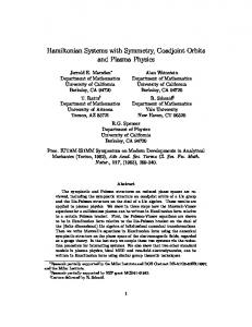
As an example of the methods described in the previous section, we consider the iteration on C2 which has O(2) symmetry given by z1n+1 = (α + β1 |z1n |2 + γ1 Re(z1n z¯2n ))z1n + δ1 z2n z2n+1 = (λ + β2 |z2n |2 + γ2 Re(z1n z¯2n ))z2n + δ2 z1n , where α = −2.6, β1 = 1.5, β2 = 0.4, γ1 = 0.7, γ2 = 0.5, δ1 = −0.5 and δ2 = 0.3 (see [1, 4]). The parameter λ will be used as the perturbation parameter. These equations can be written in terms of the invariant coordinates R2 , C and S as R2n+1 = δ22 R1n + 2δ2 (λ + β2 R2n + γ2 C n )C n + (λ + β2 R2n + γ2 C n )2 R2n C n+1 = (α + β1 R1n + γ1 C n )δ2 R1n + δ1 (λ + β2 R2n + γ2 C n )R2n +((α + β1 R1n + γ1 C n )(λ + β2 R2n + γ2 C n ) + δ1 δ2 )C n S n+1 = S n [(α + β1 R1n + γ1 C n )(λ + β2 R2n + γ2 C n ) − δ1 δ2 ] where R1 = (C 2 + S 2 )/R2 . When λ = −0.48, the map behaves chaotically and the chaotic attractor is shown in Fig. 1. The projection of the chaotic motion onto the two-dimensional symmetric subspace of the orbit space is shown in Fig. 2. Note that 5
y1
1.5
1.5
1.0
1.0
0.5
0.5 y2
0.0
0.0
-0.5
-0.5
-1.0
-1.0
-1.5 -1.5
-1.0
-0.5
0.0 x1
0.5
1.0
-1.5 -1.5
1.5
-1.0
-0.5
0.0 x2
0.5
1.0
1.5
Figure 1: The chaotic attractor at λ = −0.48.
-0.4
-0.6
C
-0.8
-1.0
-1.2 0.2
0.4
0.6
0.8
1.0
1.2
R2
Figure 2: The chaotic attractor projected onto the symmetric subspace of the orbit space. • = period 2 points in the symmetric subspace.
6
y1
1.5
1.5
1.0
1.0
0.5
0.5 y2
0.0
0.0
-0.5
-0.5
-1.0
-1.0
-1.5 -1.5
-1.0
-0.5
0.0 x1
0.5
1.0
-1.5 -1.5
1.5
-1.0
-0.5
0.0 x2
0.5
1.0
1.5
Figure 3: The controlled orbit at λ = −0.48. • = controlled period 2 points. the chaotic attractor is well away from the origin in both the z1 and z2 planes and so there is no problem is fixing the coordinate R2 as one of the variables in the orbit space map. The chaotic attractor shown in Figs. 1 and 2 contains a period 2 orbit with S = 0. The period 2 points occur in orbit space coordinates at R2 = 0.71183, C = −0.64032 and at R2 = 0.43897, C = −0.81882. The eigenvalues of the linearisation of the twice iterated orbit space map evaluated at the first of these period 2 points are 0.31524, −2.6148 and 0.99475. The eigenvalue associated with perturbations in the normal direction is 0.99475 and so the period 2 points are just stable in this direction. Thus, the two-dimensional system (3.2) in the symmetric subspace can be used to determine the parameter perturbations. The two-dimensional vector of derivatives with respect to the parameter λ evaluated at the period 2 point is given by w=
"
−2.2171 1.4023
#
.
Using all this information, the control method was implemented in this system. The iterates after control has been applied are shown in Fig. 3. Note that there is a slow drift round the group orbit before the iteration finally settles down onto the period 2 points at one point on the group orbit. This is related to the eigenvalue which is very close to 1 which implies that the contraction in S is very slow. We also note from (2.2) that for small S, the drift is approximately proportional to S and this is why it takes a long time for the drift to slow down. Clearly, if the third eigenvalue was smaller, then the drift along the group orbit during the control phase would be much smaller also. As the parameter λ is decreased from −0.48, the symmetric period 2 points which were used for control undergo a symmetry-breaking bifurcation giving rise to nonsymmetric period 2 orbits. For example, taking λ = −0.5, we obtain period 2 points in 7
y1
1.5
1.5
1.0
1.0
0.5
0.5 y2
0.0
0.0
-0.5
-0.5
-1.0
-1.0
-1.5 -1.5
-1.0
-0.5
0.0 x1
0.5
1.0
-1.5 -1.5
1.5
-1.0
-0.5
0.0 x2
0.5
1.0
1.5
Figure 4: The controlled orbit at λ = −0.5. orbit space coordinates at R2 = 0.70911, C = −0.61403, S = 0.15290 and R2 = 0.43787, C = −0.79357, S = 0.19768. The eigenvalues of the linearisation of the twice iterated map evaluated at the first of these period 2 points are −2.6369, 0.37342 and 0.86954. Clearly the unstable manifold has dimension one and so it is possible to stabilise such a period 2 orbit using only one parameter. The vector of derivatives with respect to the parameter λ evaluated at the period 2 point is given by
−2.16722 w = 1.26733 . −0.53576 The control method was implemented at this new parameter value. Since S 6= 0, the corresponding stabilised orbit in the original coordinates is a drifting period 2 orbit. The stabilised orbit is shown in Fig. 4.
5
Applications
This method is applicable to Poincar´e maps which arise from periodically forced differential equations. Since the Poincar´e map inherits the symmetry properties of the differential equations, it is appropriate for a forced system which has O(2) symmetry. In this context, fixed points of the Poincar´e map correspond to periodic orbits of the differential equations while drifting fixed points correspond to quasi-periodic solutions. One example of such a system is the vertically forced spherical pendulum. This is a four-dimensional system of differential equations which gives rise to a four-dimensional Poincar´e map with O(2) symmetry. However, in this case there are no orbits which drift along group orbits. This can be shown by considering the normal derivative to the two-dimensional symmetric subspace which is always negative. The vertically forced 8
double spherical pendulum does have orbits which drift along the group orbit and so these methods could be applied in this context. The equations are now eight-dimensional giving rise to an eight-dimensional Poincar´e map with O(2) symmetry.
References [1] Aston, P.J., Bifurcation and chaos in iterated maps with O(2) symmetry, Int. J. Bif. Chaos 5, 701-724, 1995. [2] Aston, P.J. and Bird, C.M., Synchronisation of coupled systems via parameter perturbations. To appear in Phys. Rev. E. [3] Bird, C.M., The Control of Chaos, PhD Thesis, University of Surrey, 1996. [4] Dellnitz, M., Golubitsky, M. and Melbourne, I., Mechanisms of symmetry creation. In Bifurcation and Symmetry, ISNM 104, Eds. E. Allgower, K. B¨ohmer and M. Golubitsky, Birkh¨auser, 99-109, 1992. [5] Marsden, J.E., Lectures on Mechanics, LMS Lecture Note Series 174, CUP, 1992. [6] Ott, E., Grebogi, C. and Yorke, J.A., Controlling chaos, Phys. Rev. Lett. 64, 11961199, 1990. [7] Shinbrot, T., Grebogi, C., Ott, E. and Yorke, J.A., Using small perturbations to control chaos, Nature 363, 411-417, 1993.
9