Controlling Generalization and Polyvariance in Partial ... - CiteSeerX

Controlling Generalization and Polyvariance in Partial Deduction of Normal Logic Programs MICHAEL LEUSCHEL, BERN MARTENS, and DANNY DE SCHREYE Katholieke Universiteit Leuven

Given a program and some input data, partial deduction computes a specialized program handling any remaining input more efficiently. However, controlling the process well is a rather difficult problem. In this article, we elaborate global control for partial deduction: for which atoms, among possibly infinitely many, should specialized relations be produced, meanwhile guaranteeing correctness as well as termination? Our work is based on two ingredients. First, we use the concept of a characteristic tree, encapsulating specialization behavior rather than syntactic structure, to guide generalization and polyvariance, and we show how this can be done in a correct and elegant way. Second, we structure combinations of atoms and associated characteristic trees in global trees registering “causal” relationships among such pairs. This allows us to spot looming nontermination and perform proper generalization in order to avert the danger, without having to impose a depth bound on characteristic trees. The practical relevance and benefits of the work are illustrated through extensive experiments. Finally, a similar approach may improve upon current (on-line) control strategies for program transformation in general such as (positive) supercompilation of functional programs. It also seems valuable in the context of abstract interpretation to handle infinite domains of infinite height with more precision. Categories and Subject Descriptors: D.1.2 [Programming Techniques]: Automatic Programming; I.2.3 [Artificial Intelligence]: Deduction and Theorem Proving—logic programming; D.1.6 [Programming Techniques]: Logic Programming; F.4.1 [Mathematical Logic and Formal Languages]: Mathematical Logic—logic programming; I.2.2 [Artificial Intelligence]: Automatic Programming General Terms: Algorithms, Performance, Theory Additional Key Words and Phrases: Flow analysis, partial deduction, partial evaluation, program transformation, supercompilation

Michael Leuschel is Postdoctoral Fellow of the Fund for Scientific Research - Flanders (Belgium) (F.W.O.), and was also supported by the Belgian GOA “Non-Standard Applications of Abstract Interpretation.” Bern Martens is a Postdoctoral Fellow of the K.U.Leuven Research Council, Belgium, and was also partially supported by the HCM Network “Logic Program Synthesis and Transformation,” contract no. CHRX-CT-93-00414, University of Padova, Italy, and the Belgian GOA “Non-Standard Applications of Abstract Interpretation.” Danny De Schreye is Senior Research Associate of the Fund for Scientific Research - Flanders (Belgium) (F.W.O.). Authors’ addresses: Departement Computerwetenschappen, K.U. Leuven, Celestijnenlaan 200A, B-3001 Heverlee, Belgium; email: {michael; bern; dannyd}@cs.kuleuven.ac.be Permission to make digital/hard copy of all or part of this material without fee for personal or classroom use provided that the copies are not made or distributed for profit or commercial advantage, the ACM copyright/server notice, the title of the publication, and its date appear, and notice is given that copying is by permission of the ACM, Inc. To copy otherwise, to republish, to post on servers, or to redistribute to lists requires prior specific permission and/or a fee. c 1998 ACM 0164-0925/98/0100-0208 $5.00

ACM Transactions on Programming Languages and Systems, Vol. 20, No. 1, January 1998, Pages 208–258.

Controlling Generalization and Polyvariance

·

209

1. INTRODUCTION A major concern in the specialization of functional (e.g., see Consel and Danvy [1993], Jones et al. [1993], and Turchin [1986]) as well as logic programs (e.g., see Lloyd and Shepherdson [1991], Komorowski [1992], Gallagher [1993], Pettorosii and Prooietti [1994], and De Schreye et al. [1995]) has been the issue of control: how can the transformation process be guided in such a way that termination is guaranteed and results are satisfactory? This problem has been tackled from two (until now) largely separate angles: the so-called off-line versus on-line approaches. Partial evaluation of functional programs [Consel and Danvy 1993; Jones et al. 1993] has mainly stressed the former, while supercompilation of functional programs [Turchin 1986; 1988; Søensen and Gl¨ uck 1995] and partial deduction of logic programs [Bol 1993; Bruynooghe et al. 1992; Gallagher and Bruynooghe 1991; Martens and De Schreye 1996 Martens and Gallagher 1995; Sahlin 1993] have concentrated on on-line control. (Some exceptions are the works of Weise et al. [1991], Mogensen and Bondorf [1992], Leuschel [1994], Jørgensen and Leuschel [1996], and Bruynooghe et al. [1998].) The concrete setting of the present article concerns logic program partial deduction. We are, however, convinced that its contribution is not limited to that particular field. Indeed, its techniques and ideas are also relevant to the control of supercompilation and on-line partial evaluation of functional (and perhaps also imperative) languages. Moreover, even abstract interpretation can benefit from them. We return to these points in Section 4.7. In partial deduction of logic programs, one distinguishes two levels of control [Gallagher 1993; Martens and Gallagher 1995]: the local and the global level. In a nutshell, the local level decides on how SLD(NF)-trees for individual atoms should be built. The (branches of the) resulting trees allow us to construct specialized clauses for the given atoms [Benkerimi and Lloyd 1990; Lloyd and Shepherdson 1991]. At the global level on the other hand, one typically attends to the overall correctness of the resulting program (satisfying the closedness condition in Lloyd and Shepherdson [1991]) and strives to achieve the “right” amount of polyvariance, producing sufficiently many (but not more) specialized versions for each predicate definition in the original program. At both levels, in the context of providing a fully automatic tool, termination is obviously of prime importance. In this article, it is to the global level that we turn our attention. The concept of characteristic trees has been proposed as a basis for the global control of partial deduction in Gallagher and Bruynooghe [1991] and Gallagher [1991]. The main idea is, instead of using the syntactic structure to decide upon polyvariance, to examine the specialization behavior of the atoms to be specialized: only if this behavior is sufficiently different from one atom to the other should different specialized versions be generated. However, the approaches based on characteristic trees have been, up to now, ridden by two major problems. First, they failed to preserve the characteristic trees upon generalization: two atoms with identical specialization behavior may be generalized by one with a completely different specialization behavior. This may lead to significant losses in specialization, as well as to problems for the termination of the partial deduction process. Second, the characteristic trees have always been limited by some ad hoc depth bound, possibly leading to very undesirable specialization results (as we will show later in the article). ACM Transactions on Programming Languages and Systems, Vol. 20, No. 1, January 1998.

210

·

M. Leuschel et al.

In the present article, we solve these two problems. After presenting some required background about partial deduction and characteristic trees in Section 2, we address the first problem in Section 3 by developing the ecological partial deduction principle, ensuring the preservation of characteristic trees. In Section 4 we then solve the second problem, blending the general framework in Martens and Gallagher [1995] with the framework developed in Section 3. We thus obtain an elegant, sophisticated, and precise apparatus for on-line global control of partial deduction. Benchmark results can be found in Section 5. Section 6 subsequently concludes the article. Finally, we would like to mention that two workshop papers address part of the material in a preliminary form: —Leuschel [1995] describes how to impose characteristic trees and perform setbased partial deduction with characteristic atoms, —while Leuschel and Martens [1996] elaborates the former approach into one using global trees, and thus not requiring any depth bound. 2. PRELIMINARIES AND MOTIVATIONS Throughout this article, we suppose familiarity with basic notions in logic programming [Lloyd 1987] and partial deduction [Lloyd and Shepherdson 1991]. Notational conventions are standard and self-evident. In particular, in programs, we denote variables through (strings starting with) an uppercase symbol, while the notations of constants, functions, and predicates begin with a lowercase character. Unless stated explicitly otherwise, the terms “(logic) program” and “goal” will refer to a normal logic program and goal, respectively. By an expression we mean either a term, an atom, a literal, a conjunction, a disjunction, or a program clause. Expressions are constructed using the language LP which we implicitly assume underlying the program P under consideration. LP may contain additional symbols not occurring in P , but, unless explicitly stated otherwise, LP contains only finitely many constant, function, and predicate symbols. To simplify the presentation we also assume that, when talking about expressions, predicate symbols and connectives are treated like functors which cannot be confounded with the original functors and constants (e.g., ∧ and ← are binary functors distinct from the other binary functors). As common in partial deduction, the notion of SLDNF-trees is extended to allow incomplete SLDNF-trees which may contain leaves where no literal has been selected for a further derivation step. Leaves of the latter kind will be called dangling [Martens and De Schreye 1996]. 2.1 Partial Deduction In contrast to (full) evaluation, a partial evaluator is given a program P along with a part of its input, called the static input. The remaining part of the input, called the dynamic input, will only be known or given at some later point in time. Given the static input S, the partial evaluator then produces a specialized version PS of P which, when given the dynamic input D, produces the same output as the original program P . In the context of logic programming, full input to a program P consists of a goal G, and evaluation corresponds to constructing a complete SLDNF-tree for P ∪ {G}. ACM Transactions on Programming Languages and Systems, Vol. 20, No. 1, January 1998.


·

211

Partial input then takes the form of a partially instantiated goal G′ . One often uses the term partial deduction to refer to partial evaluation of pure logic programs (see Komorowski [1992]), a convention we will adhere to in this article. So, given this goal G′ and the original program P , partial deduction produces a new program P ′ which is P “specialized” to the goal G′ : P ′ can be called for all instances of G′ , producing the same output as P , but often much more efficiently. In order to avoid constructing infinite SLDNF-trees for partially instantiated goals, partial deduction is based on constructing finite, but possibly incomplete SLDNF-trees for a set of atoms A. The derivation steps in these SLDNF-trees correspond to the computation steps performed (beforehand) by the partial deducer , and the specialized program is extracted from these trees by constructing one specialized clause per branch. The incomplete SLDNF-trees are obtained by applying an unfolding rule, defined as follows: Definition 2.1.1. An unfolding rule U is a function which, given a program P and a goal G, returns a finite and possibly incomplete SLDNF-tree for P ∪ {G}. For reasons to be clarified later, Definition 2.1.1 is so general as to even allow a trivial SLDNF-tree, i.e., one whose root is a dangling leaf. Specialized clauses are extracted from the SLDNF-trees as follows: Definition 2.1.2. Let P be a program and A an atom. Let τ be a finite, incomplete, and nontrivial1 SLDNF-tree for P ∪{← A}. Let ← G1 , . . . , ← Gn be the goals in the (nonroot) leaves of the nonfailing branches of τ . Let θ1 , . . . , θn be the computed answers of the derivations from ← A to ← G1 , . . . , ← Gn respectively. Then the set of resultants resultants(τ ) is defined to be {Aθ1 ← G1 , . . . , Aθn ← Gn }. Partial deduction, as defined for example by Lloyd and Shepherdson [1991] and Benkerimi and Lloyd [1990], uses the resultants for a given set of atoms A to construct the specialized program and for each atom in A a different specialized predicate definition is generated, replacing the original definition in P . Under the conditions stated in Lloyd and Shepherdson [1991], namely closedness and independence, correctness of the specialized program is guaranteed. Independence requires that no two atoms in A have a common instance. This ensures that no two specialized predicate definitions match the same (run-time) call. Usually this condition is satisfied by performing a renaming of the atoms in A (see Gallagher and Bruynooghe [1990] and Benkerimi and Hill [1993]). Closedness (as well as the related notion of coveredness in Benkerimi and Lloyd [1990]) basically requires that every atom in the body of a resultant is matched by a specialized predicate definition. This guarantees that A forms a complete description of all possible computations that can occur at run-time of the specialized program. The main practical difficulty of partial deduction is the control of polyvariance problem, which reduces to finding a terminating procedure to produce a finite set of atoms A which satisfies the above correctness conditions while at the same time providing as much potential for specialization as possible.

1 To

avoid the problematic resultant A ← A. ACM Transactions on Programming Languages and Systems, Vol. 20, No. 1, January 1998.

212

·

M. Leuschel et al.

2.2 Abstraction Termination is usually obtained by using a suitable abstraction operator, defined as follows: Definition 2.2.1. Let A and A′ be sets of atoms. Then A′ is an abstraction of A if and only if every atom in A is an instance of an atom in A′ . An abstraction operator is an operator which maps every finite set of atoms to a finite abstraction of it. The following generic scheme, based on a similar one in Gallagher [1991] and Gallagher [1993], describes the basic layout of practically all algorithms for controlling partial deduction. Algorithm 2.2.2 (Standard Partial Deduction). Input: A program P and a goal G Output: A specialized program P ′ Initialization: i = 0 , Ai = {A | A is an atom in G } repeat for each Ak ∈ Ai , compute a finite SLDNF-tree τk for P ∪ {← Ak } by applying unfolding rule U ; let A′i := Ai ∪ {Bl |Bl is an atom in a leaf of some tree τk , such that Bl is not an instance 2 of any Aj ∈ Ai } ; let Ai+1 := abstract(A′i ) where abstract is an abstraction operator let i := i + 1; until Ai+1 = Ai Apply a renaming transformation to Ai to ensure independence and then construct P ′ by taking resultants. In itself the use of an abstraction operator does not yet guarantee global termination. But if the above algorithm terminates then independence and coveredness are ensured. With this observation we can reformulate the control of polyvariance problem as one of finding an abstraction operator which maximizes specialization while ensuring termination. The abstraction operator examines the set of atoms to be partially deduced and then decides which atoms should be abstracted and which ones should be left unmodified. A very simple abstraction operator, which ensures termination, can be obtained by imposing a finite maximum number of atoms in Ai and using the most specific generalization (msg)3 to stick to that maximum. This approach is however unsatisfactory. First, it involves an ad hoc maximum number, which might lead to either too much or too little polyvariance, depending on the context. Second, the msg is just based on the syntactic structure of the atoms to be specialized. This is generally not such a good idea. Indeed, two atoms can be unfolded and specialized in a very similar way in the context of one program P1 , while in the context of another program P2 their specialization behavior can be drastically different. The 2 One 3 Also

can also use the variant test to make the algorithm more precise. known as antiunification or least general generalization; see for instance Lassez et al. [1988].

ACM Transactions on Programming Languages and Systems, Vol. 20, No. 1, January 1998.

Controlling Generalization and Polyvariance ← append ([a], X, Y )

@ (2) @ R @ ← append ([], X, Y ′ )

·

213

← append (X, [a], Y ) (1)

2

@ (2) @ R @ ← append (X ′ , [a], Y ′ )

(1)

2 Fig. 1.

SLD-trees τB and τC for Example 2.2.3.

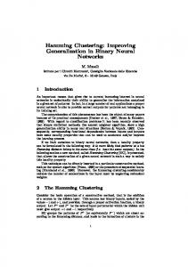
syntactic structure of the two atoms is of course unaffected by the particular context, and an operator like the msg will perform exactly the same abstraction within P1 and P2 , although different generalizations might be called for. A better candidate for an abstraction might be to examine the SLDNF-trees generated for these atoms. These trees capture (to some depth) how the atoms behave computationally in the context of the respective programs. They also capture (part of) the specialization that has been performed on these atoms. An abstraction operator which takes these trees into account will notice their similar behavior in the context of P1 and their dissimilar behavior within P2 , and can therefore take appropriate actions in the form of different generalizations. The following example illustrates these points. Example 2.2.3. Let P be the append program: (1) append ([], Z, Z) ← (2) append ([H|X], Y, [H|Z]) ← append (X, Y, Z) Note that we have added clause numbers, which we will henceforth take the liberty to incorporate into illustrations of SLD-trees in order to clarify which clauses have been resolved with. To avoid cluttering the figures we will also sometimes drop the substitutions in such figures. Let A = {B, C} be a dependent set of atoms, where B = append ([a], X, Y ) and C = append (X, [a], Y ). Typically a partial deducer will unfold the two atoms of A in the way depicted in Figure 1, returning the finite SLD-trees τB and τC . These two trees, as well as the associated resultants, have a very different structure. The atom append ([a], X, Y ) has been fully unfolded, and we obtain for resultants(τB ) the single fact append ([a], X, [a|X]) ← while for append (X, [a], Y ) we obtain for resultants(τC ) the following set of clauses: append ([], [a], [a]) ← append ([H|X], [a], [H|Z]) ← append (X, [a], Z) So, in this case, it is vital to keep separate specialized versions for B and C and not abstract them for example by their msg. However, it is very easy to come up with another context in which the specialization behaviors of B and C are almost indiscernible. Take for instance the following ACM Transactions on Programming Languages and Systems, Vol. 20, No. 1, January 1998.

214

·

M. Leuschel et al. ← append ∗ ([a], X, Y ) (1∗ )

2

@ (2∗ ) @ R @ ← append ∗ ([], TX , E)

← append ∗ (X, [a], Y ) (1∗ )

2

@ (2∗ ) @ R @ ← append ∗ (TX , [], E)

fail

Fig. 2.

fail

∗ and τ ∗ for Example 2.2.3. SLD-trees τB C

program P ∗ in which append ∗ no longer appends two lists, but finds common elements at common positions: (1∗ ) append ∗ ([X|TX ], [X|TY ], [X]) ← (2∗ ) append ∗ ([X|TX ], [Y |TY ], E) ← append ∗ (TX , TY , E) The associated finite SLD-trees τB∗ and τC∗ , depicted in Figure 2, are now almost fully identical. In that case, it is not useful to keep different specialized versions for B and C because the following single set of specialized clauses could be used for B and C without specialization loss: append ∗ ([a|T1 ], [a|T2 ], [a]) ← This illustrates that the syntactic structures of B and C alone provide insufficient information for a satisfactory control of polyvariance and that a refined abstraction operator should also take the associated SLDNF-trees into consideration. 2.3 Characteristic Paths and Trees Above we have illustrated the interest of examining the SLDNF-trees generated for the atoms to be partially deduced and for example only abstract atoms if their associated trees are “similar enough.” A crucial question is of course which part of these SLDNF-trees should be taken into account to decide upon similarity. If we take everything into account, i.e., only abstract two atoms if their associated trees are identical, this amounts to performing no abstraction at all. So an abstraction operator should focus on the “essential” structure of an SLDNF-tree and for instance disregard the particular substitutions and goals within the tree. The following two definitions, adapted from Gallagher [1991], do just that: they characterize the essential structure of SLDNF-derivations and trees. Definition 2.3.1 (Characteristic Path). Let G0 be a goal, and let P be a normal program whose clauses are numbered. Let G0 , . . . , Gn be the goals of a finite, possibly incomplete SLDNF-derivation D of P ∪ {G0 }. The characteristic path of the derivation D is the sequence hl0 : c0 , . . . , ln−1 : cn−1 i, where li is the position of the selected literal in Gi , and ci is defined as follows: —if the selected literal is an atom, then ci is the number of the clause chosen to resolve with Gi . —if the selected literal is ¬p(t¯), then ci is the predicate p. ACM Transactions on Programming Languages and Systems, Vol. 20, No. 1, January 1998.


·

215

The set containing the characteristic paths of all possible finite SLDNF-derivations for P ∪ {G0 } will be denoted by chpaths(P, G0 ). For example, the characteristic path of the derivation associated with the only branch of the SLD-tree τB in Figure 1 is h1 : 2, 1 : 1i. Recall that an SLDNF-derivation D can be either failed, incomplete, successful, or infinite. As we will see below, characteristic paths will only be used to characterize finite and nonfailing derivations of atomic goals. Once the top-level goal is known, the characteristic path is sufficient to reconstruct all the intermediate goals as well as the final one. So, using p in the second point of Definition 2.3.1 instead of a unique symbol to signal the selection of a negative literal is a matter of convention rather than necessity. Now that we have characterized derivations, we can characterize goals through the derivations in their associated SLDNF-trees. Definition 2.3.2 (Characteristic Tree). Let G be a goal, P a normal program, and τ a finite SLDNF-tree for P ∪{G}. Then the characteristic tree τˆ of τ is the set containing the characteristic paths of the nonfailing SLDNF-derivations associated with the branches of τ . τˆ is called a characteristic tree if and only if it is the characteristic tree of some finite SLDNF-tree. Let U be an unfolding rule such that U (P, G) = τ . Then τˆ is also called the characteristic tree of G (in P ) via U . We introduce the notation chtree(G, P, U ) = τˆ. We also say that τˆ is a characteristic tree of G (in P ) if it is the characteristic tree of G (in P ) via some unfolding rule U . Note that the characteristic path of an empty derivation is the empty path hi, and the characteristic tree of a trivial SLDNF-tree is {hi}. Although a characteristic tree only contains a collection of characteristic paths, the actual tree structure is not lost and can be reconstructed without ambiguity. The “glue” is provided by the clause numbers inside the characteristic paths (branching in the tree is indicated by differing clause numbers). Example 2.3.3. The characteristic trees of the finite SLD-trees τB and τC in Figure 1 are {h1 : 2, 1 : 1i} and {h1 : 1i, h1 : 2i} respectively. The characteristic trees of the finite SLD-trees τB∗ and τC∗ in Figure 2 are both {h1 : 1∗ i}. The characteristic tree captures all the relevant aspects of specialization, attained by the local control for a particular atom: —The branches that have been pruned through the unfolding process (namely those that are absent from the characteristic tree). —How deep ← A has been unfolded and which literals and clauses have been resolved with each other in that process. This captures the computation steps that have already been performed at partial deduction time. —The number of clauses in the resultants of A (namely one per characteristic path) and (implicitly) which predicates are called in the bodies of the resultants. As we will see later, this means that a single predicate definition can (in principle) be used for two atoms which have the same characteristic tree. ACM Transactions on Programming Languages and Systems, Vol. 20, No. 1, January 1998.

216

·

M. Leuschel et al. ← member (a, [a]) (1)

2

← member (a, [a, b])

@ (2) @ R @

← member (a, [])

(1)

2

@ (2) @ R @

← member (a, [b]) (2)

fail

?

← member (a, []) fail Fig. 3.

SLD-trees for Example 2.3.4.

A specialization aspect that does not materialize within a characteristic tree is how the atoms in the leaves of the associated SLDNF-tree are further specialized, i.e., the global control and precision are not captured. By examining only the nonfailing branches we do not capture how exactly some branches were pruned. The following example illustrates why this is adequate and even beneficial. Example 2.3.4. Let P be the following program: (1) member (X, [X|T ]) ← (2) member (X, [Y |T ]) ← member (X, T ) Let A = member (a, [a, b]) and B = member (a, [a]). Suppose that A and B are unfolded as depicted in Figure 3. Then both these atoms have the same characteristic tree τ = {h1 : 1i} although the associated SLDNF-trees differ by the structure of their failing branches. However, this is of no relevance, because the failing branches do not materialize within the resultants (i.e., the specialized code generated for the atoms), and furthermore the single resultant member (a, [a|T ]) ← could be used for both A and B without loosing any specialization. In summary, characteristic trees seem to be an almost ideal vehicle for a refined control of polyvariance, a fact we will try to exploit in the following. 2.4 An Abstraction Operator Using Characteristic Trees The following abstraction operator represents a first attempt at using characteristic trees for the control of polyvariance. Basically it classifies atoms according to their associated characteristic tree. Generalization, in this case the msg, is then only applied on those atoms which have the same characteristic tree. Definition 2.4.1 (chabs P,U ). Let P be a normal program, U an unfolding rule and A a set of atoms. For every characteristic tree τ , let Aτ be defined as Aτ = {A | A ∈ A ∧ chtree(← A, P, U ) = τ }. The abstraction operator chabs P,U is then defined as chabs P,U (A) = {msg(Aτ ) | τ is a characteristic tree}. Unfortunately, although for a lot of practical cases chabsP,U performs quite well, it does not always preserve the characteristic trees, entailing a sometimes quite severe loss of precision and specialization. We first illustrate the possible specialization losses in the following example. ACM Transactions on Programming Languages and Systems, Vol. 20, No. 1, January 1998.


·

217

Example 2.4.2. Let us return to Example 2.3.4 and specialize the member program for A = member (a, [a, b]) and B = member (a, [a]). First we put the atoms into A0 : A0 = {member (a, [a, b]), member (a, [a])}. For both atoms the associated characteristic tree is τ = {h1 : 1i}, given for example a determinate unfolding rule with lookahead (see Figure 3). Thus chabs P,U , as well as the method of Gallagher [1991], abstracts the two atoms and produces the generalized set A1 = {member (a, [a|T ])}. Unfortunately, the generalized atom member (a, [a|T ]) has a different characteristic tree τ ′ , independently of the particular unfolding rule. For a determinate unfolding rule with lookahead we obtain τ ′ = {h1 : 1i, h1 : 2i}. This loss of precision leads to suboptimal specialized programs. At the next step of the algorithm the atom member (a, T ) will be added to A1 . This atom also has the characteristic tree τ ′ under U . Hence the final set A2 equals {member(a, L)} (containing the msg of member (a, [a|T ]) and member (a, T )}), and we obtain the following specialization, suboptimal for ← member (a, [a, b]), member (a, [a]): (1’) member (a, [a|T ]) ← (2’) member (a, [X|T ]) ← member (a, T ) So, although partial deduction was able to figure out that member (a, [a, b]) as well as member (a, [a]) have only one nonfailing resolvent, this information has been lost due to an imprecision of the abstraction operator, thereby leading to a suboptimal residual program in which the determinacy is not explicit (and redundant computation steps occur at run-time). Note that a “perfect” program for ← member (a, [a, b]), member (a, [a]) would just consist of (a filtered version of) clause (1’). As explained by Leuschel and De Schreye [1998], these losses of precision can also lead to nontermination of the partial deduction process, further illustrating the importance of preserving characteristic trees upon generalization. 3. PARTIAL DEDUCTION WITH CHARACTERISTIC ATOMS We now present a way to preserve characteristic trees during abstraction. The basic idea is to simply impose characteristic trees on the generalized atoms. 3.1 Characteristic Atoms We first introduce the crucial notion of a characteristic atom. Definition 3.1.1. A characteristic atom is a couple (A, τ ) consisting of an atom A and a characteristic tree τ . Note that τ is not required to be a characteristic tree of A in the context of the particular program P under consideration. Example 3.1.2. Let τ = {h1 : 1i} be a characteristic tree. Then the couples CA1 = (member (a, [a, b]), τ ) and CA2 = (member (a, [a]), τ ) are characteristic atoms. CA3 = (member (a, [a|T ]), τ ) is also a characteristic atom, but for example in the context of the member program P from Example 2.3.4, τ is not a characteristic tree of its atom component member (a, [a|T ]) (cf. Example 2.4.2). Intuitively, such a situation corresponds to imposing the characteristic tree τ on the atom member (a, [a|T ]). Indeed, as we will see later, CA3 can be seen as a precise ACM Transactions on Programming Languages and Systems, Vol. 20, No. 1, January 1998.

218

·

M. Leuschel et al.

generalization (in P ) of the atoms member (a, [a, b]) and member (a, [a]), solving the problem of Example 2.4.2. A characteristic atom will be used to represent a possibly infinite set of atoms, called its concretizations. This is nothing really new: in standard partial deduction, an atom A also represents a possibly infinite set of concrete atoms, namely its instances. The characteristic tree component of a characteristic atom will just act as a constraint on the instances, i.e., keeping only those instances which have a particular characteristic tree. This is captured by the following definition. Definition 3.1.3 (Concretization). Let (A, τA ) be a characteristic atom and P a program. An atom B is a precise concretization of (A, τA ) (in P )4 if and only if B is an instance of A and, for some unfolding rule U , chtree(← B, P, U ) = τA . An atom is a concretization of (A, τA ) (in P ) if and only if it is an instance of a precise concretization of (A, τA ) (in P ). We denote the set of concretizations of (A, τA ) in P by γP (A, τA ). A characteristic atom with a nonempty set of concretizations in P will be called well-formed in P or a P -characteristic atom. We will from now on usually restrict our attention to P -characteristic atoms. In particular, the partial deduction algorithm presented later on in Section 3.4 will only produce P -characteristic atoms, where P is the original program to be specialized. Example 3.1.4. Take the characteristic atom CA3 = (member (a, [a|T ]), τ ) with τ = {h1 : 1i} from Example 3.1.2 and the member program P from Example 2.3.4. The atoms member (a, [a]) and member (a, [a, b]) are precise concretizations of CA3 in P (see Figure 3). Also, neither member (a, [a|T ]) nor member (a, [a, a]) are concretizations of CA3 in P . Finally, observe that CA3 is a P -characteristic atom while for instance (member (a, [a|T ]), {h2 : 5i} or even (member (a, [a|T ]), {h1 : 2i} are not. Example 3.1.5. Let P be the following simple program: (1) p(a, Y ) ← (2) p(X, Y ) ← ¬q(Y ), q(X) (3) q(b) ← Let τ = {h1 : 1i, h1 : 2, 1 : q, 1 : 3i} and CA = (p(X, Y ), τ ). Then p(X, a) and p(X, c) are precise concretizations of CA in P and neither p(b, b), p(X, b), p(a, Y ), nor p(X, Y ) are concretizations of CA in P . Also p(b, a) and p(a, a) are both concretizations of CA in P , but they are not precise concretizations. Observe that the selection of the negative literal ¬q(Y ), corresponding to 1 : q in τ , is unsafe for ← p(X, Y ), but that for any concretization of CA in P the corresponding derivation step is safe and succeeds (i.e., the negated atom is ground and fails finitely). Note that by definition the set of concretizations associated with a characteristic atom is downward closed (or closed under substitution).This observation justifies the following definition. 4 If

P is clear from the context, we will not explicitly mention it.



·

219

Definition 3.1.6 (Unconstrained Characteristic Atom). A P -characteristic atom (A, τA ) with A ∈ γP (A, τA ) is called unconstrained (in P ). The concretizations of an unconstrained characteristic atom (A, τA ) are identical to the instances of the ordinary atom A (because the concretizations are downward closed, and γP (A, τ ) contains no atom strictly more general than A). So, characteristic atoms along with Definition 3.1.3 provide a proper generalization of the way atoms are used in the standard partial deduction approach. 3.2 Generating Resultants We now address the generation of resultants for characteristic atoms. We need the following definition in order to formalize the resultants associated with a characteristic atom. Definition 3.2.1. A generalized SLDNF-derivation is either composed of ordinary SLDNF-derivation steps or of derivation steps in which a nonground negative literal is selected and removed. Generalized SLDNF-derivations will be called unsafe if they contain steps of the latter kind and safe if they do not. Most of the definitions for ordinary SLDNF-derivations, like the associated characteristic path and resultant, carry over to generalized derivations. We first define a set of possibly unsafe generalized SLDNF-derivations associated with a characteristic atom: Definition 3.2.2 (DP (A, τ )). Let P be a program and (A, τ ) a P -characteristic atom. If τ 6= {hi} then DP (A, τ ) is the set of all generalized SLDNF-derivations of P ∪ {← A} such that their characteristic paths are in τ . If τ = {hi} then DP (A, τ ) is the set of all nonfailing SLD-derivations of P ∪ {← A} of length 1.5 Note that the derivations in DP (A, τ ) are necessarily finite and nonfailing (because (A, τ ) is a P -characteristic atom; see also Lemma B.2.9, in the electronic appendix to this article). We will call a P -characteristic atom (A, τ ) safe (in P ) if and only if all derivations in DP (A, τ ) are safe. An unconstrained characteristic atom in P is safe in P .6 Using the definition of DP (A, τ ), we can now define the resultants, and hence the partial deduction, associated with characteristic atoms: Definition 3.2.3 (Partial Deduction of (A, τ )). Let P be a program and (A, τ ) a P -characteristic atom. Let {D1 , . . . , Dn } be the generalized SLDNF-derivations in DP (A, τ ), and let ← G1 , . . . , ← Gn be the goals in the leaves of these derivations. Let θ1 , . . . , θn be the computed answers of the derivations from ← A to ← G1 , . . . , ← Gn respectively. Then the set of resultants {Aθ1 ← G1 , . . . , Aθn ← Gn } is called the partial deduction of (A, τ ) in P . Every atom occurring in some of the Gi will be called a leaf atom (in P ) of (A, τ ). We will denote the set of such leaf atoms by leavesP (A, τ ). 5 Just

like in ordinary partial deduction, we want to construct only nontrivial SLDNF-trees for P ∪ {← A} to avoid the problematic resultant A ← A. 6 Because A must be a precise concretization of (A, τ ), we have that τ is a characteristic tree of A, and thus all derivations in DP (A, τ ) are ordinary SLDNF-derivations and therefore safe. ACM Transactions on Programming Languages and Systems, Vol. 20, No. 1, January 1998.

220

·

M. Leuschel et al.

Example 3.2.4. The partial deduction of (member (a, [a|T ]), {h1 : 1i}) in the program P of Example 2.3.4 is {member(a, [a|T ]) ←}. Note that it is different from any set of resultants that can be obtained for the ordinary atom member (a, [a|T ]). However, as we will prove below, the partial deduction is correct for any concretization of (member (a, [a|T ]), {h1 : 1i}). Example 3.2.5. The partial deduction P ′ of (p(X, Y ), τ ) with τ = {h1 : 1i, h1 : 2, 1 : q, 1 : 3i} of Example 3.1.5 is (1’) p(a, Y ) ← (2’) p(b, Y ) ← Note that using P ′ instead of P is correct for the concretizations p(b, a) or p(X, a) of (p(X, Y ), τ ) but not for p(b, b) or p(X, b), which are not concretizations of (p(X, Y ), τ ). We can now generate partial deductions not for sets of atoms, but for sets of characteristic atoms. As such, the same atom A might occur in several characteristic atoms, but with different associated characteristic trees. This means that renaming, as a way to ensure independence, becomes even more compelling than in the standard partial deduction setting. In addition to renaming, we also incorporate argument filtering, leading to the following definition. Definition 3.2.6 (Renaming). An atomic renaming α for a set A˜ of characteristic atoms is a mapping from A˜ to atoms such that ˜ vars(α((A, τ ))) = vars(A); —for each (A, τ ) ∈ A, ′ ˜ —for CA, CA ∈ A, such that CA 6= CA′ , the predicate symbols of α(CA) and α(CA′ ) are distinct (but not necessarily fresh, in the sense that they can occur ˜ in A). Let P be a program. A renaming function ρα for A˜ in P based on α is a mapping from atoms to atoms such that ρα (A) = α((A′ , τ ′ ))θ for some (A′ , τ ′ ) ∈ A˜ with A = A′ θ and A ∈ γP (A′ , τ ′ ). ˜ A We leave ρα (A) undefined if A is not a concretization in P of an element in A. renaming function ρα can also be applied to a first-order formula, by applying it individually to each atom of the formula. Note that, if the sets of concretizations of two or more elements in A˜ overlap, then ρα must make a choice for the atoms in the intersection, and several renaming functions based on the same α exist. ˜ Let P be a program and Definition 3.2.7 (Partial Deduction with respect to A). ˜ let A = {(A1 , τ1 ), . . . , (An , τn )} be a finite set of P -characteristic atoms. Also, let ρα be a renaming function for A˜ in P based on the atomic renaming α. For each i ∈ {1, . . . , n}, let Ri be the partial deduction of (Ai , τi ) in P . Then the program {α((Ai , τi ))θ ← ρα (Bdy) | Ai θ ← Bdy ∈ Ri ∧ 1 ≤ i ≤ n ∧ ρα (Bdy) is defined} is called the partial deduction of P with respect to A˜ and ρα . Example 3.2.8. Let P be the following program: ACM Transactions on Programming Languages and Systems, Vol. 20, No. 1, January 1998.


·

221

(1) member (X, [X|T ]) ← (2) member (X, [Y |T ]) ← member (X, T ) (3) t ← member (a, [a]), member (a, [a, b]) Let τ = {h1 : 1i}, τ ′ = {h1 : 3i}, and let A˜ = {(member (a, [a|T ]), τ ), (t, τ ′ )}. Also let α((member (a, [a|T ]), τ )) = m1 (T ) and α((t, τ ′ )) = t. Because the concretizations in P of the elements in A˜ are disjoint there exists only one renaming function ρα based on α. Notably ρα (← member (a, [a]), member (a, [a, b])) = ← m1 ([]), m1 ([b]) because both atoms are concretizations of (member (a, [a|T ]), τ ). Therefore the partial deduction of P with respect to A˜ and ρα is7 (1’) m1 (X) ← (2’) t ← m1 ([]), m1 ([b]) Note that in Definition 3.2.7 the original program P is completely “thrown away.” This is actually what a lot of practical partial evaluators for functional or logic programming languages do, but is dissimilar to the Lloyd and Shepherdson [1991] framework. However, there is no fundamental difference between these two approaches: keeping part of the original program can be simulated in our approach by using unconstrained characteristic atoms of the form (A, {hi}) combined with a renaming α such that α((A, {hi})) = A. 3.3 Correctness Results Let us first rephrase the coveredness condition of ordinary partial deduction in the context of characteristic atoms. This definition will ensure that the renamings, applied for instance in Definition 3.2.7, are always defined. Definition 3.3.1 (P-Covered). Let P be a program and A˜ a set of characteristic atoms. Then A˜ is called P -covered if and only if for every characteristic atom in ˜ each of its leaf atoms (in P ) is a concretization in P of a characteristic atom in A, ˜ Also, a goal G is P -covered by A˜ if and only if every atom A occurring in G is A. ˜ a concretization in P of a characteristic atom in A. The main correctness result for partial deduction with characteristic atoms is as follows: Theorem 3.3.2. Let P be a normal program, G a goal, A˜ any finite set of P characteristic atoms, and P ′ the partial deduction of P with respect to A˜ and some ρα . If A˜ is P -covered and if G is P -covered by A˜ then the following hold: (1 ) P ′ ∪ {ρα (G)} has an SLDNF-refutation with computed answer θ if and only if P ∪ {G} does. (2 ) P ′ ∪ {ρα (G)} has a finitely failed SLDNF-tree if and only if P ∪ {G} does. The proof can be found in the (electronic) Appendix B and proceeds in three successive stages. 7 The FAR filtering algorithm of Leuschel and Sørensen [1996] can be used to further improve the specialized program by removing the redundant argument of m1 .


222

·

M. Leuschel et al.

(1) First, we restrict ourselves to unconstrained characteristic atoms. This allows us to straightforwardly reuse the correctness results for standard partial deduction with renaming. (2) We then move on to safe characteristic atoms. Their partial deductions can basically be obtained from partial deductions for unconstrained characteristic atoms by removing certain clauses. We show that these clauses can be safely removed without affecting computed answers or finite failure. (3) In the final step we allow any characteristic atom. The associated partial deductions can be obtained from partial deductions for safe characteristic atoms, basically by removing negative literals from the clauses. We establish correctness by showing that, for all concrete executions, these negative literals will be ground and succeed. 3.4 A Set-Based Algorithm and Its Termination In this section, we present a simple (set-based) algorithm for partial deduction through characteristic atoms. We first define an abstraction operator which, by definition, preserves the characteristic trees. ˜ τ ). Let A˜ be a set of characteristic atoms. Also Definition 3.4.1 (chmsg (, )A| ˜ τ be defined as A| ˜ τ = {A | (A, τ ) ∈ A}. ˜ The let, for every characteristic tree τ , A| operator chmsg() is defined as ˜ = {(msg(A| ˜ τ ), τ ) | τ is a characteristic tree }. chmsg(A) In other words, only one characteristic atom per characteristic tree is allowed in the resulting abstraction. Given for example, A˜ = {(p(a), {h1 : 1i}), (p(b), {h1 : ˜ = {(p(X), {h1 : 1i})}. 1i})}, we obtain the abstraction chmsg(A) Definition 3.4.2 (chatom, chatoms). Let A be an ordinary atom, U an unfolding rule, and P a program. We then define chatom: chatom(A, P, U ) = (A, τ ), where τ = chtree(← A, P, U ) We extend chatom to sets of atoms: ˜ P, U ) = {chatom(A, P, U ) | A ∈ A} ˜ chatoms(A, Note that A is a precise concretization of chatom(A, P, U ) The following algorithm for partial deduction with characteristic atoms is parametrized by an unfolding rule U , thus leaving the particulars of local control unspecified. Recall that leavesP (A, τA ) represents the leaf atoms of (A, τA ) (see Definition 3.2.3). Algorithm 3.4.3 (Ecological Partial Deduction). Input: a program P and a goal G Output: a specialized program P ′ Initialization: k := 0; A˜0 := chatoms({A | A is an atom in G}, P, U ); repeat L˜k := chatoms({leavesP (A, τA ) | (A, τA ) ∈ A˜k }, P, U ); A˜k+1 := chmsg(A˜k ∪ L˜k ); k := k + 1; ACM Transactions on Programming Languages and Systems, Vol. 20, No. 1, January 1998.


·

223

until A˜k = A˜k+1 (modulo variable renaming) A˜ := A˜k ;

P ′ := a partial deduction of P with respect to A˜ and some ρα ;

Let us illustrate the operation of Algorithm 3.4.3 on Example 2.3.4. Example 3.4.4. Let G =← member (a, [a]), member (a, [a, b]), and P be the program from Example 2.3.4. Also let chtree(← member (a, [a]), P, U ) = chtree(← member (a, [a, b]), P, U ) = {h1 : 1i} = τ (see Figure 3 for the corresponding SLDtrees). The algorithm operates as follows: (1) A˜0 = {(member (a, [a]), τ ), (member (a, [a, b]), τ )} (2) leavesP (member (a, [a]), τ ) = leavesP (member (a, [a, b]), τ ) = ∅, A˜1 = chmsg(A˜0 ) = {(member(a, [a|T ]), τ )} (3) leavesP (member (a, [a|T ]), τ ) = ∅, A˜2 = chmsg(A˜1 ) = A˜1 and we have reached ˜ the fixpoint A. A partial deduction P ′ with respect to A˜ and ρα with α((member (a, [a|T ]), τ )) = m1 (T ) is m1 (X) ← ˜ A is P -covered, and every atom in G is a concretization of a characteristic atom ˜ Hence Theorem 3.3.2 can be applied: we obtain the renamed goal G′ = in A. ρα (G) =← m1 ([]), m1 ([b]), and P ′ ∪ {G′ } yields the correct result. The following theorem establishes the correctness of Algorithm 3.4.3, as well as its termination under a certain condition. Theorem 3.4.5. If Algorithm 3.4.3 generates a finite number of distinct characteristic trees then it terminates and produces a partial deduction satisfying the requirements of Theorem 3.3.2 for any goal G′ whose atoms are instances of atoms in G. Proof. See electronic Appendix C. The method for partial deduction as described in this section, using the framework of Section 3, has been called ecological partial deduction by Leuschel [1995] because it guarantees the preservation of characteristic trees. A prototype partial deduction system, using Algorithm 3.4.3, has been implemented, and experimental results have been reported by Leuschel [1995] and Meulemans [1995]. We will however further refine the algorithm in the next section and present extensive benchmarks in Section 5.2. Let us conclude this section with some comments on the relation with the work of Leuschel and De Schreye [1998], which also solves the problem of preserving characteristic trees upon generalization. In fact, Leuschel and De Schreye [1998] achieve this by incorporating disequality constraints into the partial deduction process. Note that in this section and article, the characteristic tree τ inside a characteristic atom (A, τ ) can also be seen as an implicit representation of constraints on A. However, here these constraints are used only locally and are not propagated to other characteristic atoms, while in the work of Leuschel and De Schreye [1998] the constraints are propagated and thus used globally. Whether this has any significant influence in practice remains to be seen. On the other hand, the method ACM Transactions on Programming Languages and Systems, Vol. 20, No. 1, January 1998.

224

·

M. Leuschel et al.

in this section is conceptually simpler and can handle any unfolding rule as well as normal logic programs, while the work of Leuschel and De Schreye [1998] is currently limited to purely determinate unfoldings (without a lookahead) and definite programs. 4. REMOVING DEPTH BOUNDS BY ADDING GLOBAL TREES Having solved the first problem related to characteristic trees, their preservation upon generalization, we now turn to the second problem: getting rid of the depth bound, necessary to ensure termination of Algorithm 3.4.3. 4.1 The Depth Bound Problem In some cases Algorithm 3.4.3 only terminates when imposing a depth bound on characteristic trees. In this section we present some natural examples which show that this leads to undesired results in cases where the depth bound is actually required. (These examples can also be adapted to prove a similar point about neighborhoods in the context of supercompilation of functional programs. We will return to the relation of neighborhoods to characteristic trees in Section 4.7.) When, for the given program, query, and unfolding rule, the above sketched method generates a finite number of different characteristic trees, its global control regime guarantees termination and correctness of the specialized program as well as “perfect” polyvariance: for every predicate, exactly one specialized version is produced for each of its different associated characteristic trees. However, it turns out that for a fairly large class of realistic programs (and unfolding rules), the number of different characteristic trees generated is infinite. In those cases Algorithm 3.4.3, as well as all earlier approaches based on characteristic trees [Gallagher 1991; Gallagher and Bruynooghe 1991; Leuschel and De Schreye 1998], terminates at the cost of imposing an ad hoc depth bound on characteristic trees. We illustrate the problem through some examples, setting out with a slightly artificial, but very simple one. Example 4.1.1. The following is the well-known reverse with accumulating parameter where a list type check (in the style of Gallagher and de Waal [1992]) on the accumulator has been added. (1) (2) (3) (4)

rev ([], Acc, Acc) ← rev ([H|T ], Acc, Res) ← ls(Acc), rev (T, [H|Acc], Res) ls([]) ← ls([H|T ]) ← ls(T )

As can be noticed in Figure 4, unfolding (determinate [Gallagher 1991; Gallagher Bruynooghe [1991]; Leuschel and De Schreye 1998] and well founded [Bruynooghe et al. 1992; Martens and De Schreye 1996; Martens et al. 1994], among others) produces an infinite number of different characteristic atoms, all with a different characteristic tree. Imposing a depth bound of say 100, we obtain termination; however, 100 different characteristic trees (and instantiations of the accumulator) arise, and the algorithm produces 100 different versions of rev : one for each characteristic tree. The specialized program thus looks like: (1’) rev ([], [], []) ← ACM Transactions on Programming Languages and Systems, Vol. 20, No. 1, January 1998.

Controlling Generalization and Polyvariance n

@ (2) R @

z}|{

← rev (T, [...] , R)

2 ← ls([]), rev (T, [H], R)

@ (2) R @

(1)

(3)

2 ← ls([...]), rev (T ′ , [H ′ , ...], R)

?

 (4)  ? 

← rev (T, [H], R)

...

← rev (T, [H], R)

@ (2) R @

(1)

(4)

?

2 ← ls([H]), rev (T ′ , [H ′ , H], R)

 

n

← ls([]), rev (T ′ , [H ′ , ...], R)

(4)

(3)

? ←

225

In general:

← rev (L, [], R) (1)

·

?

ls([]), rev (T ′ , [H ′ , H], R)

← rev (T ′ , [H ′ , ...], R)

(3)

? ←

rev (T ′ , [H ′ , H], R)

Fig. 4.


(2’) rev ([H|T ], [], Res) ← rev 2 (T, [H], Res) (3’) rev 2 ([], [A], [A]) ← (4’) rev 2 ([H|T ], [A], Res) ← rev 3 (T, [H, A], Res) . (1) .. (197’) rev 99 ([], [A1 , . . . , A98 ], [A1 , . . . , A98 ]) ← (198’) rev 99 ([H|T ], [A1 , . . . , A98 ], Res) ← rev 100 (T, [H, A1 , . . . , A98 ], Res) (199’) rev 100 ([], [A1 , . . . , A99 |AT ], [A1 , . . . , A99 |AT ]) ← (200’) rev 100 ([H|T ], [A1 , . . . , A99 |AT ], Res) ← ls(AT ), rev 100 (T, [H, A1 , . . . , A99 |AT ], Res) (201’) ls([]) ← (202’) ls([H|T ]) ← ls(T ) This program is certainly far from optimal and clearly exhibits the ad hoc nature of the depth bound. Situations like the above typically arise when an accumulating parameter influences the computation, because then the growing of the accumulator causes a corresponding growing of the characteristic trees. With most simple programs, this is not the case. For instance, in the standard reverse with accumulating parameter, the accumulator is only copied in the end, but never influences the computation. For this reason it was generally felt that natural logic programs would give rise to only finitely many characteristic trees. ACM Transactions on Programming Languages and Systems, Vol. 20, No. 1, January 1998.

226

·

M. Leuschel et al. Program: (1) make non ground (GrT erm, N gT erm) ←

mng(GrT erm, N gT erm, [], Sub) (2) mng(var (N ), X, [], [sub(N, X)]) ← (3) mng(var (N ), X, [sub(N, X)|T ], [sub(N, X)|T ]) ← (4) mng(var (N ), X, [sub(M, Y )|T ], [sub(M, Y )|T 1]) ←

not(N = M ), mng(var (N ), X, T, T 1) (5) mng(struct (F, GrArgs), struct (F, N gArgs), InSub, OutSub) ←

l mng(GrArgs, N gArgs, InSub, OutSub) (6) l mng([], [], Sub, Sub) ← (7) l mng([GrH|GrT ], [N gH|N gT ], InSub, OutSub) ←

mng(GrH, N gH, InSub, InSub1), l mng(GrT, N gT, InSub1, OutSub) Example query:

← make non ground (struct (f, [var (1), var (2), var (1)]), F ) ; c.a.s. {F/struct (f, [Z, V, Z])} Fig. 5.

Lifting the ground representation.

However, among larger and more sophisticated programs, cases like the above become more and more frequent, even in the absence of type-checking. For instance, in an explicit unification algorithm, one accumulating parameter is the substitution built so far. It heavily influences the computation because new bindings have to be added and checked for compatibility with the current substitution. Another example is the “mixed” metainterpreter of Hill and Gallagher [1994] and Leuschel and De Schreye [1995] (called InstanceDemo in the former; part of it is depicted in Figure 5) for the ground representation in which (operationally) the goals are “lifted” to the nonground representation for resolution. To perform the lifting, an accumulating parameter is used to keep track of the ground representation of variables that have already been encountered. This accumulator influences the computation: upon encountering a new ground representation of a variable (var (N ) in clauses (2)–(4) of Figure 5), the program inspects the accumulator (the incoming accumulator is represented in the third argument of the predicate mng; the resulting accumulator is generated in the fourth argument). Example 4.1.2. Let A = l mng(Lg, Ln, [sub(N, X)], S) and P be the program of Figure 5 in which the predicate l mng transforms a list of ground terms (its first argument) into a list of nonground terms (its second argument; the third and fourth arguments represent the incoming and outgoing accumulator respectively). As can be seen in Figure 6, unfolding A (e.g., using well-founded measures), the atom l mng(T g, T n, [sub(N, X), sub(J, Hn)], S) is added at the global control level. The third argument has grown, i.e., we have an accumulator. When in turn unfolding l mng(T g, T n, [sub(N, X), sub(J, Hn)], S), we obtain a deeper characteristic tree (because mng traverses the third argument and thus needs one more step to reach the end) with l mng(T g ′ , T n′ , [sub(N, X), sub(J, Hn), sub(J ′, Hn′ )], S) as one of its leaves. An infinite sequence of ever-growing characteristic trees results, ACM Transactions on Programming Languages and Systems, Vol. 20, No. 1, January 1998.

Controlling Generalization and Polyvariance accumulator

}|

z

·

227

{

← l mng(Lg, Ln, [sub(N, X)], S)

H H (7) HH j

(6)

2

← mng(Hg, Hn, [sub(N, X)], S1), l mng(T g, T n, S1, S) (3)

HH (5) HH j

(4)

← l mng(T g, T n, [sub(N, X)], S)

← l mng(Ag, An, [sub(N, X)], S1), l mng(T g, T n, S1, S)

?

← not(J = N ), mng(var(J), Hn, [], T 1), l mng(T g, T n, [sub(N, X)|T 1], S) (2)

? ← not(J = N ), l mng(T g, T n, [sub(N, X), sub(J, Hn)], S)

Fig. 6.

|

{z

accumulator

}

Accumulator growth in Example 4.1.2. l mng(Lg, Ln, [sub(N, X)], S)

l mng(T g, T n, [sub(N, X)], S)

/

S

l mng(T g, T n, [sub(N, X), sub(J, Hn)], S)

Fig. 7.

H HH H j H

S S S S w S

l mng(T g, T n, S1, S)

l mng(Ag, An, [sub(N, X)], S1)

Initial section of a global tree for Example 4.1.2 and the unfolding of Figure 6.

and again, as in Example 4.1.1, we obtain nontermination without a depth bound, and very unsatisfactory ad hoc specializations with it. Summarizing, computations influenced by one or more growing data structures are not so rare after all, and they cause ad hoc behavior of partial deduction, where the global control is founded on characteristic trees with a depth bound. In the next section, we show how this depth bound can be removed without endangering termination. 4.2 Partial Deduction Using Global Trees A general framework for global control, not relying on any depth bounds, is proposed by Martens and Gallagher [1995]. Marked trees (m-trees) are introduced to register descendency relationships among atoms at the global level. These trees are subdivided into classes of nodes, and associated measure functions map nodes to well-founded sets. The overall tree is kept finite through ensuring monotonicity of the measure functions, and termination of the algorithm follows, provided the abstraction operator (on atoms) is similarly well-founded. It is to this framework that we turn for inspiration on how to solve the depth bound problem described in Section 4.1. First, we have chosen to use the term “global tree” rather than “marked tree” in the present article, because it better indicates its functionality. Moreover, global ACM Transactions on Programming Languages and Systems, Vol. 20, No. 1, January 1998.

228

·

M. Leuschel et al.

trees rely on a well-quasi-order (or well-quasi-relation) between nodes, rather than a well-founded one, to ensure their finiteness. Apart from that, in essence, their structure is similar: they register which atoms derive from which at the global control level. The initial part of such a tree, showing the descendency relationship between the atom in the root and those in the dangling leaves of the SLDNF-tree in Figure 6, is depicted in Figure 7.8 Now, the basic idea will be to have just a single class covering the whole global tree structure and to watch over the evolution of characteristic trees associated to atoms along its branches. Obviously, just measuring the depth of characteristic trees would be far too crude: global branches would be cut off prematurely, and entirely unrelated atoms could be mopped together through generalization, resulting in unacceptable specialization losses. As can be seen in Figure 4, we need a more refined measure which would somehow spot when a characteristic tree (piecemeal) “contains” characteristic trees appearing earlier in the same branch of the global tree. If such a situation arises—as it indeed does in Example 4.1.1—it seems reasonable to stop expanding the global tree, generalize the offending atoms, and produce a specialized procedure for the generalization instead. However, a closer look at the following variation of Example 4.1.2 shows that also this approach would sometimes overgeneralize and consequently fall short of providing sufficiently detailed polyvariance. Example 4.2.1. Reconsider the program in Figure 5, and suppose that determinate unfolding is used for the local control. Take as starting point for partial deduction A = mng(G, struct(cl, [struct(f, [X, Y ])|B]), [], S). When unfolding A (see Figure 8), we obtain an SLD-tree containing the atom mng(H, struct(f, [X, Y ]), [], S1) in one of its leaves. If we subsequently determinately unfold the latter atom, we obtain a tree that is “larger” than its predecessor, also in the more refined sense. Potential nontermination would therefore be detected and a generalization executed. However, the atoms in the leaves of the second tree are more general than those already met, and simply continuing partial deduction without generalization will lead to natural termination without any depth bound intervention. Example 4.2.1 demonstrates that only measuring growth of characteristic trees, even in a refined way, does not always lead to satisfactory specialization. In fact, whenever the unfolding rule does not unfold “as deeply” as would be possible using a refined termination relation (for whatever reason, e.g., efficiency of the specialized program or because the unfolding rule is not refined enough), then a growing characteristic tree might simply be caused by splitting the “maximally deep tree” (i.e., the one constructed using a refined termination relation) in such a way that the second part “contains” the first part. Indeed, in Example 4.2.1, an unfolding rule based on well-founded measures could have continued unfolding more deeply for the first atom, thus avoiding the fake growing problem in this case. Luckily, the same example also suggests a solution to this problem: rather than measuring and comparing characteristic trees, we will scrutinize entire characteris8 The global tree in Figure 6 also contains two nodes which are variants of their parent node. Usually, atoms which are variants of one of their ancestor nodes will not be added to the global tree, as they do not give rise to further specialization.


Controlling Generalization and Polyvariance ← mng(G, struct (cl, [struct(f, [X, Y ])|B]), [], S)

229

@ (5) R @

(2)

2

·

← l mng(A, [struct(f, [X, Y ])|B]), [], S) (7)

?

← mng(H, struct(f, [X, Y ]), [], S1), l mng(T, B, S1, S)

| z

{z }|

} {

← mng(H, struct(f, [X, Y ]), [], S1) (2)

2

@ (5) R @

← l mng(A, [X, Y ], [], S1) (7)

?

← mng(H, X, [], S2), l mng(T, [Y ], S2, S1) (7)

?

← mng(H, X, [], S2), mng(H ′ , Y, S2, S3), l mng(T ′ , [], S3, S1) (6)

?

← mng(H, X, [], S2), mng(H ′ , Y, S2, S1)

Fig. 8.


tic atoms, comparing both the syntactic content of the ordinary atoms they contain and the associated characteristic trees. Accordingly, the global tree nodes will not be labeled by plain atoms as in the work of Martens and Gallagher [1995], but by entire characteristic atoms. A growing of a characteristic tree not coupled with a growing of the syntactic structure then indicates a fake growing caused by a conservative unfolding rule. The rest of this section contains the formal elaboration of this new approach. 4.3 Generalizing Characteristic Atoms In this section we extend the notions of variants, instances, and generalizations, familiar for ordinary atoms, to characteristic trees and atoms. Henceforth, we will use symbols like ≺ and ≻ (possibly annotated by some subscript) to refer to strict partial orders (antisymmetric, antireflexive, and transitive binary relations) and and to refer to quasi orders (reflexive and transitive binary relations). We will use either “directionality” as is convenient in the context. Given a quasi order , we will use the associated equivalence relation ≡ and strict partial order ≺. For ordinary atoms, A1 A2 will denote that A1 is more general than A2 . We define a similar notion for characteristic atoms along with an operator to compute the most specific generalization. In a first attempt one might use the concretization function to that end, i.e., one could stipulate that (A, τA ) is more general than (B, τB ) if and only if γP (A, τA ) ⊇ γP (B, τB ). The problem with this definition, from a practical point of view, is that this notion is undecidable in general, and a most specific generalization is uncomputable. For instance, γP (A, τ ) = γP (A, τ ∪ {δ}) holds if and only if for every instance of A, the last goal associated with δ fails ACM Transactions on Programming Languages and Systems, Vol. 20, No. 1, January 1998.

230

·

M. Leuschel et al.

finitely. Deciding this is equivalent to the halting problem. We will therefore present a safe but computable approximation of the above notion, for which a most specific generalization can be easily computed and which has some nice properties in the context of a partial deduction algorithm (e.g., see Definition 4.4.8). We first define an ordering on characteristic trees. In that context, the following notation will prove to be useful: prefix (τ ) = {δ | ∃γ such that δγ ∈ τ }. Definition 4.3.1 (τ ). Let τ1 , τ2 be characteristic trees. We say that τ1 is more general than τ2 , and we denote this by τ1 τ τ2 , if and only if (1) δ ∈ τ1 ⇒ δ ∈ prefix (τ2 ) and (2) δ ′ ∈ τ2 ⇒ ∃δ ∈ prefix ({δ ′ }) such that δ ∈ τ1 . Note that τ is a quasi order on the set of characteristic trees and that τ1 τ τ2 is equivalent to saying that τ2 can be obtained from τ1 by attaching subtrees to the leaves of τ1 . Example 4.3.2. Given τ1 = {h1 : 3i}, τ2 = {h1 : 3, 2 : 4i}, and τ3 = {h1 : 3i, h1 : 4i} we have that τ1 τ τ2 and even τ1 ≺τ τ2 , but not that τ1 τ τ3 nor τ2 τ τ3 . We also have that {hi} ≺τ τ1 , but not that ∅ τ τ1 . In fact, {hi} τ τ holds for any τ 6= ∅, while ∅ τ τ only holds for τ = ∅. Also τ τ {hi} only holds for τ = {hi}, and τ τ ∅ only holds for τ = ∅. The next two lemmas respectively establish a form of antisymmetry and transitivity of the order relation on characteristic trees. Lemma 4.3.3. Let τ1 , τ2 be two characteristic trees. Then τ1 ≡τ τ2 if and only if τ1 = τ2 . Proof. See electronic Appendix D Lemma 4.3.4. Let τ1 , τ2 , and τ3 be characteristic trees. If τ1 τ τ2 and τ2 τ τ3 then τ1 τ τ3 . Proof. Immediate from Definition 4.3.1. We now present an algorithm to generalize two characteristic trees by computing the common initial subtree. We will later prove that this algorithm calculates the most specific generalization. The following notations will be useful in formalizing the algorithm. Definition 4.3.5. Let τ be a characteristic tree and δ a characteristic path. We then define the notations τ ↓ δ = {γ | δγ ∈ τ } and top(τ ) = {l : m | hl : mi ∈ prefix (τ )}. Note that, for a nonempty characteristic tree τ , top(τ ) = ∅ ⇔ τ = {hi}. Algorithm 4.3.6 (msg of Characteristic Trees). Input: two nonempty characteristic trees τA and τB Output: the msg τ of τA and τB Initialization: i := 0; τ0 := {hi}; while ∃δ ∈ τi such that top(τA ↓ δ) = top(τB ↓ δ) 6= ∅ do ACM Transactions on Programming Languages and Systems, Vol. 20, No. 1, January 1998.


·

231

τi+1 := (τi \ {δ})∪ {δhl : mi | l : m ∈ top(τA ↓ δ)}; i := i + 1; end while return τ = τi Example 4.3.7. Take the characteristic trees τA = {h1 : 1, 1 : 2i} and τB = {h1 : 1, 1 : 2i, h1 : 1, 1 : 3i}. Then Algorithm 4.3.6 proceeds as follows: (1) τ0 = {hi}, (2) τ1 = {h1 : 1i} as for hi ∈ τ0 we have top(τA ↓ hi) = top(τB ↓ hi) = {1 : 1}. (3) τ = τ1 as top(τA ↓ h1 : 1i) = {1 : 2} and top(τB ↓ h1 : 1i) = {1 : 2, 1 : 3} and the while loop terminates. Lemma 4.3.8. Algorithm 4.3.6 terminates and produces as output a characteristic tree τ such that if chtree(G, P, U ) = τA (respectively τB ), then for some U ′ , chtree(G, P, U ′ ) = τ . The same holds for any τi arising during the execution of Algorithm 4.3.6. Proof. See electronic Appendix E. Proposition 4.3.9. Let τA , τB be two nonempty characteristic trees. Then the output τ of Algorithm 4.3.6 is the unique most specific generalization of τA and τB . For τA 6= ∅ and τB 6= ∅ we denote by msg(τA , τB ) the output of Algorithm 4.3.6. If both τA = ∅ and τB = ∅ then ∅ is the unique most specific generalization, and we therefore define msg(∅, ∅) = ∅. Only in case one of the characteristic trees is empty while the other is not, do we leave the msg undefined. Example 4.3.10. Given τ1 = {h1 : 3i}, τ2 = {h1 : 3, 2 : 4i}, τ3 = {h1 : 3i, h1 : 4i}, τ4 = {h1 : 3, 2 : 4i, h1 : 3, 2 : 5i}, we have that msg(τ1 , τ2 ) = τ1 , msg(τ1 , τ3 ) = msg(τ2 , τ3 ) = {hi}, and msg(τ2 , τ4 ) = τ1 . Lemma 4.3.8 and Proposition 4.3.9 can also be used to prove an interesting property about the τ relation. Corollary 4.3.11. Let τ1 and τ2 be characteristic trees such that τ1 τ τ2 . If chtree(G, P, U ) = τ2 then for some U ′ , chtree(G, P, U ′ ) = τ1 . Proof. First we have that Algorithm 4.3.6 will produce for τ1 and τ2 the output τ = τ1 (because Algorithm 4.3.6 computes the most specific generalization by Proposition 4.3.9). Hence we have the desired property by Lemma 4.3.8. Definition 4.3.12 (ca ). A characteristic atom (A1 , τ1 ) is more general than another characteristic atom (A2 , τ2 ), denoted by (A1 , τ1 ) ca (A2 , τ2 ), if and only if A1 A2 and τ1 τ τ2 . (A1 , τ1 ) is said to be a variant of (A2 , τ2 ) if and only if (A1 , τ1 ) ≡ca (A2 , τ2 ). The following proposition shows that the above definition safely approximates the optimal but impractical “more general” definition based on the set of concretizations. Proposition 4.3.13. Let (A, τA ) and (B, τB ) be two characteristic atoms. If (A, τA ) ca (B, τB ) then γP (A, τA ) ⊇ γP (B, τB ). ACM Transactions on Programming Languages and Systems, Vol. 20, No. 1, January 1998.

232

·

M. Leuschel et al.

Proof. See electronic Appendix D. The converse of the above proposition does of course not hold. Take the member program from Example 2.3.4, and let A = member (a, [a]), τ = {h1 : 1i, h1 : 2i} and τ ′ = {h1 : 1i}. Then γP (A, τ ) = γP (A, τ ′ ) = {member (a, [a])} (because the resolvent ← member (a, []) associated with h1 : 2i fails finitely), but neither (A, τ ) ca (A, τ ′ ) nor (A, τ ′ ) ca (A, τ ) hold. The following is an immediate corollary of Proposition 4.3.13. Corollary 4.3.14. Let P be a program and CA, CB be two characteristic atoms such that CA ca CB. If CB is a P -characteristic atom then so is CA. Finally, we extend the notion of most specific generalization (msg) to characteristic atoms: Definition 4.3.15. Let (A1 , τ1 ), (A2 , τ2 ) be two characteristic atoms such that their msg is defined. Then msg((A1 , τ1 ), (A2 , τ2 )) = (msg(A1 , A2 ), msg(τ1 , τ2 )). Note that the above msg for characteristic atoms is indeed a most specific generalization (because msg(A1 , A2 ) and msg(τ1 , τ2 ) are most specific generalizations for the atom and characteristic tree parts respectively) and is still unique up to variable renaming. Its further extension to sets of characteristic atoms (rather than just pairs) is straightforward and will not be included explicitly. 4.4 Well-Quasi Ordering of Characteristic Atoms. We now proceed to introduce another order relation on characteristic atoms. It will be instrumental in guaranteeing termination of the refined partial deduction method to be presented. Definition 4.4.1. A relation ≤V on V is called a well-quasi relation (WQR) on V if and only if for any infinite sequence of elements e1 , e2 , . . . in V there are i < j such that ei ≤V ej . A well-quasi relation ≤V is also called a well-quasi order (WQO) on V if it is a quasi order. An interesting WQO is the homeomorphic embedding relation . It has been adapted from the work of Dershowitz [1987] and Dershowitz and Jouannaud [1990], where it is used in the context of term-rewriting systems, for use in supercompilation by Sørensen and Gl¨ uck [1995]. Its usefulness as a stop criterion for partial evaluation is also discussed and advocated by Marlet [1994]. Some complexity results can be found in the works of Stillman [1988] and Gustedt [1992] (also summarized by Marlet [1994]). Recall that expressions are formulated using the alphabet AP which we implicitly assume underlying the programs and queries under consideration. Remember that it may contain symbols occurring in no program and query but that it contains only finitely many constant, function, and predicate symbols. The latter property is of crucial importance for some of the propositions and proofs below. In Section 5.1 we will present a way to lift this restriction. The following is the definition of Sørensen and Gl¨ uck [1995], which adapts the pure homeomorphic embedding of Dershowitz and Jouannaud [1990] by adding a rudimentary treatment of variables. ACM Transactions on Programming Languages and Systems, Vol. 20, No. 1, January 1998.


·

233

Definition 4.4.2 (). The (pure) homeomorphic embedding relation on expressions is defined inductively as follows: (1) X Y for all variables X, Y (2) s f (t1 , . . . , tn ) if s ti for some i (3) f (s1 , . . . , sn ) f (t1 , . . . , tn ) if ∀i ∈ {1, . . . , n} : si ti . Example 4.4.3. We have that p(a) p(f (a)), X X, p(X) p(f (Y )), p(X, X) p(X, Y ), and p(X, Y ) p(X, X). Proposition 4.4.4. The relation is a WQO on the set of expressions over a finite alphabet. Proof. See electronic Appendix D. The intuition behind Definition 4.4.2 is that when some structure reappears within a larger one, it is homeomorphically embedded by the latter. As is argued by Marlet [1994] and Sørensen and Gl¨ uck [1995], this provides a good starting point for detecting growing structures created by possibly nonterminating processes. However, as can be observed in Example 4.4.3, the homeomorphic embedding relation as defined in Definition 4.4.2 is rather crude with respect to variables. In fact, all variables are treated as if they were the same variable, a practice which is undesirable in a logic programming context. Intuitively, in the above example, p(X, Y ) p(X, X) is acceptable, while p(X, X) p(X, Y ) is not. Indeed p(X, X) can be seen as standing for something like and(eq(X, Y ), p(X, Y )), which clearly embeds p(X, Y ), but the reverse does not hold. To remedy the problem (as well as another one related to the msg which we discuss later), we refine the above introduced homeomorphic embedding as follows: Definition 4.4.5 (∗ ). Let A, B be expressions. Then B (strictly homeomorphically) embeds A, written as A ∗ B, if and only if A B and A is not a strict instance of B. Example 4.4.6. We now still have that p(X, Y ) ∗ p(X, X) but not p(X, X) ∗ p(X, Y ). Note that still X ∗ Y and X ∗ X. An alternate approach might be based on numbering variables using some mapping #(.) and then stipulating that X # Y if and only if #(X) ≤ #(Y ). For instance Marlet [1994] proposes a de Bruijn numbering of the variables. Such an approach, however, has a somewhat ad hoc flavor to it. Take for instance the terms p(X, Y, X), and p(X, Y, Y ). Neither term is an instance of the other and we thus have p(X, Y, X) ∗ p(X, Y, Y ) and p(X, Y, Y ) ∗ p(X, Y, X). Depending on the particular numbering we will have either p(X, Y, X) 6 # p(X, Y, Y ) or p(X, Y, Y ) 6 # p(X, Y, X), while there is no apparent reason why one expression should be considered smaller than the other.9 9 Marlet

[1994] also proposes to consider all possible numberings, but (leading to n! complexity, where n is the number of variables in the terms to be compared). It is unclear how such a relation compares to ∗ of Definition 4.4.5. ACM Transactions on Programming Languages and Systems, Vol. 20, No. 1, January 1998.

234

·

M. Leuschel et al.

Theorem 4.4.7. The relation ∗ is a well-quasi relation on the set of expressions over a finite alphabet. Proof. See electronic Appendix F. Observe that ∗ is not a WQO because it is not transitive. We now extend the embedding relation of Definition 4.4.5 to characteristic atoms. Notice that the relation τ is not a WQR on characteristic trees, even in the context of a given fixed program P . Take for example the infinite sequence of characteristic trees depicted in Figure 4. None of these trees is an instance of any other tree. One way to obtain a WQR is to first define a term representation of characteristic trees and then apply the embedding relation ∗ to this term representation. Definition 4.4.8 (⌈.⌉). By ⌈.⌉ we denote a total mapping from characteristic trees to terms (expressible in some finite alphabet) such that —τ1 ≺τ τ2 ⇒ ⌈τ1 ⌉ ≺ ⌈τ2 ⌉ (i.e., ⌈.⌉ is strictly monotonic) and —⌈τ1 ⌉ ∗ ⌈τ2 ⌉ ⇒ msg(τ1 , τ2 ) is defined. The conditions of Definition 4.4.8 are essential for the termination of a Algorithm 4.6.1. The following proposition establishes that such a mapping ⌈.⌉ actually exists. Proposition 4.4.9. A function ⌈.⌉ satisfying Definition 4.4.8 exists. Proof. See electronic Appendix G. From now on, we fix ⌈.⌉ to be a particular mapping satisfying Definition 4.4.8. The mapping developed in Appendix G is actually a good candidate, as it has the desirable property that the structure of a characteristic tree τ is reflected in the treestructure of the term ⌈τ ⌉, thus ensuring that the usefulness of for spotting nonterminating processes (e.g., see Marlet [1994]) carries over to characteristic trees. Definition 4.4.10 (∗ca ). Let (A1 , τ1 ), (A2 , τ2 ) be characteristic atoms. We say that (A2 , τ2 ) embeds (A1 , τ1 ), denoted by (A1 , τ1 )∗ca (A2 , τ2 ), if and only if A1 ∗ A2 and ⌈τ1 ⌉ ∗ ⌈τ2 ⌉. Proposition 4.4.11. Let A˜ be a set of P -characteristic atoms. Then ∗ca is a ˜ well-quasi relation on A. Proof. See electronic Appendix D. 4.5 Global Trees and Characteristic Atoms In this section, we adapt and instantiate the m-tree concept presented by Martens and Gallagher [1995] according to our particular needs in this article. Definition 4.5.1 (Global Tree). A global tree γP for a program P is a (finitely branching) tree where nodes can be either marked or unmarked, and where each node carries a label which is a P -characteristic atom. In other words, a node in a global tree γP looks like (n, mark , CA), where n is the node identifier, mark an indicator that can take the values m or u, designating ACM Transactions on Programming Languages and Systems, Vol. 20, No. 1, January 1998.


·

235

whether the node is marked or unmarked, and the P -characteristic atom CA is the node’s label. Informally, a marked node corresponds to a characteristic atom which has already been treated by the partial deduction algorithm. In the sequel, we consider a global tree γ partially ordered through the usual relationship between nodes: ancestor node >γ descendent node. Given a node n ∈ γ, we denote by Ancγ (n) the set of its γ ancestor nodes (including itself). We now introduce the notion of a global tree being well-quasi-ordered, and we subsequently prove that it provides a sufficient condition for finiteness. Let γP be a global tree. Then we henceforth denote as Lbl γP the set of its labels. And for a given node n in a tree γ, we refer to its label by lbl n . Definition 4.5.2 (Label Mapping). Let γ be a global tree. Then we define its associated label mapping fγ as the mapping fγ : (γ, >γ ) → (Lbl γ , ∗ca ) such that n 7→ lbl n . fγ will be called quasi-monotonic if and only if ∀n1 , n2 n1 >γ n2 ⇒ 6 ∗ca lbl n2 . lbl n1 Definition 4.5.3. A global tree γ is well-quasi-ordered if fγ is quasi-monotonic. Theorem 4.5.4. A global tree γ is finite if it is well-quasi-ordered. Proof. Assume that γ is not finite. Then it contains (K¨ onig’s Lemma) at least one infinite branch n1 >γ n2 >γ . . . . Consider the corresponding infinite sequence of elements lbl n1 , lbl n2 , . . . ∈ Lbl γ , ∗ca . From Proposition 4.4.11, we know that ∗ca is WQR on Lbl γ , and therefore there must exist lbl ni , lbl nj , i < j in the above-mentioned sequence such that lbl ni ∗ca lbl nj . But this implies that fγ is not quasi-monotonic. 4.6 A Tree-Based Algorithm We now present the actual refined partial deduction algorithm where global control is imposed through characteristic atoms in a global tree. Please note that the algorithm is parametrized by an unfolding rule U , thus leaving the particulars of the local control unspecified. As for Algorithm 3.4.3, we need the notation chatom(A, P, U ) (see Definition 3.4.2). Also, without loss of generality, we suppose that the initial goal contains just a single atom (otherwise we get a global forest instead of a global tree). Algorithm 4.6.1 (Partial Deduction with Global Trees). Input: a normal program P and goal ←A Output: a set of characteristic atoms A˜ Initialization: γ := {(1, u, (A, τA ))}; while γ contains an unmarked leaf do let n be such an unmarked leaf in γ: (n, u, (An , τAn )); mark n; B˜ := {chatom(B, P, U ) |B ∈ leavesP (An , τAn )}; while B˜ = 6 ∅ do ˜ remove CAB from B; ˜ select CAB ∈ B; ˜ = {CAC ∈ Ancγ (n)|CAC ∗ca CAB } = ∅ then if H ACM Transactions on Programming Languages and Systems, Vol. 20, No. 1, January 1998.

236

·

M. Leuschel et al.

add (nB , u, CAB ) to γ as a child of n; else if 6 ∃CAD ∈ Lbl γ such that CAD ≡ca CAB then ˜ ∪ {CAB }) to B; ˜ add msg(H end while end while return A˜ := Lbl γ As in, for example, Gallagher [1993] and Martens and Gallagher [1995] (but unlike Algorithm 3.4.3), Algorithm 4.6.1 does not output a specialized program, but rather a set of (characteristic) atoms from which the actual code can be generated in a straightforward way. Most of the algorithm is self-explanatory, except perhaps ˜ all the characteristic atoms are assembled, correspondthe inner while-loop. In B, ing to the atoms occurring in the leaves of the SLDNF-tree built for An according to τAn . Elements of B˜ are subsequently inserted into γ as (unmarked) child nodes of L if they do not embed the label of n or any of its ancestor nodes. If one does, and it is a variant of n’s label or that of another node in γ, then it is simply not added to γ. (Note that one can change to an instance test by simply replacing ≡ca by ca .) Finally, if a characteristic atom CAB ∈ B˜ does embed an ancestor label, but there is no variant to be found in γ, then the most specific generalization M of ˜ is reinserted into B. ˜ The latter case CAB and of all embedded ancestor labels H is of course the most interesting: simply adding a node labeled CAB would violate the well-quasi ordering of the tree and thus endanger termination. Calculating the msg M (which always exists by the conditions of Definition 4.4.8) and trying to add it instead secures finiteness, as proven below, while trying to preserve as much information as seems possible (see however Sections 4.8 and 5). We obtain the following theorems: Theorem 4.6.2. Algorithm 4.6.1 always terminates. Proof. Upon each iteration of the outer while-loop in Algorithm 4.6.1, exactly one node in γ is marked, and zero or more (unmarked) nodes are added to γ. Moreover, Algorithm 4.6.1 never deletes a node from γ, neither does it ever “unmark” a marked node. Hence, since all branchings are finite, nontermination of the outer while-loop must result in the construction of an infinite branch. It is therefore sufficient to argue that the inner while-loop terminates and that after every iteration of the outer loop, γ is a WQO global tree. First, this holds after initialization. Also, obviously, a global tree will be converted into a new global tree through the outer while-loop. Now, a while-iteration adds zero or more, but finitely many, child nodes to a particular leaf n in the tree, thus creating a (finite) number of new branches that are extensions of the old branch leading to n. We prove that on all of the new branches, fγ is quasi-monotonic. The branch extensions are actually constructed in the inner while-loop, at most one for ˜ So, let us take an arbitrary characteristic atom CAB ∈ B; ˜ then every element of B. there are three cases to consider: (1) Either CAB does not embed any label on the branch up to (and including) n. It is then added in a fresh leaf. Obviously, fγ will be quasi-monotonic on the newly created branch. ACM Transactions on Programming Languages and Systems, Vol. 20, No. 1, January 1998.


·

237

(2) Or some such label is embedded, but there is also a variant (or more general respectively, in case an instance test is used) label already in some node of the tree γ. Then, no corresponding leaf is inserted in the tree, and there is nothing left to prove. (3) Or, finally, some labels on the branch are embedded, but no variants (or more general characteristic atoms respectively) are to be found in γ. We then calcu˜ = {L1 , . . . , Lk } on the branch late the msg M of CAB and all10 the labels H it embeds. In that case, M must be strictly more general than CAB . Indeed, if M would be a variant of CAB then CAB must be more general than all the ˜ (by property of the msg), and even strictly more general because elements in H no label was found of which it was a variant (or instance respectively). This is in contradiction with the definition of ∗ , which requires that each Li is not a strict instance of CAB for Li ∗ CAB to hold. (More precisely, given Li = (Ai , τi ) and CAB = (AB , τB ), Li ∗ CAB implies that Ai is not a strict instance of AB and that ⌈τi ⌉ is not a strict instance of ⌈τB ⌉; the latter implies, by strict monotonicity11 of ⌈.⌉, that τi is not a strict instance of τB , and thus by Definition 4.3.12 we have that Li is not a strict instance of CAB .) So in this step we have not modified the tree (and it remains WQO), but replaced an atom in B˜ by a strictly more general one, which we can do only finitely many times,12 and thus termination of the inner while-loop is ensured (as in the other two cases above an element is removed from B and none are added). Note that, when using the relation instead of ∗ , M would not necessarily be more general than CAB , i.e., the algorithm could loop. For example, take a global tree having the single node (p(X, X), τ ) and where we try to add B˜ = {(p(X, Y ), τ )}. Now we have that p(X, X) p(X, Y ), and we calculate msg({(p(X, X), τ ), (p(X, Y ), τ )}) = (p(X, Y ), τ ). We have thus established termination of Algorithm 4.6.1. Theorem 4.6.3. Let P be a program, input to Algorithm 4.6.1, and let A˜ be the corresponding set of characteristic atoms produced as output. Then A˜ is P -covered. Proof. First, it is straightforward to prove that throughout the execution of Algorithm 4.6.1, any unmarked node in γ must be a leaf. It therefore suffices to show, because the output contains only marked nodes, that after each iteration of the outer while-loop, only unmarked leaves in γ possibly carry a noncovered label.13 Trivially, this property holds after initialization. Now, in the outer whileloop, one unmarked leaf n is selected and marked. The inner while-loop then precisely proceeds to incorporate (unmarked leaf) nodes into γ such that all leaf atoms of n’s label are concretizations of at least one label in the new, extended γ. The correctness of the specialization now follows from Theorem 3.3.2. 10 The

algorithm would also terminate if we only pick one such label at every step. that the proof also goes through if ⌈.⌉ is not strictly monotonic, but just satisfies that whenever τi is a strict instance of τB then τi 6 ∗ τB . 12 See for example Lemma C.2 in electronic Appendix C. 13 That is, a label with at least one leaf atom (in P ) that is not a concretization of any label in γ. 11 Note


238

·

M. Leuschel et al.

4.7 Further Discussion One might wonder whether, in a setting where the characteristic atoms are structured in a global tree, it would not be sufficient to just test for homeomorphic embedding on the atom part. The intuition behind this would be that a growth of the structure of an atom part would, for reasonable programs and unfolding rules, lead to a growth of the associated characteristic tree as well—so, using characteristic trees for deciding when to abstract would actually be superfluous. For instance, in Example 4.1.1 we observe that rev (L, [], R) ∗ rev (T, [H], R) and, indeed, for the corresponding characteristic trees ⌈{h1 : 1i, h1 : 2, 1 : 3i}⌉ ∗ ⌈{h1 : 1i, h1 : 2, 1 : 4, 1 : 3i}⌉ holds. Nonetheless, the intuition turns out to be incorrect. The following examples illustrate this point. Example 4.7.1. Let P be the following normal program searching for paths without loops: (1) (2) (3) (4) (5) (6)

path(X, Y, L) ← ¬member (X, L), arc(X, Y ) path(X, Y, L) ← ¬member (X, L), arc(X, Z), path(Z, Y, [X|L]) arc(a, b) ← arc(b, a) ← member (X, [X|T ]) ← member (X, [Y |T ]) ← member (X, T )

Let A = path(a, Y, []) and B = path(a, Y, [b, a]), and let U be an unfolding rule based on ∗ (i.e., only allow the selection of an atom if it does not embed a covering ancestor). The SLDNF-tree accordingly built for ← A is depicted in Figure 9. B occurs in a leaf (A ∗ B) and will hence descend from A in the global tree. But the (term representation of) the characteristic tree τA = {h1 : 1, 1 : member , 1 : 3i, h1 : 2, 1 : member , 1 : 3, 1 : 1, 1 : member , 1 : 4i, h1 : 2, 1 : member , 1 : 3, 1 : 2, 1 : member , 1 : 4i} is not embedded in (the representation of) τB = ∅, and no danger for nontermination exists (more structure resulted in this case in failure and thus less unfolding). A method based on testing only ∗ on the atom component would abstract B unnecessarily. Example 4.7.2. Let P be the following definite program: (1) path([N ]) ← (2) path([X, Y |T ]) ← arc(X, Y ), path([Y |T ]) (3) arc(a, b) ← Let A = path(L). Unfolding ← A (using an unfolding rule U based on ∗ ) will result in lifting B = path([b|T ]) to the global level. The characteristic trees are —τA = {h1 : 1i, h1 : 2, 1 : 3i}, and —τB = {h1 : 1i}. Again, A ∗ B holds, but not ⌈τA ⌉ ∗ ⌈τB ⌉. In recent experiments, it also turned out that characteristic trees might be a vital asset when trying to solve the parsing problem [Martens 1994], which appears when ACM Transactions on Programming Languages and Systems, Vol. 20, No. 1, January 1998.


z

A

}|

·

239

{

← path(a, Y, [])

(1)

← ¬mem(a, []), arc(a, Y )

HH (2) HH j

← ¬mem(a, []), arc(a, Z), path(Z, Y, [a])

?

?

← arc(a, Y )

← arc(a, Z), path(Z, Y, [a])

?

?

(3)

(3)

2

← path(b, Y, [a])

(1)

← ¬mem(b, [a]), arc(b, Y )

HH (2) HH j

← ¬mem(b, [a]), arc(b, Z ′ ), path(Z ′ , Y, [b, a])

? ← arc(b, Y )

? ← arc(b, Z ′ ), path(Z ′ , Y, [b, a])

?

?

(4)

2 Fig. 9.

(4)

← path(a, Y, [b, a])

|

SLDNF-tree for Example 4.7.1.

{z B

}

unfolding metainterpreters with nontrivial object programs. In such a setting a growing of the syntactic structure also does not imply a growing of the characteristic tree. Example 4.7.3. Take the vanilla metainterpreter with a simple family database at the object level: (1) (2) (3) (4) (5) (6) (7)

solve(empty) ← solve(A&B) ← solve(A), solve(B) solve(A) ← clause(A, B), solve(B) clause(anc(X, Y ), parent (X, Y )) ← clause(anc(X, Z), parent(X, Y )&anc(Y, Z)) ← clause(parent (peter, paul), empty) ← clause(parent (paul, mary), empty) ←

Let A = solve(anc(X, Z)) and B = solve(parent (X, Y )&anc(Y, Z)). We have A ∗ B and without characteristic trees these two atoms would be generalized (supposing that both these atoms occur at the global level) by their msg solve(G). If however, we take characteristic trees into account, we will notice that the object-level atom anc(Z, X) within A has more solutions than the object-level atom anc(Y, Z) within B (because in the latter one Y will get instantiated through further unfolding), i.e., the characteristic tree of B does not embed the one of A, and no unnecessary generalization will occur. See also Vanhoof and Martens [1997]. Returning to the global control method as laid out in Section 4, one can observe that a possible drawback might be its considerable complexity. Indeed, first, ensuring termination through a well-quasi relation or order is structurally much more ACM Transactions on Programming Languages and Systems, Vol. 20, No. 1, January 1998.

240

·

M. Leuschel et al.

costly than the alternative of using a well-founded ordering. The latter only requires comparison with a single “ancestor” object and can be enforced without any search through “ancestor lists” (see Martens and De Schreye [1996]). Testing for well-quasi-ordering, however, unavoidably does entail such searching and repeated comparisons with several ancestors. Moreover, in our particular case, checking ∗ca on characteristic atoms is in itself a quite costly operation, adding to the innate complexity of maintaining a well-quasi-ordering. But as the experiments in Section 5 show, in practice, the complexity of the transformation does not seem to be all that bad, especially since the experiments were still conducted with a prototype which was not yet tuned for transformation speed. As already mentioned earlier, the partial deduction method of Gallagher [1991] was extended by de Waal [1994] by adorning characteristic trees with a depth-k abstraction of the corresponding atom component. This was done in order to increase the amount of polyvariance so that a (monovariant) postprocessing abstract interpretation phase (detecting useless clauses) can obtain a more precise result. However, this k parameter is of course yet another ad hoc depth bound. Our method is free of any such bounds and (without the Section 4.8 postprocessing) nevertheless obtains a similar effect. The above corresponds to adding extra information to characteristic trees. Sometimes, however, characteristic trees carry too much information, in the sense that different characteristic trees can represent the same local specialization behavior. Indeed characteristic trees also encode the particular order in which literals are selected and thus do not take advantage of the independence of the computation rule. A quite simple solution to this problem exists: after having performed the local unfolding we just have to normalize the characteristic trees by imposing a fixed (e.g., left-to-right) computation rule and delaying the selection of all negative literals to the end. The results and discussions of this article remain valid, independently of whether this normalization is applied or not. A similar effect can be obtained, in the context of definite programs, via the trace terms of Gallagher and Lafave [1996]. Algorithm 4.6.1 can also be seen as performing an abstract interpretation on an infinite domain of infinite height (i.e., the ascending chain condition of Cousot and Cousot [1992] is not satisfied) and without a priori limitation of the precision (i.e., if possible, we do not perform any abstraction at all and obtain simply the concrete results). Very few abstract interpretations of logic programs use infinite domains of infinite height (some notable exceptions are Bruynooghe [1991], Janssens and Bruynooghe [1992], and Heintze [1992]), and to our knowledge all of them have some a priori limitation of the precision, at least in practice. An adaptation of Algorithm 4.6.1, with its non ad hoc termination and precise generalizations, may provide a good starting point to introduce similar features into abstract interpretation methods, where they can prove equally beneficial. Next, there is an interesting relation between the control techniques presented in this article and current practice in supercompilation [Gl¨ uck and Sørensen 1996; Sørensen and Gl¨ uck 1995; Turchin 1986; Turchin 1988]. We already pointed out that the inspiration for using derives from Marlet [1994] and Sørensen and Gl¨ uck [1995]. In the latter, a generalization strategy for positive supercompilation (no negative information propagation while driving) is proposed. It uses to compare nodes in a marked partial process tree: a notion originating from Gl¨ uck and Klimov ACM Transactions on Programming Languages and Systems, Vol. 20, No. 1, January 1998.


·

241

[1993] and corresponding to global trees in partial deduction. These nodes, however, only contain syntactical information corresponding to ordinary atoms (or rather goals; see Section 6). It is our current understanding that both the addition of something similar to characteristic trees and the use of the refined ∗ embedding can lead to improvements of the method proposed by Sørensen and Gl¨ uck [1995]. It is also interesting to return to an observation already made in Section 4 of Martens and Gallagher [1995]: neighborhoods of order “n,” forming the basis for generalization in full supercompilation [Turchin 1988], are essentially the same as classes of atoms or goals with an identical depth-n characteristic tree. Adapting our technique to the supercompilation setting will therefore allow us to remove the depth bound on neighborhoods. Finally, we conjecture that the techniques presented in this article can fruitfully be adapted to deal with program specialization and transformation in various other settings. Indeed, partial evaluation of functional-logic programs [Alpuente et al. 1996; 1997; Lafave and Gallagher 1997] already features the use of homeomorphic embedding and m-trees [Martens and Gallagher 1995]. On the other hand, the generalization strategy as well as the generation of polyvariance remains entirely based on syntactic structure of the manipulated expressions. Taking into account computational behavior, as through characteristic trees or neighborhoods, will probably allow significant improvements. Similarly, on-line14 partial evaluation of full Prolog programs [Prestwich 1992b; Sahlin 1991; Sahlin 1993], constraint logic programs [Smith 1991; Smith and Hickey 1990], functional programs [Sperber 1996; Weise et al. 1991], and indeed program transformation in general [Bossi et al. 1990; Burstall and Darlington 1977; Futamura et al. 1991; Pettorossi and Proietti 1994; Wadler 1990] is likely to benefit from adapted versions of our techniques for ensuring termination, performing generalization, and determining polyvariance. A further investigation of these conjectures will be the subject of future work. We can, however, already point out that our methods were successfully adapted to automatically control the recently developed conjunctive partial deduction (see Section 6). 4.8 Further Improvements Unlike ecological partial deduction as presented in Section 3.4, Algorithm 4.6.1 will obviously often output several characteristic atoms with the same characteristic tree (each giving rise to a different specialized version of the same original predicate definition). Such “duplicated” polyvariance is however superfluous (in the context of simply running the resulting program) when it increases neither local nor global precision. As far as preserving local precision is concerned, matters are simple: one procedure per characteristic tree is what you want. The case of global precision is slightly more complicated: generalizing atoms with identical characteristic trees might lead to the occurrence of more general atoms in the leaves of the associated local tree. In other words, we might loose subsequent instantiation at the global level, possibly leading to a different and less precise set of characteristic atoms. 14 Part

of our techniques might also be useful in an off-line setting. For instance, one can imagine off-line partial evaluation which memoizes not (only) syntactic structure but (also) the computational behavior of expressions (see Gallagher and Lafave [1996] for a first step in that direction). ACM Transactions on Programming Languages and Systems, Vol. 20, No. 1, January 1998.

242

·

M. Leuschel et al.

The polyvariance-reducing postprocessing that we propose in this section therefore avoids the latter phenomenon. In order to obtain the desired effect, it basically collapses and generalizes several characteristic atoms with the same characteristic tree only if this does not modify the global specialization. To that end we number the leaf atoms of each characteristic atom and then label the arcs of the global tree with the number of the leaf atom it refers to. We also add arcs in case a leaf atom is a variant of another characteristic atom in the tree and has therefore not been lifted to the global level. We thus obtain a labeled global graph. We then try to collapse nodes with identical characteristic trees using the well-known algorithm for minimization of finite-state automata [Aho et al. 1986; Hopcroft and Ullman 1979]: we start by putting all characteristic atoms with the same characteristic tree into the same class, and subsequently split these classes if corresponding leaf atoms fall into different classes. As stated by Hopcroft and Ullman [1979], the complexity of this algorithm is O(kn2 ), where n is the maximum number of states (in our case the number of characteristic atoms), and k is the number of symbols (in our case the maximum number of leaf atoms). The following example illustrates the use of this minimization algorithm for removing superfluous polyvariance. Example 4.8.1. Let us return to the member program of Example 2.3.4, augmented with one additional clause: (1) member (X, [X|T ]) ← (2) member (X, [Y |T ]) ← member (X, T ) (3) t(T ) ← member (a, [a, b, c, d|T ]), member(b, T ) Suppose that after executing Algorithm 4.6.1 we obtain the following set of characteristic atoms: A˜ = {(member (b, L), τ ), (member (a, [a, b, c, d|T ]), τ ), (member (a, [b, c, d|T ]), τ ′ ), (member (a, L), τ ), (t(T ), {h1 : 3i})} where τ = {h1 : 1i, h1 : 2i} and τ ′ = {h1 : 2, 1 : 2, 1 : 2i}. Depending on the particular renaming function, a partial deduction of P with respect to A˜ will look like mema,[a,b,c,d](T ) ← mema,[a,b,c,d](T ) ← mema,[b,c,d](T ) mema,[b,c,d](T ) ← mema (T ) mema ([a|T ]) ← mema ([Y |T ]) ← mema (T ) memb ([b|T ]) ← memb ([Y |T ]) ← memb (T ) t(T ) ← mema,[a,b,c,d](T ), memb (T ) The labeled graph version of the corresponding global tree can be found in Figure 10. Adapting the algorithm from Aho et al. [1986] and Hopcroft and Ullman [1979] to our needs, we start out by generating three classes (one for each characteristic tree) of states: ACM Transactions on Programming Languages and Systems, Vol. 20, No. 1, January 1998.


·

243

(member (a, [a, b, c, d|T ]), τ ) (t(T ), {h1 : 3i}) #1

#1

?

#2

(member (a, [b, c, d|T ]), τ ′ ) #1

?

(member (a, L), τ )

?

(member (b, L), τ )

#1 Fig. 10.

#1

Labeled global graph of Example 4.8.1 before postprocessing.

—C1 = {(member(a, [a, b, c, d|T ]), τ ), (member (a, L), τ ), (member (b, L), τ )}, —C2 = {(member(a, [b, c, d|T ]), τ ′ )} and —C3 = {(t(T ), {h1 : 3i})}. The class C1 must be further split, because the state (member (a, [a, b, c, d|T ]), τ ) has a transition via the label #1 to a state of C2 while all the other states of C1 , (member (a, L), τ ) and (member (b, L), τ ), do not. This means that by actually collapsing all elements of C1 we would lose subsequent specialization at the global level (namely, the pruning and precomputation that is performed within (member (a, [b, c, d|T ]), τ ′ )). We now obtain the following 4 classes: —C2 —C3 —C4 —C5

= {(member (a, [b, c, d|T ]), τ ′ )}, = {(t(T ), {h1 : 3i})}, = {(member(a, [a, b, c, d|T ]), τ )} and = {(member(a, L), τ ), (member (b, L), τ )}.

The only class that might be further split is C5 , but both states of C5 have transitions with identical labels leading to the same classes, i.e., no specialization will be lost by collapsing the class. We can thus generate one characteristic atom per class (by taking the msg of the atom parts and keeping the characteristic tree component). The resulting, minimized program is mema,[a,b,c,d](T ) ← mema,[a,b,c,d](T ) ← mema,[b,c,d](T ) mema,[b,c,d](T ) ← memx (a, T ) memx (X, [X|T ]) ← memx (X, [Y |T ]) ← memx (X, T ) t(T ) ← mema,[a,b,c,d](T ), memx (b, T ) A similar use of this minimization algorithm is made by Winsborough [1992] and Puebla and Hermenegildo [1995]. The former aims at minimizing polyvariance in the context of multiple specialization by optimizing compilers. The latter, in a ACM Transactions on Programming Languages and Systems, Vol. 20, No. 1, January 1998.

244

·

M. Leuschel et al. (member (a, [a, b, c, d|T ]), τ ) (t(T ), {h1 : 3i}) #1

#2 (member (a, [b, c, d|T ]), τ ′ ) #1 = ? (member (X, L), τ ) #1

?

#1 Fig. 11.

Labeled global graph of Example 4.8.1 after postprocessing.

somewhat different context, studies polyvariant parallelization and specialization of logic programs based on abstract interpretation. One further possibility for improvement lies in refining the ordering relation ca on characteristic atoms and the related msg operator, so that they more precisely capture the intuitive, but uncomputable order based on the set of concretizations. Alternatively, one could try to use an altogether more accurate abstraction operator than taking an msg on characteristic atoms. For instance, one can endeavor to extend the constraint-based abstraction operator proposed by Leuschel and De Schreye [1998] to normal programs and arbitrary unfolding rules. This would probably result in a yet (slightly) more precise abstraction, causing a yet smaller global precision loss. Finally, one might also try to incorporate more detailed efficiency and cost estimates into the global control, e.g., based on the works of Debray and Lin [1993], Debray et al. [1994], and Debray [1997], in order to analyze the trade-off between improved specialization and increased polyvariance and code size. 5. EXPERIMENTAL RESULTS 5.1 Systems In this section we present an implementation of the ideas of the preceding sections, as well as an extensive set of experiments which highlight the practical benefits of the implementation. The system which integrates the ideas of this article, called ECCE, is publicly available [Leuschel 1996] and is actually an implementation of a generic version of Algorithm 4.6.1, which allows the advanced user to change and even implement for example the unfolding rule as well as the abstraction operator and nontermination detection method. For instance, by adapting the settings of ECCE, one can obtain exactly Algorithm 4.6.1. But one can also simulate a (global tree-oriented) version of Algorithm 3.4.3 using depth bounds to ensure termination. All unfolding rules of ECCE were complemented by simple more specific resolution steps in the style of SP [Gallagher 1991]. Constructive negation (see Chan and Wallace [1989] and Gurr [1994]) has not yet been incorporated, but the selection of ground negative literals is allowed. Postprocessing removal of unnecessary polyvariance, using the algorithm outlined in Section 4.8, determinate postunfolding, and redundant argument filtering (see Leuschel and Sørensen [1996]) were enabled ACM Transactions on Programming Languages and Systems, Vol. 20, No. 1, January 1998.


·

245

throughout the experiments discussed below. The ECCE system also handles a lot of Prolog built-ins, e.g., =, is, 0 for any non-variable expression t. The following important lemma is proven for h(.) by Gallagher and Bruynooghe [1990] (see also Martens and Gallagher [1995]). Lemma C.2. If A and B are expressions such that B is strictly more general than A, then h(A) > h(B). It follows that, for every expression A, there are no infinite chains of strictly more general expressions. Definition C.3 (Weight Vector). Let A˜ be a set of characteristic atoms and let T = hτ1 , . . . , τn i be a finite vector of characteristic trees. We then define the weight ˜ = hw1 , . . . , wn i where vector of A˜ with respect to T by hvec T (A) ˜ τi = ∅ —wi = ∞ if A| P ˜ —wi = A∈A| ˜ τ h(A) if A|τi 6= ∅ i

The set of weight vectors is quasi ordered by the usual order relation among vectors: hw1 , . . . , wn i ≤ hv1 , . . . , vn i if and only if w1 ≤ v1 , . . . , wn ≤ vn . Also, given a quasi order ≤S on a set S, we assume that the associated equivalence relation ≡S and the associated strict partial order >S are implicitly defined in the following way: —s1 ≡S s2 if and only if s1 ≤ s2 ∧ s2 ≤ s1 and s1 1. In this case M is more general (but not necessarily strictly —#(A| ˜ τi and vi < wi because at least one atom is more general) than any atom in A| removed by the abstraction. ACM Transactions on Programming Languages and Systems, Vol. 20, No. 1, January 1998.

App–16

·

M. Leuschel et al.

We have that ∀i ∈ {1, . . . , n} : vi ≤ wi and either the abstraction operator performs no modification (and ~v = w) ~ or the well-founded measure hvec T strictly decreases. Theorem 3.4.5. If the number of distinct characteristic trees is finite then Algorithm 3.4.3 terminates and generates a partial deduction satisfying the requirements of Theorem 3.3.2 for any goal G′ whose atoms are instances of atoms in G. Proof. Reaching the fixpoint guarantees that all predicates in the bodies of resultants are precise concretizations of at least one characteristic atom in A˜k , i.e., A˜k is P -covered. Furthermore chmsg() always generates more general characteristic atoms (even in the sense that any precise concretization of an atom in A˜i is a precise concretization of an atom in A˜i+1 —this follows immediately from Definitions 3.1.3 and 3.4.1). Hence, because any instance of an atom in the goal G is a precise concretization of a characteristic atom in A˜0 , the conditions of Theorem 3.3.2 are satisfied for goals G′ whose atoms are instances of atoms in G, i.e., G′ is P -covered by A˜k . Finally, termination is guaranteed by Proposition C.4, given that the number of distinct characteristic trees is finite. D. ASSORTED SHORT PROOFS Lemma 4.3.3. Let τ1 , τ2 be two characteristic trees. Then τ1 ≡τ τ2 if and only if τ1 = τ2 . Proof. The if part is obvious because δ and δ ′ can be taken as prefixes of themselves for the two points of Definition 4.3.1. For the only-if part, let us suppose that τ1 τ τ2 and τ2 τ τ1 but τ1 6= τ2 . This means that there must be a characteristic path δ in τ1 which is not in τ2 (otherwise we reverse the roles of τ1 and τ2 ). We know however, by point 1 of Definition 4.3.1, that an extension δx = δγ of δ must be in τ2 , as well as, by point 2 of the same definition, that a prefix δs of δ must be in τ2 . Therefore τ2 contains the paths δx and δs , where δx = δs γ ′ γ and δx 6= δs (because δ 6∈ τ2 ). But this is impossible by Lemma B.2.7. Proposition 4.3.13. Let (A, τA ) and (B, τB ) be two characteristic atoms. If (A, τA ) ca (B, τB ) then γP (A, τA ) ⊇ γP (B, τB ). Proof. Let C be a precise concretization of (B, τB ). By Definition 3.1.3, there must be an unfolding rule U such that chtree(← C, P, U ) = τB . By Corollary 4.3.11 we can find an unfolding rule U ′ , such that chtree(← C, P, U ′ ) = τA . Furthermore, by Definition 4.3.12, B is an instance of A and therefore C is also an instance of A. We can conclude that C is also a precise concretization of (A, τA ). In other words, any precise concretization of (B, τB ) is also a precise concretization of (A, τA ). The result for general concretizations follows immediately from this by Definition 3.1.3. Proposition 4.4.4. The relation is a WQO on the set of expressions over a finite alphabet. ACM Transactions on Programming Languages and Systems, Vol. 20, No. 1, January 1998.


·

App–17

Proof. (Proofs similar to this one are standard in the literature. We include it for completeness.) We first need the following concept from Dershowitz and Jouannaud [1990]. Let ≤ be a relation on a set S of functors (of arity ≥ 0). Then the homeomorphic embedding over ≤ is a relation ≤emb on terms, constructed (only) from the functors in S, which is inductively defined as follows: (1) s ≤emb f (t1 , . . . , tn ) if s ≤emb ti for some i (2) f (s1 , . . . , sn ) ≤emb g(t1 , . . . , tn ) if f ≤ g and ∀i ∈ {1, . . . , n} : si ≤emb ti . The definition by Dershowitz and Jouannaud [1990] actually also allows functors of variable arity, but we will not need this in the following. We define the relation ≤ on the set S = V ∪ F of symbols, containing the (infinite) set of variables V and the (finite) set of functors and predicates F, as the least relation satisfying: —x ≤ y if x ∈ V ∧ y ∈ V —f ≤ f if f ∈ F This relation is a WQO on S (because F is finite) and hence by the results of Higman [1952] and Kruskal [1960] (see also Dershowitz and Jouannaud [1990]), the homeomorphic embedding ≤emb over ≤, which is by definition identical to , is a WQO on the set of expressions. Proposition 4.4.11. Let A˜ be a set of P -characteristic atoms. Then ∗ca is a ˜ well-quasi relation on A. Proof. Let E be the set of expressions over the finite alphabet AP . By Theorem 4.4.7, ∗ is a WQR on E. Let F be the alphabet containing just one binary functor ca/2 as well as all the elements of E as constant symbols. Let us extend ∗ from E to F by (only) adding that ca ∗ ca. ∗ is still a WQR on F, and hence, by the results of Higman [1952; Kruskal [1960] (see also Dershowitz and Jouannaud [1990]), the homeomorphic embedding ∗emb over ∗ (see proof of Proposition 4.4.4) on terms constructed from F is also a WQR. Let us also restrict ourselves to terms ca(A, T ) constructed by using this functor exactly once such that A is an atom and T the representation of some characteristic tree. For this very special case, ∗emb coincides with Definition 4.4.10 (i.e., ca(A1 , ⌈τ1 ⌉) ∗emb ca(A2 , ⌈τ2 ⌉) if and only if ˜ ∗ca is a well-quasi relation. (A1 , τ1 ) ∗ca (A2 , τ2 )) and hence A, E. PROOF OF PROPOSITION 4.3.9 We first establish that Algorithm 4.3.6 indeed produces a proper characteristic tree as output. Lemma E.1. Any τi arising during the execution of Algorithm 4.3.6 satisfies the property that δ ∈ τi ⇒ δ ∈ prefix (τA ) ∩ prefix (τB ). Proof. We prove this by induction on i. Induction Hypothesis: For i ≤ k ≤ max (where max is the maximum value that i takes during the execution of Algorithm 4.3.6) we have that δ ∈ τi ⇒ δ ∈ prefix (τA ) ∩ prefix (τB ). Base Case: For i = 0 we have τi = {hi} and trivially hi ∈ prefix (τA ) ∩ prefix (τB ) because τA 6= ∅ and τB 6= ∅. ACM Transactions on Programming Languages and Systems, Vol. 20, No. 1, January 1998.

App–18

·

M. Leuschel et al.

Induction Step: Let i = k + 1 ≤ max. For δ ∈ τk+1 we either have δ ∈ τk , and we can apply the induction hypothesis to prove the induction step, or we have δ = δ ′ hl : mi with l : m ∈ top(τA ↓ δ ′ )} and l : m ∈ top(τB ↓ δ ′ )}. By definition this implies that δ ′ hl : miγ ∈ τA for some γ, i.e., δ ′ hl : mi ∈ prefix (τA ). The same holds for τB , i.e., δ ′ hl : mi ∈ prefix (τB ), and we have proven the induction step. Lemma 4.3.8. Algorithm 4.3.6 terminates and produces as output a characteristic tree τ such that if chtree(G, P, U ) = τA (respectively τB ), then for some U ′ , chtree(G, P, U ′ ) = τ . The same holds for any τi arising during the execution of Algorithm 4.3.6. Proof. Termination of Algorithm 4.3.6 is obvious as τA and τB are finite, τ cannot grow larger (e.g., in terms of the sum of the lengths of the characteristic paths) than τA or τB and τi+1 is strictly larger than τi . For the remaining part of the lemma we proceed by induction. Note that Algorithm 4.3.6 is symmetrical with respect to τA and τB and it suffices to show the result for τA . Induction Hypothesis: For i ≤ k we have that if chtree(G, P, U ) = τA then for some U ′ chtree(G, P, U ′ ) = τi . Base Case: τ0 = {hi} is a characteristic tree of every goal and the property trivially holds. Induction Step: Let i = k + 1 and let τk+1 = (τk \ {δ})∪ {δhl1 : m1 i, . . . , δhln : mn i} where top(τA ↓ δ)} = {l1 : m1 , . . . , ln : mn }. By Lemma E.1 we know that δhlj : mj i ∈ prefix (τA ). Because τA is a characteristic tree we therefore know that l1 = . . . = ln = l. By the induction hypothesis we know that for some U ′ chtree(G, P, U ′ ) = τk . Let G′ be the goal of the SLDNF-derivation of P ∪ {G} whose characteristic path is δ (which must exist because chtree(G, P, U ′ ) = τk ) and let T be the SLDNF-tree for P ∪ {G} whose characteristic tree is τk . If we expand T by selecting the literal at position l in G we obtain a SLDNF-tree T ′ whose characteristic tree is τ ′ = (τk \ {δ})∪ {δhl : m1 i, . . . , δhl : mn i}∪ {δhl : m′1 i, . . . , δhl : m′q i} (because δhlj : mj i ∈ prefix (τA ) and because additional clauses might match). If a negative literal is selected we have that n = 1, q = 0, τk+1 = τ ′ and the induction step holds. If a positive literal is selected then we can further unfold the goals associated with derivations of P ∪ {G} whose characteristic paths are δhl : m′j i and make them fail finitely (because δhl : m′j i 6∈ τA ). In both cases we can come up with an unfolding rule U ′′ such that chtree(G, P, U ′′ ) = τk+1 Proposition 4.3.9. Let τA , τB be two nonempty characteristic trees. Then the output τ of Algorithm 4.3.6 is the (unique) most specific generalization of τA and τB . Proof. We first prove that each τi arising while executing Algorithm 4.3.6 is a generalization of both τA and τB . For this we have to show that the two points of Definition 4.3.1 are satisfied; the fact that τ and all τi are proper characteristic trees (a fact required by Definition 4.3.1) is already established in Lemma 4.3.8. (1) We have to show that δ ∈ τi ⇒ δ ∈ prefix (τA ) ∩ prefix (τB ). But this is already proven in Lemma E.1. ACM Transactions on Programming Languages and Systems, Vol. 20, No. 1, January 1998.


·

App–19

(2) We have to show that δ ′ ∈ τA ∪ τB ⇒ ∃δ ∈ prefix ({δ ′ }) such that δ ∈ τi . Again we prove this by induction on i. Induction Hypothesis: For i ≤ k ≤ max (where max is the maximum value that i takes during the execution of Algorithm 4.3.6) we have that δ ′ ∈ τA ∪ τB ⇒ ∃δ ∈ prefix ({δ ′ }) such that δ ∈ τi . Base Case: For all δ ′ we have that hi ∈ prefix ({δ ′ }) and hi ∈ τ0 . Induction Step: Let i = k + 1 ≤ max and take a δ ′ ∈ τA ∪ τB . Let δ ∈ prefix ({δ ′ }) be such that δ ∈ τk , which must exist by the induction hypothesis. Either we have that δ ∈ τk+1 , and the induction step holds for δ, or δhl : mi ∈ τk+1 for every l : m ∈ top(τA ↓ δ) where also top(τA ↓ δ) = top(τB ↓ δ) 6= ∅. Let γ be such that δ ′ = δγ (which must exist because δ ∈ prefix ({δ ′ })). By Lemma B.2.7 and because top(τA ↓ δ) top(τB ↓ δ) 6= ∅ we know that γ cannot be empty and thus γ = hl : miγ ′ where l : m ∈ top(τA ↓ δ). Hence, we have found a prefix δhl : mi of δ ′ such that δhl : mi ∈ τk+1 . We have thus proven that every τi , and thus also the output τ , is a generalization of both τA and τB . We will now prove that τ is indeed the most specific generalization. For this we will prove that, whenever τ ∗ τ τA and τ ∗ τ τB then τ ∗ τ τ . This is sufficient to show that τ is a most specific generalization; uniqueness then follows from Lemma 4.3.3. To establish τ ∗ τ τ we now show that the two points of Definition 4.3.1 are satisfied. (1) Let δ ∈ τ ∗ . We have to prove that δ ∈ prefix (τ ). As τ ∗ τ τA and τ ∗ τ τB , we have by Definition 4.3.1 that δ ∈ prefix (τA ) ∩ prefix (τB ). In order to prove that δ ∈ prefix (τ ) it is sufficient to prove that if δ = δ ′ hl : miδ ′′ then top(τA ↓ δ ′ ) = top(τB ↓ δ ′ ) 6= ∅. Indeed, once we have proven this statement, we can proceed by induction (starting out with δ ′ = hi) to show that for some i we have δ ∈ τi (because top(τA ↓ δ ′ ) = top(τB ↓ δ ′ ) 6= ∅ and δ ∈ prefix (τA ) ∩ prefix (τB ) ensure that if δ ′ ∈ τj then δ ′ hl : mi ∈ τj+k for some k > 0). From then on, the algorithm will either leave δ unchanged or extend it, and thus we will have established that δ ∈ prefix (τ ). (a) Let us first assume that top(τA ↓ δ ′ ) = top(τB ↓ δ ′ ) = ∅ and show that it leads to a contradiction. By this assumption we know that no extension of δ ′ can be in τA or τB , which is in contradiction with δ = δ ′ hl : miδ ′′ ∈ prefix (τA ) ∩ prefix (τB ). (b) Now let us assume that top(τA ↓ δ ′ ) 6= top(τB ↓ δ ′ ). This means that, for some l : m′ , δ ′ hl : m′ i ∈ prefix (τA ) and δ ′ hl : m′ i 6∈ prefix (τB ) (otherwise we reverse the roles of τA and τB ). We can thus deduce that, for any γ (even γ = hi), δ ′ hl : m′ iγ 6∈ τ ∗ (because otherwise, by point 1 of Definition 4.3.1, τ ∗ 6τ τB ). Thus, in order to satisfy point 2 of Definition 4.3.1 for τ ∗ τ τA , we know that some prefix of δ ′ must be in τ ∗ (because δ ′ hl : m′ iγ ′ ∈ τA for some γ ′ ). But this is impossible by Lemma 4.3.3, because δ = δ ′ hl : miδ ′′ ∈ τ ∗ . So, assuming either top(τA ↓ δ ′ ) = top(τB ↓ δ ′ ) = ∅ or top(τA ↓ δ ′ ) 6= top(τB ↓ δ ′ ) leads to a contradiction and we have established the desired result. (2) Let δ ′ ∈ τ . We have to prove point 2 of Definition 4.3.1 (for τ ∗ τ τ ), namely that ∃δ ′′ ∈ prefix ({δ ′ }) such that δ ′′ ∈ τ ∗ . We have already proven that τ is ACM Transactions on Programming Languages and Systems, Vol. 20, No. 1, January 1998.

App–20

·

M. Leuschel et al.

a generalization of both τA and τB , and thus δ ′ ∈ prefix (τA ) ∩ prefix (τB ). We also know, by the while-condition in Algorithm 4.3.6, that either (a) top(τA ↓ δ ′ ) = top(τB ↓ δ ′ ) = ∅ or (b) top(τA ↓ δ ′ ) 6= top(τB ↓ δ ′ ). Let us examine each of these cases. (a) In that case we have δ ′ ∈ τA ∩ τB which implies, by point 2 of Definition 4.3.1, that ∃δ ′′ ∈ prefix ({δ ′ }) such that δ ′′ ∈ τ ∗ because τ ∗ τ τA and τ ∗ τ τB . (b) In that case we can find δ ′ hl : miγA ∈ τA and l : m 6∈ top(τB ↓ δ ′ ) (otherwise we reverse the roles of τA and τB ). As τ ∗ τ τA , we know by point 2 of Definition 4.3.1, that a prefix δ ′′ of δ ′ hl : miγA is in τ ∗ . ′ Finally, δ ′′ must be a prefix of δ ′ (otherwise δ ′′ = δ ′ hl : miγA ∈ τ ∗ and, ′ ′ ′ as δ hl : miγA 6∈ prefix (τB ) because l : m 6∈ top(τB ↓ δ ), we cannot have τ ∗ τ τB by point 1 of Definition 4.3.1). F. PROOF OF THEOREM 4.4.7 The following definitions and lemmas are needed to prove Theorem 4.4.7. An order >S is called a well-founded order (WFO) on S if and only if there is no infinite sequence of elements s1 , s2 , . . . in S such that si > si+1 , for all i ≥ 1. Lemma F.1 (WQR from WFO). Let 6 V v2 , is a WQR on V . Proof. Suppose that there is an infinite sequence v1 , v2 , . . . of elements of V such that, for all i < j, vi 6V vj . By definition this means that, for all i < j, vi >V vj . In particular this means that we have an infinite sequence with vi >V vi+1 , for all i ≥ 1. We thus have a contradiction with the definition of a well-founded order and V must be a WQR on V . Lemma F.2. Let V be a WQR on V and let σ = v1 , v2 , . . . be an infinite sequence of elements of V . (1 ) There exists an i > 0 such that the set {vj | i < j ∧ vi V vj } is infinite. (2 ) There exists an infinite subsequence σ ∗ = v1∗ , v2∗ , . . . of σ such that for all i < j we have vi∗ V vj∗ . Proof. The proof will make use of the axiom of choice at several places. Given a sequence ρ, we denote by ρv′ V ◦ the subsequence of ρ consisting of all elements v ′′ which satisfy v ′ V v ′′ . Similarly, we denote by ρv′ 6V ◦ the subsequence of ρ consisting of all elements v ′′ which satisfy v ′ 6V v ′′ . Let us now prove point 1. Assume that such an i does not exist. We can then construct the following infinite sequence σ0 , σ1 , . . . of sequences inductively as follows: —σ 0 = σ —if σ i = vi′ .ρi then σ i+1 = ρiv′ 6V ◦ i

All σi are indeed properly defined because at each step only a finite number of elements are removed (by going from ρi to ρiv′ 6V ◦ ; otherwise we would have found an i



·

App–21

index i satisfying point 1). Now the infinite sequence v1′ , v2′ , . . . has by construction the property that, for i < j, vi′ 6V vj′ . Hence V cannot be a WQR on V and we have a contradiction. We can now prove point 2. (This point is actually almost a corollary of point iv of Theorem 2.1 in Higman [1952]. But as no formal proof is provided by Higman [1952], we include one for completeness.) Let us construct σ ∗ = v1∗ , v2∗ , . . . inductively as follows: —σ 0 = σ ∗ —if σ i = r1 , r2 , . . . then vi+1 = rk and σ i+1 = ρirk V ◦ where k is the first index satisfying the requirements of point 1 for the sequence σ i (i.e., {rj | k < j ∧rk V rj } is infinite) and where ρi = rk+1 , rk+2 ,. . . . By point 1 we know that each ρirk V ◦ is infinite and σ ∗ is thus an infinite sequence which, by construction, satisfies vi∗ V vj∗ for all i < j. Lemma F.3 (Combination of WQR). Let 1V and 2V be WQR’s on V . Then the relation V defined by v1 V v2 if and only if v1 1V v2 and v1 2V v2 , is also a WQR on V . Proof. (This lemma is actually almost a corollary of Theorem 2.3 in Higman [1952]. But as no formal proof is given in Higman [1952], we include one for completeness.) Let σ be any infinite sequence of elements from V . We can apply point 2 of Lemma F.2 to obtain the infinite subsequence σ ∗ = v1∗ , v2∗ , . . . of σ such that for all i < j we have vi∗ 1V vj∗ . Now, as 2V is also a WQR we know that, for some i < j, vi∗ 2V vj∗ holds as well. Hence, for these particular indices, vi∗ V vj∗ and V satisfies the requirements of a WQR on V . We can now actually prove Theorem 4.4.7. Proof of Theorem 4.4.7. ∗ can be expressed as a combination of two relations on expressions: and N otStrictInst where A N otStrictInst B if and only if B 6≺ A (i.e., B is not strictly more general than A or equivalently A is not a strict instance of B). We know that ≺ is a well-founded order on expressions (see e.g., Lemma C.2 in Appendix C). Hence by Lemma F.1 N otStrictInst is a WQR on expressions. By Proposition 4.4.4 we also have that is a WQO on expressions (given a finite underlying alphabet). Hence we can apply Lemma F.3 to deduce that ∗ is also a WQR on expressions over a finite alphabet. G. PROOF OF PROPOSITION 4.4.9 Recall that τ ↓ δ = {γ | δγ ∈ τ } and prefix (τ ) = {δ | ∃γ such that δγ ∈ τ }. The following lemma will prove useful to establish the existence of a mapping ⌈.⌉. Lemma G.1. Let τ1 and τ2 be two characteristic trees and let δ ∈ prefix (τ1 ) be a characteristic path. If τ1 τ τ2 then τ1 ↓ δ τ τ2 ↓ δ. Proof. If δ ′ ∈ τ1 ↓ δ then by definition δδ ′ ∈ τ1 . Therefore, by point 1 of Definition 4.3.1, δδ ′ ∈ prefix (τ2 ) because τ1 τ τ2 . Thus δ ′ ∈ prefix (τ2 ↓ δ) and point 1 of Definition 4.3.1 is verified for τ1 ↓ δ and τ2 ↓ δ. ACM Transactions on Programming Languages and Systems, Vol. 20, No. 1, January 1998.

App–22

·

M. Leuschel et al.

Secondly, if δ ′ ∈ τ2 ↓ δ then δδ ′ ∈ τ2 and we have, by point 2 of Definition 4.3.1, ∃δˆ ∈ prefix ({δδ ′ }) such that δˆ ∈ τ1 . Now, because δ ∈ prefix (τ1 ) we know that δˆ must have the form δˆ = δγ (otherwise we arrive at a contradiction with Lemma B.2.7) where γ ∈ prefix ({δ ′ }). Thus γ ∈ τ1 ↓ δ (because δγ ∈ τ1 ) and also point 2 of Definition 4.3.1 is verified for τ1 ↓ δ and τ2 ↓ δ. Proof of Proposition 4.4.9. Within Definition 4.4.8, the strict monotonicity condition is slightly tricky, but it can be satisfied by representing leaves of the characteristic tree by variables. First, recall that top(τ ) = {l : m | hl : mi ∈ prefix (τ )}. Let us now define the representation ⌈τ ⌉ of a nonempty characteristic tree τ inductively as follows (using a binary functor m to represent clause matches as well as the usual functors for representing lists): —⌈τ ⌉ = X where X is a fresh variable if top(τ ) = ∅ —⌈τ ⌉ = [m(m1 , ⌈τ ↓ hl : m1 i⌉), . . . , m(mk , ⌈τ ↓ hl : mk i⌉)] if top(τ ) = {l : m1 , . . . , l : mk } and where m1 < . . . < mk . For example, using the above definition, we have ⌈{h1 : 3i}⌉ = [m(3, X)] and ⌈{h1 : 3, 2 : 4i}⌉ = [m(3, [m(4, X)])]. Note that {h1 : 3i} ≺τ {h1 : 3, 2 : 4i} and indeed ⌈{h1 : 3i}⌉ ≺τ ⌈{h1 : 3, 2 : 4i}⌉. Also note that, because there are only finitely many clause numbers, these terms can be expressed using a finite alphabet.19 Note that if τ1 ≺τ τ2 we immediately have by Definition 4.3.1 that τ1 6= ∅ and τ2 6= ∅. It is therefore sufficient to prove strict monotonicity for two nonempty characteristic trees τ1 ≺τ τ2 . We will prove this by induction on the depth of τ1 , where the depth is the length of the longest characteristic path in τ1 . We also have to perform an auxiliary induction, showing that ⌈τ1 ⌉ τ ⌈τ2 ⌉ whenever τ1 τ τ2 . Induction Hypothesis: For all characteristic trees τ1 of depth ≤ d we have that ⌈τ1 ⌉ ≺τ ⌈τ2 ⌉ whenever τ1 ≺τ τ2 and ⌈τ1 ⌉ τ ⌈τ2 ⌉ whenever τ1 τ τ2 Base Case: τ1 has a depth of 0, i.e., top(τ1 ) = ∅. This implies that ⌈τ1 ⌉ is a fresh variable X. If we have τ1 ≺τ τ2 then top(τ2 ) 6= ∅ and ⌈τ2 ⌉ will be a strict instance of X, i.e., ⌈τ1 ⌉ ≺ ⌈τ2 ⌉. If we just have τ1 τ τ2 we still have ⌈τ1 ⌉ ⌈τ2 ⌉. Induction Step: Let τ1 have depth d + 1. This implies that top(τ1 ) 6= ∅ and, because τ1 ≺τ τ2 or τ1 τ τ2 , we have by Definition 4.3.1 and Lemma B.2.7 that top(τ1 ) = top(τ2 ) (more precisely, by point 1 of Definition 4.3.1 we have top(τ1 ) ⊆ top(τ2 ) and by point 2 of Definition 4.3.1 combined with Lemma B.2.7—the latter affirming that hi 6∈ τ1 —we get top(τ1 ) ⊇ top(τ2 )). Let top(τ1 ) = {l : m1 , . . . , l : mk }. Both ⌈τ1 ⌉ and ⌈τ2 ⌉ will by definition have the same top-level term structure— they might only differ in their respective subterms {⌈τ1 ↓ hl : mi i⌉ | 1 ≤ i ≤ k} 19 We

can make ⌈.⌉ injective (i.e., one-to-one) by adding the numbers of the selected literals. But because these numbers are not a priori bounded we then have to represent them differently than the clause numbers, e.g., in the form of s(. . . (0) . . .), in order to stay within a finite alphabet.



·

App–23

and {⌈τ2 ↓ hl : mi i⌉ | 1 ≤ i ≤ k}. We can now proceed by induction. First by Lemma G.1 we have that τ1 ↓ hl : mi i τ τ2 ↓ hl : mi i. Furthermore, in case τ1 ≺τ τ2 , there must be at least one index j such that τ1 ↓ hl : mj i ≺τ τ2 ↓ hl : mj i, otherwise τ1 ≡τ τ2 . For this index j we can apply the first part of the induction hypothesis (because the depth of the respective subtrees is strictly smaller) to show that ⌈τ1 ↓ hl : mj i⌉ ≺ ⌈τ2 ↓ hl : mj i⌉. For the other indexes i 6= j we can apply the second part of the induction hypothesis to show that ⌈τ1 ↓ hl : mi i⌉ ⌈τ2 ↓ hl : mi i⌉. Finally, because all variables used are fresh and thus distinct, there can be no aliasing between the respective subterms and we can therefore conclude that ⌈τ1 ⌉ ⌈τ2 ⌉ if τ1 τ τ2 as well as ⌈τ1 ⌉ ≺ ⌈τ2 ⌉ if τ1 ≺τ τ2 . Remember that msg(τ1 , τ2 ) is defined unless one of the characteristic trees is empty while the other one is not. Therefore, to guarantee that if ⌈τ1 ⌉ ∗ ⌈τ2 ⌉ holds then msg(τ1 , τ2 ) is defined, we simply have to ensure that —⌈∅⌉ ∗ ⌈τ ⌉ if and only if τ = ∅ and —⌈τ ⌉ ∗ ⌈∅⌉ if and only if τ = ∅. This can be done by defining ⌈∅⌉ = empty where the functor empty is not used in the representation of characteristic trees different from ∅. The existence of such a mapping also implies, by Lemma C.2, that there are no infinite chains of strictly more general characteristic trees. (This would not have been true for a more refined definition of “more general” based on just the set of concretizations.) Also note that the inverse of the mapping ⌈.⌉, introduced in the proof of Proposition 4.4.9, is not total but still strictly monotonic. We do not need this property in the article however. But note that, because the inverse is not total, we cannot simply apply the msg on the term representation of characteristic trees in order to obtain a generalization. In other words, the definition of ⌈.⌉ does not make the notion of an msg for characteristic trees, as well as Algorithm 4.3.6, superfluous.


Controlling Generalization and Polyvariance in Partial ... - CiteSeerX

Controlling Generalization and Polyvariance in Partial ... - CiteSeerX

Suggest Documents

Controlling Polyvariance for Specialization-Based ...

generalization and - CiteSeerX

generalization and - CiteSeerX

Representation, Learning, Generalization and Damage in ... - CiteSeerX

Generalization and scaling in reinforcement learning - CiteSeerX

Value Generalization - CiteSeerX

Cascade Generalization - CiteSeerX

Map generalization - CiteSeerX

EFFICIENTLY MODELING AND CONTROLLING ... - CiteSeerX

Default Generalization in Connectionist Networks - CiteSeerX

Improving Generalization in Binary Neural Networks - CiteSeerX

Generalization in Reinforcement Learning: Successful ... - CiteSeerX

Generalization of superconnection in noncommutative ... - CiteSeerX

Proof Preservation in Component Generalization - CiteSeerX

Honesty in Partial Logic - CiteSeerX

ALGEBRAIC THINKING AND THE GENERALIZATION OF ... - CiteSeerX

Treatment and Generalization of Complex Sentence ... - CiteSeerX

Early algebra and mathematical generalization - CiteSeerX

Spectral Signature Generalization and Expansion Can ... - CiteSeerX

Similarity-Based Alignment and Generalization - CiteSeerX

385 TRAINING AND GENERALIZATION OF SEXUAL ... - CiteSeerX

Interpretation and Generalization of Score Matching - CiteSeerX

Temporal Mining Algorithms: Generalization and ... - CiteSeerX

Controlling Modern Government - CiteSeerX