IEEE TRANSACTIONS ON SIGNAL PROCESSING, VOL. 63, NO. 1, JANUARY 1, 2015
221
Convergence of Desynchronization Primitives in Wireless Sensor Networks: A Stochastic Modeling Approach Dujdow Buranapanichkit, Nikos Deligiannis, Member, IEEE, and Yiannis Andreopoulos, Senior Member, IEEE
Abstract—Desynchronization approaches in wireless sensor networks converge to time-division multiple access (TDMA) of the shared medium without requiring clock synchronization amongst the wireless sensors, or indeed the presence of a central (coordinator) node. All such methods are based on the principle of reactive listening of periodic “fire” or “pulse” broadcasts: each node updates the time of its fire message broadcasts based on received fire messages from some of the remaining nodes sharing the given spectrum. In this paper, we present a novel framework to estimate the required iterations for convergence to fair TDMA scheduling. Our estimates are fundamentally different from previous conjectures or bounds found in the literature as, for the first time, convergence to TDMA is defined in a stochastic sense. Our analytic results apply to the DESYNC algorithm and to pulse-coupled oscillator algorithms with inhibitory coupling. The experimental evaluation via iMote2 TinyOS nodes (based on the IEEE 802.15.4 standard) as well as via computer simulations demonstrates that, for the vast majority of settings, our stochastic model is within one standard deviation from the experimentally-observed convergence iterations. The proposed estimates are thus shown to characterize the desynchronization convergence iterations significantly better than existing conjectures or bounds. Therefore, they contribute towards the analytic understanding of how a desynchronization-based system is expected to evolve from random initial conditions to the desynchronized steady state. Index Terms—Wireless sensor networks, desynchronization, stochastic modeling, pulse coupled oscillators, TDMA.
I. INTRODUCTION
E
FFICIENT usage of shared spectrum in distributed (ad-hoc) networking architectures is important for high data-rate communications [1]. This is particularly so for wireless sensor networks (WSNs), where wasting packet transmissions due to collisions in the medium access also means wasting battery resources [1]–[8]. Desynchronization is a new WSN primitive leading to fair time-division multiple access (TDMA) scheduling that does not require the presence of a
Manuscript received November 06, 2013; revised March 24, 2014 and August 03, 2014; accepted October 23, 2014. Date of publication November 10, 2014; date of current version December 05, 2014. The associate editor coordinating the review of this manuscript and approving it for publication was Prof. Eduard Axel Jorswieck. This work was supported in part by the EPSRC under Grant EP/K033166/1. D. Buranapanichkit is with the Department of Electrical Engineering, Faculty of Engineering, Prince of Songkla University, Hat Yai, Songkla 90112, Thailand (e-mail:
[email protected]). N. Deligiannis and Y. Andreopoulos are with the Electronic and Electrical Engineering Department, University College London, London WC1E 7JE, U.K. (e-mail:
[email protected];
[email protected]). Digital Object Identifier 10.1109/TSP.2014.2369003
coordinating node [3], [4], [6], [7], [9]–[13]. All desynchronization approaches are based on the principle of reactive listening, where nodes periodically broadcast short packets (so-called “beacon” or “fire” messages [4], [6], [7], [9]–[12], [14]) and then update their next broadcast time based on the reception of fire messages from some of the remaining nodes. These methods make use of a convergence interval, where nodes adjust their firing times, and a steady-state (SState) period. In the SState period, nodes have converged into fair TDMA scheduling and fire messages are sent by each node in regular (periodic) intervals of seconds, followed by data packets. Historically, biology-inspired synchronization and desynchronization algorithms emerged from pioneering work in pulsed-coupled oscillators (PCOs) [15] and integrate-and-fire models [16]–[18]. Since the original formulation of desynchronization within the context of WSNs [3], [4], several authors extended properties of its basic reactive listening primitive in a number of ways. Extensions towards multihop or complex network topologies [19] have been proposed via: (i) including neighboring information in fire messages [20], (ii) low-complex graph theory methods [21], [22], and (iii) broadcast/reception of only a limited number of beacon messages to/from the immediate phase neighbors [5], [23]–[25]. The effects of node mobility in desynchronization were discussed in recent work [26]. Synchronization and desynchronization methods with limited listening or limited beacon broadcasts were also proposed recently for increased energy efficiency in WSN designs [19], [27]–[30]. Under the knowledge of the total number of nodes, it was shown that maintaining one node with fixed beaconing (i.e., an “anchored” node) [12] allows for faster convergence to TDMA. Other works focused on modifications to the basic desynchronization to allow for TDMA with: low-complexity scheduling [31], unequal slot sizes [3], [14], as well as scheduling under discrete resources (non-continuous time) [10]. Finally, in our recent work [32] we proposed a time-frequency extension of the desynchronization process in order to achieve increased bandwidth efficiency and allow for low-complex distributed coordination across the multiple channels supported by the IEEE 802.15.4 standard for WSN communications. In all these works, the number of convergence iterations required until the steady state plays a crucial role in latency, energy and bandwidth efficiency of WSN deployments based on desynchronization. For example, the required convergence iterations were a key issue in the simulations and experiments of several desynchronization-based systems [3], [4], [10], [12],
1053-587X © 2014 IEEE. Personal use is permitted, but republication/redistribution requires IEEE permission. See http://www.ieee.org/publications_standards/publications/rights/index.html for more information.
222
[20]. Beyond single-channel desychronization, convergence iterations comprise a crucial parameter in the convergence delay of multichannel desynchronization [32], which is an important factor in the energy consumption of practical deployments [33]. Finally, deriving estimates for the convergence iterations forms a crucial step in the analytic understanding of how the system evolves from random initial conditions to the desynchronized steady state [12].
IEEE TRANSACTIONS ON SIGNAL PROCESSING, VOL. 63, NO. 1, JANUARY 1, 2015
TABLE I MATHEMATICAL OPERATORS AND KEY CONCEPTS
A. Related Work It is well known that deriving closed-form estimates for the required convergence iterations to SState is hard [2], [4], [9], [12] due to the non-deterministic aspects of the desynchronization process, namely, the random initial condition of the phase of each node and the random perturbations in the firing order of nodes due to noise. Therefore, existing works focus on order-ofconvergence [4] or lower bounds of convergence iterations of desynchronization, proven or conjectured via experimentation [3], [9], [10], [12]. Moreover, these works consider only the noise-free case. While order-of-convergence estimates provide a coarse (asymptotic) characterization of the convergence, they do not predict the expected number of iterations required for desynchronization to converge to the SState. On the other hand, the existing lower bounds on the desynchronization convergence iterations are currently given without a characterization on their tightness to real-world experiments or simulations. Instead, following a stochastic approach yields an analytic understanding of the behavior of the convergence of desychronization. Particularly, it leads to analytic estimates for the desynchronization iterations that should be a close match to experiments and simulations. Recent work considered probabilistic approaches to analyze properties of synchronization [2], [24], [28]. However, no previous work proposes a framework for the analytic estimation of the expected convergence iterations required to achieve desynchronization. In addition, in all related work, the models are applicable to synchronization, and the required differences (i.e., different phase update, reachback response and pre-emptive message staggering [2] and limiting the node connectivity [24], [28]) do not permit a direct mapping of their experimentally-derived convergence estimates to desynchronization systems. This gap in the analytic understanding of desynchronization is in fact explicitly recognized in the related literature [3], [10], [12], where it is stated that, although desynchronization algorithms are shown to work properly by various experiments and computer simulations, they still lack theoretical proofs for the expected iterations until convergence to SState.
that form the basis of desynchronization algorithms with limited listening: (i) the DESYNC algorithm of Degesys et al. [4], [9]; (ii) PCOs with inhibitory coupling and limited listening proposed by Pagliari et al. [3]. In particular, Degesys et al. [4], [9] reduce the listening interval by considering only the temporally adjacent firing events of each node’s firing and Pagliari et al. [3] limit the listening interval by introducing an appropriate PCO-dynamics function [1], [15]. This is of particular relevance to WSNs, because reductions in the listening interval correspond to substantial reductions in the energy consumption of wireless sensors [5], [28], [33]. If the total number of nodes is known, PCOs with inhibitory coupling and limited listening have been conjectured to converge to SState faster than the DESYNC algorithm [3]. Via the proposed stochastic modeling framework, we propose analytic estimates for the number of iterations until desynchronization is expected to have converged to SState within a predetermined threshold. We validate our results based on a real WSN deployment, as well as under a simulation environment, and demonstrate the superiority of the proposed stochastic estimates against the existing convergence bounds in the literature [3], [4], [10], [12]. C. Paper Organization
B. Contribution In this paper, we address this issue by embracing the non-deterministic aspects of desynchronization and proposing stochastic (instead of deterministic) estimates for the convergence iterations. In order for our estimates to have wide applicability, we focus on the two reactive listening primitives
We first review the considered reactive listening primitives in Section II. The proposed stochastic estimates of the convergence iterations to SState are derived in Section III. Experimental results and comparisons are provided in Section IV. Section V presents results when using the proposed model within two WSN TDMA systems based on desynchronization, while Section VI provides concluding remarks.
BURANAPANICHKIT et al.: CONVERGENCE OF DESYNCHRONIZATION PRIMITIVES IN WIRELESS SENSOR NETWORKS
223
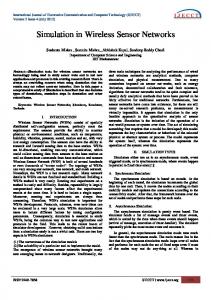
Fig. 1. The phase update of “own” node (node under consideration) during its th firing cycle when: (a) the next fire message is received in DESYNC, with the node’s listening interval defined as the time between the fire message preceding and following its own firing; (b) a fire message is received in PCO-based ). desynchronization while the node’s own phase is within its listening interval (i.e., when
II. DESYNCHRONIZATION PRIMITIVES A. Notations and Symbolism Italicized letters indicate scalars and boldface letters indicate vectors. For vectors and , the circular convolution [34] with period is given by
Random variables (RVs) are represented by Greek uppercase letters, e.g., or , with and reserved to indicate the normal and uniform probability density functions (PDFs), respectively, with mean (and ) and standard deviation (and ). The mathematical operators and key concepts used in the paper are summarized in Table I. B. Introduction to Desynchronization Consider a WSN comprising fully-meshed nodes, i.e., every WSN node can receive message broadcasts from all other nodes. Each node in the WSN is an “oscillator” that performs a task with a period of seconds [4]. In the beginning, each node sets its internal timer to a random initial value between . Upon the completion of its cycle, each node broadcasts a fire message and immediately resets its internal timer to zero. In the steady (desynchronized) state, each node fires every seconds. For each node, its firing cycle comprises the time duration in-between two sequential fire message transmissions of its own. For each node, the percentage of the way through its th firing cycle is denoted as the node’s own firing phase [2]–[4], [14], [20], [31], [32], . In order to achieve convergence to steady state, beyond its own phase, each node counts the percentage of time from the moments it receives fire messages from other nodes and updates its own phase according to the desynchronization primitives detailed in the next two subsections. Each node listens for fire message broadcasts within a certain interval before (and possibly after) its own firing, which is termed as the listening interval. Following the schema of Degesys et al. [4], the fire messages’ phase values can be imagined as beads moving clockwise on a
ring with period s (Fig. 1). When a node’s own firing phase reaches unity, i.e., top of Fig. 1, the node broadcasts a fire message and the node’s own firing phase is reset to zero. The figure illustrates a node’s own firing phase during its th firing cycle and Fig. 1(a) shows the phase of the received fire messages from the two nodes that fired immediately before and after it, denoted by and , respectively1. Thus, superscripts always indicate the firing cycle of “own” node in the WSN (i.e., of the node under consideration) and subscripts indicate the order relative to “own” node. The nodes corresponding to the previous and next firings of “own” node are called phase neighbors and the listening interval corresponding to the th firing of “own” node is illustrated in Fig. 1. For all desynchronization algorithms under consideration [3], [4], [9], [12], [20], [23], [26], [32]: 1) the notion of phase neighbors indicates temporal adjacency of fire messages and is independent of the nodes’ physical location; 2) it is immaterial which physical sensor node is linked to which fire message, as desynchronization is solely dependent on the received fire message phase. Therefore, the analysis of this paper is presented from the viewpoint of any single node in the WSN [20], [22], [25] and does not need to discern the specific firing order of all nodes in the network, which in fact may not be constant during the desynchronization convergence process. C. DESYNC In this approach, each node updates its firing phase once within each of its firing cycles, at the moment when the next fire message is received. As shown in Fig. 1(a), each node listens for the fire message preceding and following its own fire message broadcast. Hence, the duration of each node’s listening interval depends on the relative times inbetween these two messages. It then performs its phase update during its th firing cycle based on the phases of these two received and . Specifically, each node’s phase messages, i.e., update moves its own firing phase towards the middle of the 1In this section, we ignore the phase measurement noise and assume each fire time can be determined precisely by all receiving nodes. This noise is however taken into account in the modeling framework.
224
IEEE TRANSACTIONS ON SIGNAL PROCESSING, VOL. 63, NO. 1, JANUARY 1, 2015
listening interval2. The phase update of DESYNC during the th firing cycle is expressed by [4], [9]
a node [3] is performed at last fire message broadcast,
seconds after the node’s : (4)
(1) where denotes the phase-coupling constant that controls the speed of the phase adaptation. Previous work [4], [9] showed that the reactive listening primitive of (1) disperses all fire message broadcasts at intervals of . Thus, after firing cycles, the DESYNC algorithm leads to fair TDMA scheduling, where all fire messages in the network are periodic and the phase update of (1) leads to convergence to SState, expressed by
(2) the preset convergence threshold, typically [3], [4], with [14], [20], [31], [32] . In a practical WSN deployment [4], [24], [25], [32], [33], each node would check that the condition of (2) holds for several consecutive firing cycles beyond (e.g., five cycles) and would then declare that convergence has been achieved. In steady state, each node transmits data packets for seconds immediately following its fire message broadcast (which limits the maximum number of nodes supported under TDMA to less than ). The only overhead stems from the fire message broadcasts, which are very short packets (just two bytes in our implementation). Assuming negligible propagation delay and error-free detection of messages, it has been conjectured via simulations [3], [4] that convergence requires iterations of the order (3) Even though the order estimate (3) gives a coarse characterization for the convergence iterations, it cannot provide the expected number of iterations until convergence to SState is achieved. Moreover, real-world experimentation with TelosB and iMote2 motes [4], [32] under fixed and values show that the measured number of iterations until convergence to SState is not proportional to . D. PCO-Based Inhibitory Coupling PCO-based desynchronization with inhibitory coupling updates each node’s own firing phase according to the received fire messages within a certain interval of its firing cycle [3]. This is termed as the listening interval and its positioning within the th firing cycle of a node is illustrated Fig. 1(b). As such: (i) the phase of the node’s own firing changes after a fire message from a previous phase-neighbor is received within the listening interval (i.e., unlike DESYNC, a varying number of phase updates may occur within each firing cycle); (ii) knowledge of the total number of nodes is required [3]. Hence, a phase update during the th firing cycle of PCO-based desynchronization of
where the phase-coupling constant controlling the speed of the phase adaptation. All fire messages received outside the listening interval are simply ignored. After firing cycles, (4) has been shown to converge to dispersed fire message broadcasts received at intervals of seconds [3], i.e., (2) holds under convergence to SState. Hence, like in the DESYNC case, once fair TDMA is achieved, the only overhead stems from the short fire message broadcasts. Assuming negligible propagation delay, error-free detection of broadcast messages and that , it has been shown [3] that the number of firing cycles for convergence is lower bounded by (5) Nevertheless, the tightness of (5) has neither been proven nor demonstrated via real-world experiments or simulation results. III. PROPOSED STOCHASTIC MODELING OF DESYNC AND PCO-BASED DESYNCHRONIZATION WITH INHIBITORY COUPLING Assumption 1 (Fully-Meshed Topology): We consider fullymeshed networks where each node can directly receive the fire message broadcasts from all other nodes. When performing the first phase update of (1) and (4), each node’s own firing phase, as well as the phases of all received fire messages from its phase neighbors, are modeled by independent . This is random variables that are uniformly distributed in formally stated in the following assumption. Assumption 2 (Phase Model): For every node under consideration (“own” node) and its phase neighbors, their firing phase during the first phase update is modeled by: , with3 (6) We define the mean times of successive phase updates to be equidistant, which, for the DESYNC update of (1), is expressed as (7) and for the PCO update of (4) is stated by (8) In the beginning of the desynchronization process, all fire message broadcasts are completely uncoordinated (random), i.e., .
2Since (1) is applied
at the moment when the next firing is received, we have: , as seen in Fig. 1(a); however, we include in (1) to clarify that the operation of DESYNC depends on both the previous and next firing phase.
3The use of the modulo operator in (6) is imposed because, by definition, we . must ensure
BURANAPANICHKIT et al.: CONVERGENCE OF DESYNCHRONIZATION PRIMITIVES IN WIRELESS SENSOR NETWORKS
We remark that there is no loss of generality from the assumption of equidistant means of (7) and (8) as the modulo operator of (6) ensures that the PDFs wrap around one such that for every node and are always uniformly-distributed between irrespective of the assumed mean values. However, we opt for the use of (7) and (8) as this facilitates the mathematical exposition of the proposed estimates. Our estimates of the convergence iterations for DESYNC and PCO-based desynchronization assume that each phase in (1) and (4) is contaminated by white noise due to the varying propagation, mobility and node processing delays of a WSN environment. This is captured in the following assumption. Assumption 3 (Measurement Noise Model): All phase values in the update of (1) or (4) are contaminated by additive noise, modeled by an independent, zero-mean, uniformly-distributed, random variable, . The assumption of uniform distribution for the measurement noise, as well as the value of the standard deviation will be derived experimentally, as they incorporate the effects of interference, wireless propagation and processing delays that can only be inferred via measurements from a real setup. Due to the measurement noise and the interaction between fire message broadcasts, for each phase update of each node’s firing phase, , during its th firing cycle, the PDF of , changes after applying (1) or (4). Consequently, this changes the probability of convergence to SState, as follows:
225
right-hand side of (11). That is, we determine the firing cycle leading to convergence to SState with probability that closely matches , which is our (predetermined) confidence. Definition 1 (Steady State): We define a desynchronization primitive as being in steady state with % confidence, at the th firing cycle, , where (13) the standard deviation of a node’s own firing phase with PDF at the application of the updates of (1) or (4) during its th firing cycle. Since is affected by measurement noise, in order for the system to remain in the converged state indefinitely, the , must be set according to threshold for the convergence, the (estimated) . Conversely, we can treat the entire desynchronization process as a “black box” system and estimate by measuring the phase deviation from the mean obtained when performing the update of (1) or (4) during SState. This will be demonstrated in the experimental section. A. Modeling of DESYNC Convergence Proposition 1: Under Assumptions 1–3, the expected number of firing cycles for the DESYNC phase update of (1) to converge according to Definition 1 is
(14) with (9) where is the error function [35]. Noconverges tice that (9) holds under the assumption that to a normal distribution for both DESYNC and PCO-based desynchronization, which, as the next two subsections will show, turns out to be the case. We therefore use a stochastic criterion for convergence based on the confidence intervals of the normal distribution [35]. By defining the confidence coefficient
(10) and replacing in (9), we get (11)
(15)
and (16) being the vector produced by consecutive circular convolutions of period . Proof: Consider any single node in the WSN. We denote the initial phase random variables corresponding to the node under consideration by the vector (17)
with the inverse error function that can be computed by its Maclaurin series
The corresponding additive measurement noise sources [independent identically distributed (i.i.d.) random variables from Assumption 3] are denoted by the vector
(12)
(18)
Thus, (11) becomes the mechanism for defining the phase update iteration leading to SState. Specifically, we determine the firing cycle for which is closest to the
and Evidently, the number of elements before and after in (17) and (18) depends on how many fire message broadcasts (firings) precede or follow the node’s own firing
226
IEEE TRANSACTIONS ON SIGNAL PROCESSING, VOL. 63, NO. 1, JANUARY 1, 2015
during its initial firing cycle. The first phase update of (1) is expressed stochastically as
B. Modeling of PCO-Based Convergence Proposition 2: Under Assumptions 1–3, the expected number of firing cycles for the PCO-based phase update of (4) to converge according to Definition 1 is
(19) and corNotice that (19) imposes that the statistics of respond to the initial firing cycle (Assumption 2). This is because, during each phase update, we do not take into account nodes’ phase updates that may have been carried out during the first firing cycle. This corresponds to the operational form of the DESYNC algorithm (i.e., “DESYNC stale” of [4], [20]). It is straightforward to derive from (19) that remains unchanged after the first phase update, while the standard deviation is modified to:
(24) with (25) and
,
(20) (26)
Furthermore, by writing (19) for all the phase elements of given in (17), we reach (21) The circular convolution performs periodic extension of the phase and noise vectors of (17) and (18), which corresponds to the circular dependency between consecutive firing cycles 4. Generalizing (21) to the th firing cycle, we reach
Proof: We separate the proof into three parts, based on the temporal evolution of the convergence process. We present here the main part of the proof, which comprises the analysis of the first firing cycle and the derivation of the th phase update of a node during its th firing cycle in PCO, while the remaining details to complete the proof are given in Appendix B. First firing cycle: Consider any single node in the WSN. The expected number of phase updates it will perform within its first firing cycle is equal to the number of fire message broadcasts (firings) expected to be heard by the node within , which is
(22) (27) is the i.i.d. measurement noise vector per iteration. where Therefore, we obtain: and shown in becomes normally dis(15). It can now be shown that tributed after a few firing cycles (see Appendix A), i.e.,
This stems from the binomial theorem, since Assumption 2 mandates that the initial phase of each node is uniformly distributed within . Via (4), a phase update during the first firing cycle of a node can be expressed stochastically as
(23) Hence, we reach (14) for convergence under Definition 1. Proposition 1 shows how is affected by as well as by the initial conditions and the noise assumptions expressed by and in Assumptions 2 and 3, respectively. Interestingly, according to (14), the number of nodes, , does not appear to influence the convergence to the steady state. This is in contrast to the conjecture of Degesys et al. [3], [4] given by (3). Nevertheless, experimental results given in the next section will demonstrate that real-world WSNs, as well as simulation results, are in agreement with Proposition 1. 4For the special cases of nodes, we set convolution of (16) to avoid erroneous overlapping within period of the circular convolution.
in the circular due to the short
(28) the random variable modeling the measurement with noise (Assumption 3) of the node’s own phase. From (8) and (28) we obtain (29) i.e., the mean values of successive fire message updates remain equidistant after the first firing cycle of a node. The standard deviation of after the update of (28) is (30)
BURANAPANICHKIT et al.: CONVERGENCE OF DESYNCHRONIZATION PRIMITIVES IN WIRELESS SENSOR NETWORKS
Generalizing (28) to the th phase update of the th firing cycle of a node, leads to
(31) i.i.d. random variables, each stemming from Aswith is given by (29) and its standard sumption 3. The mean of deviation is given by (26). Similarly to Proposition 1, it can be shown that becomes a normally-distributed random variable after a few phase updates (see Appendix A). We can thus reach convergence under Definition 1 for given by (25). However, given that in PCO-based desynchronization the number of phase updates per firing cycle is not fixed, i.e., in general, , in order to derive the expected number of firing cycles until a node converges to steady state, we need to derive the expected number of phase updates after each firing cycle. We can then match the number of phase updates expected to take place until convergence to the corresponding number of firing cycles. The details of this process and the proof of (24) are given in Appendix B. Proposition 2 shows that is affected by , as well as by the initial conditions and the noise assumptions, expressed by and in Assumptions 2 and 3. The total number of nodes, , is also influencing the number of iterations for convergence to the steady state. However, as it will be shown by the next section (experiments), this effect is negligible in practice. This is in contrast to the lower bound derived by Pagliari et al. [3], given by (5). However, the experimental results of the next section will demonstrate that real-world WSNs, as well as simulation results, are in agreement with Proposition 2. IV. EXPERIMENTAL VALIDATION For our experiments, we used iMote2 Crossbow sensors with TinyOS1.x. All nodes use the IEEE 802.15.4 standard with the default 2.4 GHz Chipcon CC2420 wireless transceiver. We followed the TinyOS standard message format but reduced it to two data bytes when sending fire messages. Similar to prior work [4], we set the backoff time to 1.2 ms. A. Standard Deviation of the Phase Measurement Noise The test environment was a standard university laboratory room. Our approach for measuring was carried out as follows: (i) we implemented the DESYNC and PCO-based desynchronization in TinyOS nesC code as described in Section II; (ii) we set to ensure maximum coupling strength and s (this period value was used in all our experiments) and (iii) we measured the oscillatory behavior of each node’s phase after the WSN was left operating for a prolonged interval of time (during which nodes were occasionally moved within the test area) to ensure convergence to SState. The statistics of the oscillatory phase behavior, observed via this experiment, express the cummulative effects of interference, mobility and clock drift amongst nodes. This approach is easy to replicate under any
227
real-world WSN setup involving varying levels of interference or node mobility [7], [12], [26]. For both algorithms, we found the standard deviation of the oscillating phase amplitude around the SState value of each node’s phase to be ms and the accumulated phase statistics over all nodes were confirmed as marginally white. This validates our noise assumption stated in Assumption 3. The derived value for was used during the experimental validation of Proposition 1 and Proposition 2. No other parameter tuning is needed for the proposed model. B. Measurement and Simulation Setup In both DESYNC and PCO-based desynchronization, once all nodes were activated to transmit and receive on a single channel, a special “mix message” was broadcast by one of the nodes (chosen randomly) in order to trigger all nodes to set their initial fire message phase to a random interval within s from its reception. This creates the initial conditions of Assumption 2. The nodes will then desynchronize their transmission of fire messages and converge to fair TDMA scheduling. We present results under two convergence thresholds, i.e., and , with coupling constants and number of nodes . We use to detect convergence under Definition 1 with near certainty. Finally, we have experimented with various settings for the firing period and all such experiments led to very similar results for the convergence iterations to the SState. Thus, all reported experiments use firing period of s, which complies with previous work [3], [4], [10], [12], [20]. Under this setup, each node detects convergence to SState by checking if (2) is valid for its last ten firing cycles. After achieving SState and remaining in this state for 50 firing cycles, a node broadcasts another mix message, in order to repeat the process. Each node reported the number of its firing cycles until convergence was detected (minus nine cycles) via a special “report” message to a base station listening passively to all messages for monitoring purposes. This facilitated the automated collection of 50 such results per number of nodes, threshold and coupling constant. In order to cross-validate our theoretical and experimental results with simulations, we used the Matlab code of Degesys et al. [4] for DESYNC and added to it Matlab code for PCO with inhibitory coupling. In order to simulate the noise conditions observed in our experimental setup, we deliberately apply zero-mean additive noise in each phase update with ms and set each node to misfire with probability 0.4%. Despite the fact that the simulation cannot capture the complex behavior of the real system in full detail, it allows for numerous desynchronization processes to be simulated (300 Matlab runs per triplet for each algorithm). C. DESYNC Results he results for this desynchronization mechanism are reported in Fig. 2. All measurements around a value of correspond to results with that value of ; they have been plotted slightly separately solely for ease of illustration. For comparison purposes, we have also included the order-of-convergence conjecture of
228
IEEE TRANSACTIONS ON SIGNAL PROCESSING, VOL. 63, NO. 1, JANUARY 1, 2015
Fig. 2. Required firing cycles for convergence to SState for the DESYNC algorithm for various values of . The vertical error bars correspond to one standard , (b) DESYNC, deviation from the experimental (or simulation) mean values, which are indicated by marks. (a) DESYNC, , (c) DESYNC, , (d) DESYNC, , (e) DESYNC, , (f) DESYNC, .
(3) [3], [4] in our results, by scaling the order estimate to fit within the range of the obtained experiments and simulations. The results of Fig. 2 show that the WSN tends to converge to steady state faster when decreases (until ), since the presence of measurement noise causes higher-amplitude perturbations for strong coupling, i.e., for high values of . However, for very small values of , the convergence iterations increase dramatically due to weakened coupling between phase-neighboring nodes. Moreover, by comparing the convergence results for low and high convergence threshold , one can observe that the use of small convergence threshold increases the required convergence iterations to SState. The proposed model predicts these trends in the convergence iterations accurately. Specifically, the estimate of Proposition 1 is within one standard deviation of the experimental and simulation results for the vast majority of cases. The Pearson correlation coefficients for the proposed model curves against the
mean experimental values (averaged over ) were found to be 0.9893 and 0.9931 for and , respectively. The corresponding Pearson correlation coefficients for the conjecture of (3) from [4], [3] were 0.8639 and 0.9464. These results underline the superior estimation accuracy of our approach. Finally, the experimental results of Fig. 2 show no statistical dependence on , which agrees with Proposition 1. D. Results With PCO-Based Desynchronization The results are reported in Fig. 3 for both small and large convergence thresholds. Since (5) provided negative estimates for most values of , we added an offset to the results of the bound to bring as many as possible to the non-negative region and present only the non-negative ones. Evidently, the bound of (5) does not match the observed behavior. We remark however that this is to be expected, as the bound of (5) is derived under
BURANAPANICHKIT et al.: CONVERGENCE OF DESYNCHRONIZATION PRIMITIVES IN WIRELESS SENSOR NETWORKS
229
Fig. 3. Required firing cycles for convergence to SState for the PCO-based algorithm for various values of . The vertical error bars correspond to one standard , (b) PCO, , deviation from the experimental (or simulation) mean values, which are indicated by marks. (a) PCO, , (d) PCO, , (e) PCO, , (f) PCO, . (c) PCO,
the assumption that each firing is influenced only by the firing of one phase-neighboring node [3]. Fig. 3 shows that, in PCO, the convergence iterations decrease monotonically with . The proposed model predicts this trend correctly and, remains within one standard deviation from the majority of the experimental and simulation results. The model results do not change5 for different values of , which agrees with the overall experimentally-observed behavior of the system. Finally, by comparing the convergence results for low and high convergence threshold, we note that the use of small convergence threshold increases the required convergence iterations to SState. The proposed model predicts this behavior correctly and agrees with the experimental trends reported. The Pearson correlation coefficients for the model curves against the 5i.e., Proposition 2 leads to the same results for the convergence iterations under different values of
mean experimental values were 0.9739 for 0.9989 for .
and
E. Discussion By cross referencing between Figs. 2 and 3 we can compare the convergence iterations of both algorithms under different settings. Under appropriate choice for the coupling coefficient, , the required firing cycles for convergence with PCO-based desynchronization is comparable to those of DESYNC. In addition, we can make the following observations. • Accuracy of previous analytic work on estimation of convergence iterations: Previous estimates or bounds must be scaled to fit the range of the experimental values, as they are either order-of-convergence estimates [i.e., (3)], or overly optimistic bounds [i.e., (5)]. Moreover, as illustrated in Figs. 2 and 3, when varying the coupling parameter ,
230
•
•
•
•
IEEE TRANSACTIONS ON SIGNAL PROCESSING, VOL. 63, NO. 1, JANUARY 1, 2015
previous estimates do not accurately match the behavior observed in the experimentally-obtained convergence iterations. Impact of measurement noise: Contrary to the proposed model, these previous estimates do not take into account the measurement noise conditions. Independently from this work, and following different analysis and modeling approaches, recent work in synchronization [29], [30] and desynchronization [10] has shown that noise in the desynchronization phase update (e.g., by quantization) and drops (or collisions) of beacon messages can affect the convergence iterations and can lead to convergence iterations that deviate from the estimates obtained based on the ideal (noise-free) model assumed by earlier work. Generalization to non-uniformly distributed initial firings: In Propositions 1 and 2, every node’s initial phase random variable was assumed to be i.i.d. uniform via Assumption 2. However, Propositions 1 and 2 hold for any i.i.d. random variable that satisfies the three conditions for the generalized form of the central limit theorem to be applicable [35, pp. 219–220] (see Appendix A). Utilized desynchronization algorithm and the network topology: While we focused on the initial desynchronization proposals with limited listening, recent work has extended these initial paradigms towards other frameworks, where nodes adjust their own firing phase based on larger listening intervals and/or via the usage of anchored (i.e., non-adjusting) nodes [10]–[12], [21], [23], [25], [26]. While we do not investigate the applicability of our modeling approach to all such frameworks, our analysis includes the coupling parameter and adjusts according to the node firings received within the predetermined listening interval. It is also worth noting that Propositions 1 and 2 cover the important scenario of a fully-meshed (all-to-all) WSN. Desynchronization extensions to multihop scenarios have been investigated by several works [20]–[22]. Given that there is a large variation in the topologies to consider and that it has been shown that the steady-state difference between the phases of consecutive firings, as well as the average number of convergence iterations, varies depending on the network topology under consideration [21], [22], [25], [30] (due to the “selective” listening of beacons stemming solely from non-hidden nodes), we do not investigate the validity of our analysis to such cases. However, we remark that this could be attempted following the same approach as for Propositions 1 and 2, if the topology specification is known a-priori. Consideration of phase updates performed during each node’s firing cycle: As mentioned in the proof of Proposition 1, to calculate and its moments for DESYNC and PCO-based convergence, our analysis does not take into account the variability in the neighboring nodes’ phase updates6. This is in agreement with the way DESYNC is applied in practice and constitutes a simplification for PCO-based desynchronization [3], [4]. Given that our
6e.g., updates that may have been carried out during the th firing cycle of the node under consideration, or variability due to misfiring or other non-idealities not captured by our noise assumption (Assumption 2)
stochastic modeling framework is in good agreement with the average experimental and simulation results without requiring experimental tuning (besides knowledge of the standard deviation of the phase measurement noise), our approach forms an important step towards considering stochastic models for the convergence of desynchronization systems. V. APPLICATION EXAMPLES The proposed stochastic estimation framework can benefit desynchronization-based TDMA protocols in WSNs by analytically estimating the impact of the phase-coupling constant , convergence threshold and firing cycle period on such deployments [3], [4], [32]. We present two such examples. A. Maximizing the Bandwidth Per Node In the first case, we consider a WSN that initially comprises nodes, where nodes are expected to join or leave the network every seconds. This scenario usually occurs when mobile nodes periodically enter and exit the coverage area of the network, or some nodes switch on and off periodically to conserve energy. In fair TDMA scheduling, the bandwidth per node is bps, where is the maximum applicationlayer bandwidth7 in IEEE 802.15.4. In practice, the fluctuating number of nodes in the WSN will result in bandwidth loss as, each time nodes join or leave, the system needs to converge to SState before transmission resumes with equal slot size [4], [32], [33]. Using the proposed framework, we can derive an estimate of the expected bandwidth per node under such conditions. Specifically, if the PCO or DESYNC firing-cycle period is seconds and the node joining or exiting occurs (on average) every seconds, the expected bandwidth per node can be estimated as
(32) with the expected firing cycles until convergence to SState, given by Proposition 1 or Proposition 2. The factor in (32) expresses the normalized loss of bandwidth per node due to convergence to TDMA under DESYNC and PCO every time nodes join or leave the network. Using the experimental setup of Section IV, we present an example of the calculation of (32) for a WSN comprising nodes with s and 1–3 nodes entering or exiting the network every seconds, with to incorporate up to 30% variability around the mean value of 100 s. The maximum application-layer bandwidth was measured to be kbps. Tables II and III present the results when using the value of that was estimated to provide the minimum under Propositions 1 and 2 against the result when using values for suggested from previous work. It is evident that, for all cases, the proposed model provides the setting for that minimizes the convergence iterations and leads to the maximum achievable bandwidth per node. This is despite the fact 7Following the approach of Degesys [4], we estimate by using a single transmitter and receiver to measure the achieved delivery rate at the application layer.
231
BURANAPANICHKIT et al.: CONVERGENCE OF DESYNCHRONIZATION PRIMITIVES IN WIRELESS SENSOR NETWORKS
TABLE II DESYNC: AVERAGE BANDWIDTH PER NODE,
PCO: AVERAGE BANDWIDTH PER NODE,
(IN
KBPS), UNDER DIFFERENT CONVERGENCE PHASE-COUPLING CONSTANT
THRESHOLDS
AND
DIFFERENT VALUES
FOR THE
TABLE III (IN KBPS), UNDER DIFFERENT CONVERGENCE THRESHOLDS AND DIFFERENT VALUES FOR THE PHASE-COUPLING CONSTANT
TABLE IV DESYNC AND PCO FOR DESIRED CONVERGENCE TIME OF 10 S. THE CORRESPONDING FIRING CYCLE PERIOD, THE “THEORETICAL” COLUMNS
that the model assumes uniformly-distributed initial fire times, while in the application results the values of most nodes may be (approximately) equidistant at the moment 1–3 nodes enter or exit the network. The impact on the achieved bandwidth per node is much more pronounced in the case of DESYNC, where previous work used instead of the best option, which is . The results in Tables II and III, show that selecting through the proposed model brings gains of up to 13% in the bandwidth per node compared with the standard settings used in existing works [4], [3]. B. Estimating the Required Firing Cycle Period In the second application example, we focus on the case of a WSN using DESYNC or PCO and requiring convergence to steady state to be achieved within seconds on average. The desired value of depends on the application context, e.g., a predefined value in order to limit the delay and buffering requirements between the data acquisition and transmission when the WSN is activated [13], [32], [33]. Based on Proposition 1 and Proposition 2, and under given settings for and , we can match the period of firing cycles to the desired convergence time by: . By solving the last equation for we derive the firing cycle period that meets the convergence time expectation under given by Proposition 1 and Proposition 2 for each setting of and . We have experimented with various parameters of DESYNC or PCO and the obtained theoretical and experimental results are reported in Table IV using the average obtained from multiple runs with . With the exception of two cases (DESYNC at: and PCO at:
, IS GIVEN IN PARENTHESES (IN SECONDS) IN
), the theoretical prediction is within a 25% margin of the experimentally observed convergence time. VI. CONCLUSION A novel stochastic estimation framework for the convergence iterations to fair TDMA scheduling is proposed for the two desynchronization primitives with limited listening, namely, DESYNC and pulse-coupled oscillators with inhibitory coupling. Our stochastic estimates establish the expected firing cycles until each node’s firing converges to the steady state with very high confidence. For both algorithms, our analytic expressions are validated based on simulations and experiments with a fully-meshed network of wireless sensors. The results show that our estimates are more accurate than previous order-of-convergence estimates and lower bounds. Our model incorporates the influence of system parameters (i.e., total number of nodes, coupling coefficient, convergence threshold and phase measurement noise) on the expected convergence iterations. Therefore, it can be used to estimate the best operational parameters (and the associated delay) to establish fair TDMA scheduling under several desynchronization-based WSN protocols. More broadly, the analysis of this paper contributes towards the analytic understanding of how a desynchronization system is expected to evolve from random initial conditions to the desynchronized steady state. APPENDIX A We show that of (22) and (31), i.e., the RV modeling each node’s own phase during its th firing cycle under DESYNC and PCO (respectively), is normally distributed after a few phase updates.
232
IEEE TRANSACTIONS ON SIGNAL PROCESSING, VOL. 63, NO. 1, JANUARY 1, 2015
Moreover, the probability that listening interval is
Fig. 4. A pictorial illustration of the PDFs of the phase RVs of the th firing cycle of “own” node, during “own” node’s th phase update, performed via (4).
Once (22) and (31) are reached, we can make the following observations: • is a linear mixture of independent random variables, i.e.: (i) i.i.d. noise and phase vectors and in and in PCO; DESYNC; (ii) • for DESYNC: , we can pick and, from (15), ; ; • for PCO: • all initial PDFs have finite support (they are all variants of the uniform distribution); hence, densities will have finite support since they are linear mixtures of PDFs with finite support. These observations satisfy the three conditions for the generalized form of the central limit theorem to be applicable becomes a normally-dis[35, pp. 219–220], and thus tributed random variable after a few phase updates. Papoulis [35, pp. 219–220] suggests that the normal PDF is accurately approximated with just five linear combinations of PDFs satisfying the above criteria, meaning that five phase updates will suffice for the normal distribution to be an accurate approximation of the firing phase of each node.
APPENDIX B We present the analysis that matches the expected number of phase updates until convergence to the expected number of firing cycles and concludes the proof of (24). Subsequent firing cycles, effect of phase-neighboring firings: A pictorial illustration of the PDF of the th phase update of a node (performed during its th firing cycle, with ) is given in Fig. 4 in conjunction with its listening interval and the PDFs of the two previous firings and the next firing. Since all phase RVs are normally distributed after a few phase updates, it is straightforward to infer from Fig. 4 that the probability for the previous firing (represented by RV ) to occur within the listening interval is
will occur within the node’s
This is also the probability that will occur within the node’s listening interval. Subsequent firing cycles and the effect of all firings within a window of firing events: We can now generalize the previous calculation to the probability of occurrence of the previous and next firings within the node’s listening interval. Beyond the previous firing, for the th firing after the node’s own firing or the th firing before the node’s own firing , this probability is
Hence, summing up the probabilities of firings occurring within the node’s listening interval for all firings before and after the current one, the expected number of phase updates is given by the expression in the summation term of (24), where we used the identity :
(33) The expected number of phase updates within of a node is
firing cycles
As a result, for phase updates leading to convergence under Definition 1 [shown by (25)], the corresponding number of firing cycles is given by (24). REFERENCES [1] O. Simeone, U. Spagnolini, Y. Bar-Ness, and S. Strogatz, “Distributed synchronization in wireless networks,” IEEE Signal Process. Mag., vol. 25, no. 5, pp. 81–97, Sep. 2008. [2] R. Leidenfrost and W. Elmenreich, “Firefly clock synchronization in an 802.15.4 wireless network,” EURASIP J. Embed. Syst., vol. 2009, p. 17, 2009, Article id. 18585. [3] R. Pagliari, Y.-W. Hong, and A. Scaglione, “Bio-inspired algorithms for decentralized round-robin and proportional fair scheduling,” IEEE J. Sel. Areas Commun., vol. 28, no. 4, pp. 564–575, May 2010. [4] J. Degesys, I. Rose, A. Patel, and R. Nagpal, “Desync: Self-organizing desynchronization and tdma on wireless sensor networks,” in Proc. 6th Int. Symp. IPSN, Apr. 2007, pp. 11–20. [5] A. Mutazono, M. Sugano, and M. Murata, “Energy efficient self-organizing control for wireless sensor networks inspired by calling behavior of frogs,” Comput. Commun,, vol. 35, no. 6, pp. 661–669, 2012.
BURANAPANICHKIT et al.: CONVERGENCE OF DESYNCHRONIZATION PRIMITIVES IN WIRELESS SENSOR NETWORKS
[6] H. Yamamoto, N. Wakamiya, and M. Murata, “An inter-networking mechanism using stepwise synchronization for wireless sensor networks,” in Bio-Inspired Models of Network, Information, and Computing Systems. Berlin, Germany: Springer-Verlag, 2012, pp. 276–287. [7] T. Nakano, “Biologically inspired network systems: A review and future prospects,” IEEE Trans. Syst., Man, Cybern., C, Appl. Rev., vol. 41, no. 5, pp. 630–643, Sep. 2011. [8] J. Klinglmayr and C. Bettstetter, “Self-organizing synchronization with inhibitory-couples oscillaotrs: Convergence and robustness,” ACM Trans. Autonom. Adapt. Syst., vol. 7, no. 3, Sep. 2012. [9] A. Patel, J. Degesys, and R. Nagpal, “Desynchronization: The theory of self-organizing algorithms for round-robin scheduling,” in Proc. IEEE Int. Conf. Self-Adaptive Self-Organizing Syst. (SASO’07), Jul. 2007, pp. 87–96. [10] S. Ashkiani and A. Scaglione, “Discrete Dithered Desynchronization,” 2012 [Online]. Available: arXiv preprint arXiv:1210.2122 [11] S. Choochaisri, K. Apicharttrisorn, K. Korprasertthaworn, P. Taechalertpaisarn, and C. Intanagonwiwat, “Desynchronization with an artificial force field for wireless networks,” ACM SIGCOMM Comput. Commun. Rev., vol. 42, no. 2, pp. 7–15, 2012. [12] C. Lien, S. Chang, C. Chang, and D. Lee, “Anchored desynchronization,” in Proc. IEEE INFOCOM’12, 2012, pp. 2966–2970. [13] I. Bojic, V. Podobnik, I. Ljubi, G. Jezic, and M. Kusek, “A self-optimizing mobile network: Auto-tuning the network with fireflysynchronized agents,” Inf. Sci., vol. 182, no. 1, pp. 77–92, 2012. [14] R. Pagliari and A. Scaglione, “Scalable network synchronization with pulse-coupled oscillators,” IEEE Trans. Mobile Comput., vol. 10, no. 3, pp. 392–405, Mar. 2011. [15] R. E. Mirollo and S. H. Strogatz, “Synchronization of pulse-coupled biological oscillators,” SIAM J. Appl. Math., vol. 50, no. 6, pp. 1645–1662, 1990. [16] P. C. Bressloff and S. Coombes, “Desynchronization, mode locking, and bursting in strongly coupled integrate-and-fire oscillators,” Phys. Rev. Lett., vol. 81, no. 10, p. 2168, 1998. [17] S. R. Campbell, D. L. Wang, and C. Jayaprakash, “Synchrony and desynchrony in integrate-and-fire oscillators,” Neural Comput., vol. 11, no. 7, pp. 1595–1619, 1999. [18] Y. Kuramoto, Chemical Oscillations, Waves, and Turbulence. Mineola, NY, USA: Dover Publications, 2003. [19] A. Arenas, A. Diaz-Guilera, J. Kurths, Y. Moreno, and C. Zhou, “Synchronization in complex networks,” Phys. Rep., vol. 469, no. 3, pp. 93–153, 2008. [20] J. Degesys and R. Nagpal, “Towards desynchronization of multi-hop topologies,” in Proc. IEEE Int. Conf. Self-Adapt. Self-Organizing Syst. (SASO’08), 2008, pp. 129–138. [21] A. Motskin, T. Roughgarden, P. Skraba, and L. Guibas, “Lightweight coloring and desynchronization for networks,” in Proc. IEEE INFOCOM’09, 2009, pp. 2383–2391. [22] H. Kang and J. L. Wong, “A localized multi-hop desynchronization algorithm for wireless sensor networks,” in Proc. IEEE INFOCOM’09, 2009, pp. 2906–2910. [23] D. De Guglielmo, G. Anastasi, and M. Conti, “A localized desynchronization algorithm for periodic data reporting in ieee 802.15. 4 wsns,” in IEEE Symp. Comput. Commun. (ISCC’12), 2012, pp. 605–610. [24] Y. Wang, F. Nunez, and F. Doyle, “Statistical analysis of the pulsecoupled synchronization strategy for wireless sensor networks,” IEEE Trans. Signal Process., vol. 61, no. 21, pp. 5193–5204, 2013. [25] C. Muhlberger, “Analyzing a self-organizing multi-hop protocol: Ease of simulations and need for real-world tests,” in Proc. 9th IEEE Int. Conf. Wireless Comm. Mob. Comp., IWCMC, 2013. IEEE, 2013, pp. 1029–1034. [26] T. Settawatcharawanit, S. Choochaisri, C. Intanagonwiwat, and K. Rojviboonchai, “V-desync: Desynchronization for beacon broadcasting on vehicular networks,” in Proc. IEEE Veh. Technol. Conf. (VTC Spring), 2012, pp. 1–5. [27] A. Cornejo and F. Kuhn, “Deploying wireless networks with beeps,” Distrib. Comput., vol. 182, no. 1, pp. 148–162, 2010. [28] Y. Wang, F. Nunez, and F. Doyle, “Energy-efficient pulse-coupled synchronization strategy design for wireless sensor networks through reduced idle listening,” IEEE Trans. Signal Process., vol. 60, no. 10, pp. 5293–5306, Oct. 2012. [29] J. Klinglmayr, C. Kirst, C. Bettstetter, and M. Timme, “Guaranteeing global synchronization in networks with stochastic interactions,” New J. Phys., vol. 14, no. 7, p. 073031, 2012.
233
[30] J. Nishimura and E. J. Friedman, “Probabilistic convergence guarantees for type-ii pulse-coupled oscillators,” Phys. Rev. E, vol. 86, no. 2, p. 025201, 2012. [31] Y.-W. Hong, A. Scaglione, and R. Pagliari, “Pulse coupled oscillators’ primitive for low complexity scheduling,” in Proc. IEEE Int. Conf. Acoust., Speech, Signal Process. (ICASSP’09), 2009, pp. 2753–2756. [32] D. Buranapanichkit and Y. Andreopoulos, “Distributed timefrequency division multiple access protocol for wireless sensor networks,” IEEE Wireless Commun. Lett., vol. 1, no. 5, pp. 440–443, Oct. 2012. [33] H. Besbes, G. Smart, D. Buranapanichkit, C. Kloukinas, and Y. Andreopoulos, “Analytic conditions for energy neutrality in uniformlyformed wireless sensor networks,” IEEE Trans. Wireless Commun., vol. 12, no. 10, pp. 4916–4931, Oct. 2013. [34] G. Strang and T. Nguyen, Wavelets and Filter Banks. Cambridge, U.K.: Cambridge Univ. Press, 1996. [35] A. Papoulis, Probability and Statistics. Englewood Cliffs, NJ, USA: Prentice Hall, 1989.
Dujdow Buranapanichkit obtained the Ph.D. from the Department of Electronic and Electrical Engineering of University College London (UK) in 2013. She is now a Lecturer in the Department of Electrical Engineering of Songkla University, Thailand. Her research interests are in wireless sensor networks and distributed synchronization mechanisms and protocol design.
Nikos Deligiannis (M’10) received the Diploma in electrical and computer engineering from University of Patras, Greece, in 2006, and the Ph.D. in applied sciences (awarded with highest distinction and congratulations from the jury members) from Vrije Universiteit Brussel, Brussels, Belgium, in 2012. From June 2012 to September 2013, he was a Postdoctoral Researcher with the Department of Electronics and Informatics, Vrije Universiteit Brussel, Brussels, Belgium, and a Senior Research Engineer with the 4Media Group of the iMinds research institute, Ghent, Belgium. In October 2013, he joined the Department of Electronic and Electrical Engineering at University College London, where he is currently working as Postdoctoral Research Associate. His research interests include multiterminal communications, multidimensional and sparse signal processing, distributed source coding, wireless sensor networks, and multimedia systems. Dr. Deligiannis has received the 2011 ACM/IEEE International Conference on Distributed Smart Cameras Best Paper Award and the 2013 Scientific Prize IBM-FWO Belgium.
Yiannis Andreopoulos (M’00–SM’14) is Senior Lecturer in the Department of Electronic and Electrical Engineering of University College London (UK). His research interests are in wireless sensor networks, error-tolerant computing and multimedia systems. He received the 2007 Most-Cited Paper award from the Elsevier EURASIP Signal Processing: Image Communication journal and a best-paper award from the 2009 IEEE Workshop on Signal Processing Systems. Dr. Andreopoulos was Special Sessions Co-chair of the 10th International Workshop on Image Analysis for Multimedia Interactive Services (WIAMIS 2009) and Programme Co-chair of the 18th International Conference on Multimedia Modeling (MMM 2012) and the 9th International Conference on Body Area Networks (BODYNETS 2014). He is an Associate Editor of the IEEE TRANSACTIONS ON MULTIMEDIA, the IEEE SIGNAL PROCESSING LETTERS, and the Elsevier Image and Vision Computing Journal.