lem by supplying appropriate boundary conditions, or that we use delayed evaluation ...... [7] Steinar Evje and Kenneth Hvistendahl Karlsen, Degenerate ...
CONVERGENCE OF IMPLICIT MONOTONE SCHEMES WITH APPLICATIONS IN MULTIPHASE FLOW IN POROUS MEDIA FELIX KWOK
AND HAMDI TCHELEPI
Abstract. Phase-based upstreaming, which is a commonly used spatial discretization for multiphase flow in reservoir simulation, naturally gives rise to implicit monotone schemes when implicit time-stepping is used. The nonlinear Gauss-Seidel and Jacobi algorithms are shown to converge to a unique bounded solution when applied to the resulting system of equations. Thus, for 1D problems, we obtain an alternate, constructive proof that such schemes are well-defined and converge to the entropy solution of the conservation law for arbitrary CFL numbers. The accuracy of phase-based upstream solutions is studied for various spatial and temporal grids, revealing the importance of unconditional stability when non-uniform grids and/or variable porosity is involved. Key words. conservation laws, multiphase flow, reservoir simulation, upstream weighting, implicit monotone schemes AMS subject classifications. 35L65, 65H10, 65M06, 65M12
1. Introduction. In the simulation of multiphase flow in petroleum reservoirs, the most commonly used model consists of a system of n conservation laws, where n is the number of immiscible fluid phases. Each conservation law is defined for all x ∈ Ω ⊂ Rk (1 ≤ k ≤ 3) and has the form ∂(φρj Sj ) + ∇ · (ρj vj ) = ρj qj , ∂t
j = 1, . . . , n,
(1.1)
where φ = φ(x) is the porosity of the medium (with 0 < φmin ≤ φ ≤ 1), K = K(x) ≥ Kmin > 0 is the absolute permeability; for each phase j, Sj = Sj (x, t) is the saturation (i.e., the volume fraction occupied by phase j in the neighborhood of x), ρj > 0 is the density, qj = qj (x) is the source or sink term, and vj is the phase velocity, which is given by generalized Darcy’s law: vj = −Kλj [∇pj − ρj g] .
(1.2)
Here λj = λj (S1 , . . . , Sn ) is the phase mobility, pj is the phase pressure, and g ∈ Rk is a constant vector representing the gravitational acceleration. In addition, we have the following algebraic relations: X Saturation constraint: Sj = 1, (1.3) Capillary pressure constraint:
pj − pj+1 = Pcj (S1 , . . . , Sn ),
j = 1, . . . , n − 1. (1.4)
In this paper we restrict our attention to incompressible flow with zero capillarity, i.e., we assume that the densities ρj are constant with respect to time and space, and that p1 = · · · = pn ≡ p. The resulting system of PDEs exhibits a mixed hyperbolicparabolic character, which becomes apparent when we consider the various P limiting cases. If we multiply (1.1) by 1/ρ and sum over j = 1, . . . , N , we obtain j j ∇ · vj = P j qj , where the ∂/∂t terms cancel because of the saturation constraint. We have i P h P (1.5) −∇ · KλT ∇p − Kg j λj ρj = j qj , P where λT = j λj is the total mobility, which is assumed to be positive and uniformly bounded away from zero. Thus, for a given saturation distribution, the pressure field 1
2
F. Kwok and H. Tchelepi
satisfies P an elliptic PDE. On the other hand, if we define the total velocity vT by vT = j vj , we can rewrite vj as vj =
P λj [vT − Kg ` λ` (ρ` − ρj )] . λT
(1.6)
This means when vT is constant over time (which is the case for flow in a 1D porous medium), the phase velocities vj become functions of x and S1 , . . . , Sn only, so when we substitute (1.6) into (1.1), we get φ
∂Sj + ∇ · vj (x, S1 , . . . , Sn ) = 0, ∂t
j = 1, . . . , n − 1.
(1.7)
As a result, saturation behaves like the solution to a system of first-order hyperbolic conservation laws, so one should expect discontinuous saturation profiles. In higher dimensions, vT generally varies over time, and a strong coupling exists between pressure and saturation because of the saturation dependence of λj and λT in (1.5), as well as the dependence of vT on the pressure field. However, one can still observe the same kind of discontinuities in the saturation profile in such cases. The vastly different behavior between saturation and pressure means these variables need to be treated differently in a numerical method. The shock-forming nature of (1.7) requires the use of a finite-volume method, whereas the elliptic nature of (1.5) means pressure variables must be treated implicitly to avoid a time step restriction of the form ∆t = O(∆x2 ). One can treat saturation variables either explicitly, for which a CFL condition of the form ∆t = O(∆x) applies, or implicitly, where no such time-step limit exists. In problems of practical interest, the porosity φ and permeability K are highly oscillatory, non-smooth functions of x, and K(x) can vary by several orders of magnitude over the domain Ω. Thus, local CFL numbers can also exhibit large spatial variations. This means the time-step limit of an explicit method, which is determined by the maximum local CFL number, is often overly restrictive compared to the average CFL number. For this reason, the discretization of choice for most reservoir simulators is the fully-implicit method (FIM), which uses finite volume in space and backward EulerRin time. The numerical flux function Fj,il , which approximates the continuous flux ∂Vil ρj vj · nil ds, is given by � � (pl − pi )(xl − xi ) ∗ − ρj g · nil , (1.8) Fj,il = |∂Vil |ρj Kil λj (S ) − |xl − xi |2 where |∂Vil | is the area of the interface between cells i and l, xi and xl are the locations of the centers of cells i and l, and nil is the unit normal to the cell interface, pointing from cell i to cell l. The mobility λj is evaluated at the upstream saturation: � � S(x ) if − (pl − pi )(xl − xi ) + ρ g · n ≥ 0, i j il |xl − xi |2 S= (1.9) S(xl ) otherwise.
As we will see in section 4, the resulting numerical flux functions are different from those used in classical CFD (e.g. the Godunov and Engquist-Osher schemes). Despite being only first-order accurate, phase-based upstreaming is the preferred upwind method in reservoir simulation because it is physically intuitive, and because it is generally easier to verify a consistency condition such as (1.9) than to locate potential sonic points, which vary over the domain and are strong functions of permeability
3
Implicit Monotone Schemes in Multiphase Flow
1
1.6 1.4
0.8
1.2 1 1
f
f
1
0.6
0.4
0.8 0.6 0.4
0.2
0.2 0 0
0.2
0.4
0.6
0.8
1
0 0
0.2
0.4
0.6
S1
S1
(a)
(b)
0.8
1
Fig. 1.1. Flux functions for 1D incompressible two-phase flow: (a) Cocurrent flow (no buoyancy effects), (b) Countercurrent flow due to gravity.
and total velocity. This is especially true for the fully-implicit method because the total velocity at time tn+1 is usually unknown. Notice that in (1.9) it is possible for each phase to have a different upstream direction when the densities ρj are different, i.e., when buoyancy forces are significant; this is known as countercurrent flow in reservoir engineering literature. In one-dimensional porous media, countercurrent flow manifests itself through the presence of sonic points in the flux function vj ; thus, the flux function for a countercurrent flow problem would typically look like the one shown in Figure 1.1(b), whereas without countercurrent flow it would look more like Figure 1.1(a). A detailed treatment of phase-based upstreaming is given in [3], in which the authors show that, when explicit time-stepping is used on a two-phase flow problem, phase-based upstreaming leads to a monotone difference scheme, as long as the appropriate CFL condition is satisfied. This in turn implies that the solution of the explicit schemes converge to the entropy solution of the two-phase equations ∂S1 ∂f1 + = 0, ∂t ∂x λ1 (S1 ) [vT + K(x)gλ2 (S1 )(ρ1 − ρ2 )] f1 (x, S1 ) = v1 (x, S1 ) = λ1 (S1 ) + λ2 (S1 )
(1.10) (1.11)
as ∆t, ∆x → 0 while satisfying the CFL condition. The goal of this paper is to extend this result for the fully-implicit case. This leads us to study the more general problem of implicit monotone schemes, of which the multiphase flow problem is a special case. The use of implicit time stepping leads to a (typically large) system of nonlinear algebraic equations that must be solved for each time step. Moreover, the residual functions are generally non-differentiable due to upstreaming criteria of the form (1.9); thus, the existence of a unique solution to these systems of equations is not immediately obvious. For implicit monotone schemes for 1D scalar conservation laws, Lucier [9] showed that a unique solution to the discrete problem exists whenever the initial data is bounded and has bounded total variation. The proof of existence, which relies heavily on Crandall-Liggett theory [5], proceeds along the following lines (see [6, Ch. 3] for more details). First, one shows that the residual function R for the numerical scheme defines an m-accretive operator in the L1 norm. Then by the
4
F. Kwok and H. Tchelepi
Crandall-Ligett theorem, the ODE du = −Ru, dt
u(0) = x
(1.12)
has a unique solution for t ∈ [0, ∞) for any initial point x. Let u(t; x) denote the solution of (1.12) with starting point x. Then one shows that the Poincar´e operator Pω , which maps the point x to the point u(ω, x), is strictly contractive. Then by Banach’s fixed point theorem, Pω has a unique fixed point x0 . One then proceeds to prove that u(t; x0 ) = x0 for all 0 ≤ t ≤ ω; thus, du/dt = 0, which implies Rx0 = 0. While this argument does prove the existence and uniqueness of a solution to the discretized problem, the proof does not suggest a practical algorithm for finding the solution. In section 3, we present an alternate constructive proof of existence by showing that the classical Gauss-Seidel and Jacobi iterations converge for this class of problems. In fact, we show that the iterative methods converge whenever the initial data for the discrete problem is bounded, so the implicit scheme is well-defined even when the initial data does not have bounded variation in R. The well-definedness of the numerical scheme, together with the total variation diminishing (TVD) property and the existence of a discrete entropy inequality, imply that the numerical scheme converges to the entropy solution as the mesh is refined (i.e., as ∆x → 0). This result holds for any mesh ratio λ = ∆t/∆x (i.e., for any Courant number). The remainder of this paper is organized as follows. Section 2 states the necessary assumptions of our framework. Section 3 contains the main result of this paper, which asserts that the nonlinear Gauss-Seidel and Jacobi processes converge when applied to monotone implicit schemes. This leads to a constructive proof of well-definedness of the numerical scheme, from which convergence of the numerical scheme under grid refinement follows [14]. In section 4, we derive the numerical flux functions for an implicit monotone scheme that is equivalent to the coupled problem (1.1) in the one-dimensional case, which would allow us to establish the well-definedness and convergence of the coupled problem. We also discuss the applicability of the above analysis for multidimensional problems. Finally, we discuss the convergence behavior and accuracy issues for implicit schemes with phase-based upstreaming in section 5. 2. Implicit monotone schemes. We consider the following fully-implicit, finite volume discretization n+1 n+1 φi (un+1 − uni ) + λ(Fi+1/2 − Fi−1/2 ) = 0, i
λ = ∆t/∆x, i ∈ Z,
(2.1)
where Fi+1/2 denotes the numerical flux across the interface between cells i and i + 1. The above scheme approximates the 1D nonlinear conservation law φ(x)ut + f (x, u)x = 0, 0
u(x, 0) = u (x),
(x, t) ∈ R × R+ ,
(2.2) (2.3)
which generalizes the problem (1.10), (1.11) to the variable porosity and permeability n+1 case. For simplicity, we assume a three-point scheme Fi+1/2 = Fi+1/2 (un+1 , un+1 i i+1 ); n thus, the implicit stencil at cell i contains the value at cell i at time t , as well as the values at cells i − 1, i and i + 1 at the future time tn+1 . We also ignore the effects of boundary conditions by limiting ourselves to Cauchy problems for the moment; in section 4 we explain how certain boundary conditions can be incorporated. Assume that f and F are both locally Lipschitz continous (but not necessarily differentiable),
Implicit Monotone Schemes in Multiphase Flow
5
and that the numerical flux function Fi+1/2 is consistent with f in the sense that Fi+1/2 (u, u) = f (xi+1/2 , u). Given we are interested in handling flux functions of the type shown in Figure 1.1(b), we cannot assume that the flux function f (x, u) is monotonic in u, so sonic points may be present. However, the numerical flux function is assumed to satisfy the following condition, which also appears in [14] and is central to all our arguments in this paper: Assumption 1 (Monotonic fluxes). For all i ∈ Z, the numerical flux function Fi+1/2 is non-decreasing in the first argument and non-increasing in the second argument, i.e. for any w, we have Fi+1/2 (u, w) ≤ Fi+1/2 (v, w) and Fi+1/2 (w, u) ≥ Fi+1/2 (w, v) whenever u ≤ v. For two-phase flow problems in one dimension, the numerical flux functions obtained by phase-based upstreaming have the form Fi+1/2 (S1,i , S1,i+1 ) = where g(ρ1 − ρ2 ) ≥ 0 and ( S1∗ =
S1,i , S1,i+1
λ1 (S1,i ) [vT + Kλ2 g(ρ1 − ρ2 )], λ1 (S1,i ) + λ2 (S1∗ )
if vT − Kλ1 (Si )g(ρ1 − ρ2 ) ≥ 0, otherwise.
(2.4)
(2.5)
The detailed derivation is deferred to section 4. The following theorem, which summarizes several results by Brenier and Jaffr´e [3] in the case of two-phase flow, guarantees that Fi+1/2 (Si , Si+1 ) has the required properties. Theorem 2.1. Assume that the mobility of phase j is increasing with Sj and decreasing with the saturation of the other phase for j = 1, 2 (e.g., water and oil). Then the numerical fluxes obtained from phase-based upstreaming defined by (2.4), (2.5) are consistent, Lipchitz continuous and satisfy Assumption 1. The hypothesis on phase mobilities is physically realistic [2]. Assumption 1 ensures that (2.1) is an implicit monotone scheme, in the sense that the resulting residual function defines an m-accretive operator in `1 (Z) (see [7] for a proof). We do not use m-accretivity directly in this work. Instead, we show that Assumption 1 also implies that the residual function is an M -function in the sense of Rheinboldt [11]; this is generally not equivalent to m-accretivity [8], but nontheless allows us to prove existence and uniqueness of solutions. Once we establish that the implicit scheme is well-defined, we can apply the following theorem of Sanders [14, Theorem II] to conclude that the solutions of (2.1) converges to the unique entropy solution of (2.2) when f does not depend explicitly on x, i.e., when f = f (u). Note that Assumption 1 implies that (2.1) is an E-scheme [10], so it is at most first-order accurate. Theorem 2.2 (Sanders). Let R = ∪Iin with Iin = [xi , xi+1 ) × [tn , tn+1 ) and δ = supi,n |xi+1 − xi | + |tn+1 − tn |. Suppose the conservation law (2.2), (2.3) with f = f (u) is discretized using (2.1), where Fi+1/2 (ui , ui+1 ) ≡ F (ui , ui+1 ) for all i. Assume that F is locally Lipschitz continuous, consistent and monotonic. Define the step function vδ such that vδ (x, t) = uni when (x, t) ∈ Iin , and suppose the initial data (2.3) is discretized via the averaging operator Tδ , Z xi+1 1 u0 (ξ)dξ Tδ (u0 )(x) = |xi+1 − xi | xi when x ∈ [xi , xi+1 ). Then vδ (x, t) converges in L∞ (L1 (R); [0, T ]) to the unique entropy solution of (2.2), (2.3) as δ tends to zero.
6
F. Kwok and H. Tchelepi
3. Existence and uniqueness of solutions for the discretized problem. In this section, we show that the nonlinear Jacobi and Gauss-Seidel processes, when applied to the infinite system of nonlinear equations (2.1), converge to a unique bounded solution. Thus, we obtain an alternate constructive proof of the well-definedness of implicit monotone schemes. In addition, we show that Jacobi and Gauss-Seidel converge for any starting point that is bounded by the initial data, leading to a practical algorithm for computing the solution. Finally, we show how to extend the analysis to deal with problems with spatially-varying coefficients, as well as problems for which the flux function f (u) is only defined over a finite interval rather than all of R. An extension to multidimensional problems is considered in section 4.2. (Note: Throughout this section, x and t are generic variables and do not denote space or time.) 3.1. Nonlinear Jacobi and Gauss-Seidel processes. Suppose we want to solve a nonlinear system of algebraic equations R(x) = 0 for x ∈ `∞ (N), where R = (r1 , r2 , . . .)T : `∞ (N) → `∞ (N). Then we can consider the nonlinear GaussSeidel process: k ∗ k ∗ Solve ri (xk+1 , . . . , xk+1 1 i−1 , xi , xi+1 , xi+2 , . . .) = 0 for xi ,
Set
xk+1 = x∗i , i
i = 1, 2, . . . ,
k = 0, 1, 2, . . . ,
(3.1)
as well as the nonlinear Jacobi process: Solve ri (xk1 , . . . , xki−1 , x∗i , xki+1 , xki+2 , . . .) = 0 for x∗i , Set
xk+1 = x∗i , i
i = 1, 2, . . . ,
k = 0, 1, 2, . . . .
(3.2)
The only difference between (3.1)/(3.2) and classical Gauss-Seidel/Jacobi processes is that each Gauss-Seidel/Jacobi “sweep” now involves infinitely many variables and equations. To ensure that the iterations (3.1)/(3.2) make sense, we need the following assumptions on the residual function R: Assumption 2 (Preservation of bounded sets). R : `∞ (N) → `∞ (N) is a mapping between bounded sequences for which there exists an increasing function ζ : [0, ∞) → [0, ∞) such that kxk∞ ≤ B implies kR(x)k ≤ ζ(B). Assumption 3 (Finite number of dependencies). For each i, the residual function ri (x1 , x2 , . . .) is non-constant with respect to at most a finite number of xj . In other words, the residual functions must come from a compact stencil and must preserve boundedness. Assumption 3 ensures that the iterative processes are well-defined, since it guarantees that for any given i, k ∈ N, the value of xk+1 can be i calculated using a finite number of univariate solves. It also guarantees that whenever R is continuous and (3.1)/(3.2) converges, the limit point x∗ must satisfies R(x∗ ) = 0. Assumption 2 then allows us to extend Rheinboldt’s analysis [11] to the infinitedimensional case and prove that (3.1)/(3.2) converges to a unique bounded solution when R is an M -function. Remark. Even though the nonlinear iteration (3.1)/(3.2) are well-defined in theory, a practical implementation would require that we either solve a finite-dimensional problem by supplying appropriate boundary conditions, or that we use delayed evaluation [1] to compute only those values of xki that are needed. 3.2. M-function theory. M -functions are essentially generalizations of M matrices in linear algebra. In the linear setting, it is well known [13] that the GaussSeidel method applied to Ax = b converges for any right-hand side b and starting point x0 if A is a non-singular M -matrix. M -functions have similar properties with
7
Implicit Monotone Schemes in Multiphase Flow
respect to the nonlinear Gauss-Seidel process, which is the subject of investigation in [11]. Here we provide extensions to the relevant definitions and theorems in [11] that would allow us to prove the existence and uniqueness of bounded solutions to (2.1). For the remainder of the section, the natural partial ordering on `∞ (N) is written as x ≤ y, i.e., x ≤ y iff xi ≤ yi for all i ∈ N. We denote by ei the unit basis vectors with the i-th component one and all others zero. The following definitions are essentially identical to those in [11], except the domain of definition has been changed from Rn to `∞ (N) to handle vectors of infinite length: Definition 3.1. Let R : `∞ (N) → `∞ (N). 1. R is isotone (or antitone) if, for all x, y ∈ `∞ (N), x ≤ y implies R(x) ≤ R(y) (or R(x) ≥ R(y)). It is strictly isotone (or antitone) if x < y implies R(x) < R(y) (or R(x) > R(y)). 2. R is inverse isotone if, for all x, y ∈ `∞ (N), R(x) ≤ R(y) implies x ≤ y. 3. R is (strictly) diagonally isotone if, for all x ∈ `∞ (N), the functions ρii : R → R,
ρii (t) = ri (x + tei ),
i = 1, 2, . . .
(3.3)
are (strictly) isotone. 4. R is off-diagonally antitone if, for any x ∈ `∞ (N) the functions ρij : R → R,
ρij (t) = ri (x + tej ),
i 6= j,
i, j = 1, 2, . . .
(3.4)
are antitone. 5. R is an M -function if R is inverse isotone and off-diagonally antitone. One characterization of M -functions is given by the following theorem: Theorem 3.2. Let R : `∞ (N) → `∞ (N) be off-diagonally antitone and satisfy Assumption 2 and 3. Then R is an M -function if, for each B > 0, there exists a B positive sequence P∞ B{wi } such that: 1. i=1 wi < ∞, 2. for any kxk∞ < B, the function Q(t) = (q1 (t), q2 (t), . . .) defined by qi (t) =
∞ X
wjB rj (x + tei )
j=1
is strictly isotone over the interval t ∈ (tmin , tmax ), where tmin = −B − inf i xi and tmax = B − supi xi . Proof. The proof is based on [11, Theorem 5.1], suitably modified to handle the infinite-dimensional case. Suppose R(x) ≤ R(y) for some x, y ∈ `∞ (N). Define the sets N − = {i ∈ N | yi < xi };
N + = {i ∈ N | yi ≥ xi }.
Suppose N − is non-empty. For each i ∈ N − , let γi = (xi − yi )ei . We consider two cases: 1. If |N − | < ∞ , let i1 < i2 < · · · < im be the elements of N − , and define z 0 = y,
z 1 = y + γi1 ,
...,
z m = y + γi1 + · · · + γim ,
and let z k = z m = z for all k > m. 2. If |N − | = ∞, let i1 < i2 < · · · be the elements of N − , and define z 0 = y,
z 1 = y + γi1 ,
...,
z k = y + γi1 + · · · + γik ,
and let z = {zi } be such that zi = max{xi , yi }.
...
8
F. Kwok and H. Tchelepi
Define Rk := R(z k ) and R∞ = R(z). In either case, we have the following properties: 1. kz k k∞ < B and kzk∞ < B, where B = max{kxk∞ , kyk∞ }. Hence, by Assumption 2, kRk k∞ ≤ ζ(B) for all k (similarly for R∞ ). 2. For each i, zik = zi for large enough k, so by Assumption 3, Rjk → Rj∞ pointwise for each j. Thus, the sequence Rk = (Rjk )∞ j=1 is dominated by G = (ζ(B), ζ(B), . . .) for each P∞ k ∈ N. Moreover j=1 wjB Gj < ∞, so by the dominated convergence theorem [12], ∞ X
wjB Rjk →
∞ X
wjB Rj∞
as k → ∞.
j=1
j=1
By the strict isotonicity of Q, we have ∞ X
wjB Rj0 ≤
j=1
∞ X
wjB Rj1 ≤ · · ·
j=1
with at least one strict inequality (since N − is non-empty). Thus, we must have ∞ X
wjB rj (y) =
∞ X
wjB Rj0
0 there exists KB (which can be chosen to be increasing with B) such that for any (x, y) ∈ [−B, B] × [−B, B], |F (x, y) − F (0, 0)| ≤ KB (|x| + |y|) ≤ 2KB · B. Thus, for any kvk∞ ≤ B, we have |rj (v)| ≤ ζ(B) for all j, where � �1 1 ζ(B) = + 4KB B + kun k∞ . λ λ Hence Assumption 2 is satisfied. Moreover, since each rj depends only on vj , vτ (σ(j)−1) and vτ (σ(j)+1) , Assumption 3 (finite number of dependencies) is also satisfied. 3. By Assumption 1 (monotonic fluxes), F is clearly off-diagonally antitone. To satisfy the remaining hypotheses of Theorem 3.2, let {wjB } take the form wjB = β |σ(j)| P∞ for some 0 < β < 1, so that j=1 wjB < ∞. An easy calculation shows that qi (t) :=
∞ X
wjB rj (v + tei ) = q˜i (t) +
∞ X
wjB rj (v),
j=1
j=1
where � � q˜i (t) = wiB t/λ + (wiB − wτB(σ(i)+1) ) F (vi + t, vτ (σ(i)+1) ) − F (vi , vτ (σ(i)+1) ) � � + (wτB(σ(i)−1) − wiB ) F (vτ (σ(i)−1) , vi + t) − F (vτ (σ(i)−1) , vi ) .
By the definition of wiB , we see that
|wiB − wτB(σ(i)±1) | ≤ β |σ(i)|−1 (1 − β), which, when combined with the local Lipschitz continuity of F , gives � � � � β |σ(i)|−1 βt/λ − 2(1 − β)KB |t| ≤ q˜i (t) ≤ β |σ(i)|−1 βt/λ + 2(1 − β)KB |t| . Hence, q˜i (t) is strictly isotone whenever β/λ > 2(1 − β)KB , so picking 2λKB 0, as well as any intervening Jacobi or Gauss-Seidel iterate. Thus, to apply Theorem 3.6 to these problems, one can formally extend the domain of the flux function f to R by defining, for instance, f (umin ), u < umin , ˜ f (u) = f (u), umin ≤ u ≤ umax , f (umax ), u > umax ,
and similarly for the discrete flux F (u, v). Since all Gauss-Seidel iterates {y k } and {xk } satisfy the bound x0 ≤ xk ≤ y k ≤ y 0 , the exact manner in which the extension is defined is unimportant as long as Assumption 1 (monotonicity) is valid. 4. Applications to Porous Media Flow. 4.1. 1D Buckley-Leverett problem with gravity. Consider a 1D incompressible two-phase flow problem with a constant-rate injection boundary condition on the left, a pressure boundary condition on the right, and no internal sources or sinks: φ(x)
∂vj ∂Sj + = 0, (x, t) ∈ (xL , xR ) × R+ , ∂t ∂x S1 (x, 0) = S 0 (x), x ∈ (xL , xR ),
vj (xL , t) = vj,L ,
p(xR , t) = xR ,
t∈R
+
(4.1) (4.2) (4.3)
� dp � for j = 1, 2, where vj = −K(x)λj (S1 ) − ρj g · i , p ≡ p1 = p2 (i.e., zero capillary dx pressure), and i is the unit vector along the x-direction. We assume that the injection velocities v1,L and v2,L are non-negative, and that the total velocity vT,L := v1,L +v2,L is strictly positive. (These assumptions cover the most interesting cases, such as oil recovery by water flooding.) This formulation, which contains pressure variables, is known as the parabolic form of the problem, since it represents the incompressible limit of a parabolic problem. We can also derive the hyperbolic or “fractional flow”
15
Implicit Monotone Schemes in Multiphase Flow
form of the problem by eliminating the pressure variables as follows. The discretized PDEs can be written as old φi (S1,i − S1,i ) F1,i+1/2 − F1,i−1/2 + = 0, ∆t ∆x old φi (S1,i − S1,i ) F2,i+1/2 − F2,i−1/2 + = 0, ∆t ∆x
(4.4a) (4.4b)
where Fj,i+1/2 = Ki+1/2 λj,i+1/2
�
pi − pi+1 + ρj g ∆x
�
(4.5)
for j = 1, 2, i = 1, . . . , N , with g = g · i. The numerical boundary conditions become Fj,1/2 = vj,L
(j = 1, 2),
pN +1 = 2pR − pN .
(4.6)
Assume without loss of generality that g(ρ1 − ρ2 ) ≥ 0. To eliminate the pressure variables pi , first note that summing equations (4.4a) and (4.4b) and rearranging gives F1,i+1/2 + F2,i+1/2 = F1,i−1/2 + F2,i−1/2 = v1 + v2 =: vT . In other words, the total flux vT is constant across any interface, which must then be equal to vT,L . We can express the pressure gradient (pi − pi+1 )/∆x in terms of vT by summing (4.5) through j = 1, 2: � � pi − pi+1 + (λ1,i+1/2 ρ1 g + λ2,i+1/2 ρ2 g) , vT = Ki+1/2 λT,i+1/2 ∆x where λT,i+1/2 = λ1,i+1/2 + λ2,i+1/2 . Thus, vT − Ki+1/2 (λ1,i+1/2 ρ1 g + λ2,i+1/2 ρ2 g) pi − pi+1 = . ∆x Ki+1/2 (λ1,i+1/2 + λ2,i+1/2 )
(4.7)
Substituting into (4.5) for j = 1 gives F1,i+1/2 =
� λ1,i+1/2 � vT + Ki+1/2 λ2,i+1/2 (ρ1 − ρ2 )g λT,i+1/2
(4.8)
= F1,i+1/2 (S1,i , S1,i+1 ), This, together with (4.4a): old φi (S1,i − S1,i )+
� ∆t F1,i+1/2 − F1,i−1/2 = 0, ∆x
(4.9)
leads to a numerical scheme that is identical to (2.1) except for the boundary conditions. Clearly, the treatment of boundary conditions will significantly affect the stability and accuracy of the numerical scheme. However, in order to understand the behavior of the numerical scheme at interior points, we will simply replace the initial-boundary value problem (4.1)–(4.3) with an initial value problem on an infinite domain with appropriate initial conditions. In particular, we replace the injection boundary condition with S10 (x) = S1,L ,
x < xL ,
(4.10)
16
F. Kwok and H. Tchelepi
where S1,L satisfies f1 (xL , S1,L ) = v1,L /vT , with f1 (x, S1 ) given by (1.10). We also replace the pressure boundary condition with S10 (x) = S10 (xR ),
x > xR .
(4.11)
The modified continuous problem will yield a solution identical to (4.1)–(4.3) for 0 < t < TBT , where TBT is the breakthrough time (i.e., the time at which the shock front arrives at the pressure boundary). Note that f1 is one-to-one over the interval I = {S : 0 ≤ f1 (S) < 1} (see Figure 1.1), and v1,L ≤ vT by assumption; thus, (4.10) is well-defined unless v2,L = 0. (If v2,L = 0, we define S10 (x) = inf f1−1 (vT ), where f1−1 denotes the inverse image.) For the remainder of this section, we will drop the phase subscript and denote S1,i and F1,i+1/2 by Si and Fi+1/2 respectively. Phase-based upstreaming. Recall from section 1 (cf. Equation (1.9)) that the mobilities λj,i+1/2 are evaluated using the upstream saturations with respect to the flow direction of phase j: ( 1 λj (Si ) if ∆x (pi − pi+1 ) + ρj g ≥ 0, λj,i+1/2 = (4.12) λj (Si+1 ) otherwise. In light of (4.7), we can rewrite the upstream conditions as ( λj (Si ) if vT + Ki+1/2 λj 0 ,i+1/2 (ρj − ρj 0 )g ≥ 0, λj,i+1/2 = λj (Si+1 ) otherwise,
(4.13)
where the subscript j 0 := 3 − j denotes the phase other than phase j. Even though pressure dependence has been eliminated, Equation (4.13) still does not explicitly define the upstream direction for λj , since the latter is defined in terms of the (yet undetermined) mobility of the other phase λj 0 ,i+1/2 . For explicit numerical schemes, Brenier and Jaffr´e has shown in [3] how to explicitly determine the upstream direction for each phase for a given saturation profile {Sin }. In the special case of two-phase flow, they define the following quantities: n ), θ1,i+1/2 = vT + Ki+1/2 g(ρ1 − ρ2 )λ2 (Si+1
θ2,i+1/2 = vT − Ki+1/2 g(ρ1 − ρ2 )λ1 (Sin ). These quantities correspond precisely to the condition in (4.13), but the condition is n evaluated at Si+1 for θ1 and Sin for θ2 . Clearly θ1,i+1/2 > 0, since g(ρ1 − ρ2 ) ≥ 0. The correct upstream directions are then given by λn1,i+1/2 = λ1 (Sin ) λn1,i+1/2
=
λ1 (Sin )
λn2,i+1/2 = λ2 (Sin ), λn2,i+1/2
=
n λ2 (Si+1 ),
if 0 ≤ θ2,i+1/2 ≤ θ1,i+1/2 , if θ2,i+1/2 ≤ 0 ≤ θ1,i+1/2 .
Thus, the numerical fluxes are well defined if one uses an explicit method with respect to saturation. However, this analysis does not address implicit-saturation schemes (such as FIM), which require the upstream directions to be consistent with saturation values at the end of the time step, i.e. with the saturation profile {Sin+1 }. Because of this consistency requirement, it is not clear a priori that a solution to the parabolic form of the problem (4.4) even exists. Our approach to proving existence is to rely on the hyperbolic form of the problem (4.8)–(4.11). From the above derivation, it is evident that if {(Si , pi )}N i=1 is any solution to the parabolic form (4.4)–(4.6), then
Implicit Monotone Schemes in Multiphase Flow
17
{Si }N i=1 must be a solution to the hyperbolic problem. Thus, the key idea is to first find the correct saturation profile {Si } using (4.8)–(4.11) with a numerical flux that automatically ensures consistency with the upstream directions; once the {Si } are known, we can easily solve for the pressure part because the pressure equation is linear. We distinguish two cases: 1. If Ki+1/2 g(ρ1 − ρ2 )λ1,max ≤ vT , then θ2,i+1/2 ≥ 0 always, so we revert to a single-point upstream scheme Fi+1/2 = Fi+1/2 (Si ); 2. If Ki+1/2 g(ρ1 − ρ2 )λ1,max > vT , then by the monotonicity of λ1 (S), there exists a unique 0 < Sc < 1 such that Ki+1/2 g(ρ1 − ρ2 )λ1 (Sc ) = vT . Then the numerical flux, which is to be evaluated at time tn+1 , is defined as � � λ (S ) v + K g(ρ − ρ )λ (S ) 1 i T 1 2 2 i i+1/2 if 0 ≤ Si ≤ Sc , � λ1 (Si ) + λ2 (Si ) � Fi+1/2 (Si , Si+1 ) = λ1 (Si ) vT + Ki+1/2 g(ρ1 − ρ2 )λ2 (Si+1 ) if Sc < Si ≤ 1. λ1 (Si ) + λ2 (Si+1 ) (4.14) Figure 4.1 shows a plot of F (Si , Si+1 ) in the latter case, which corresponds to the continuous flux function in Figure 1.1(b). Note that we are able to recover f (S) from the numerical flux F (Si , Si+1 ) because consistency implies F (S, S) = f (S). Even though f (S) itself is non-monotonic, the plot clearly shows that F (Si , Si+1 ) is an increasing function of Si and a decreasing function of Si+1 , as predicted by Theorem 2.1. Also, the numerical flux is independent of the downstream saturation Si+1 inside the cocurrent region (0 ≤ Si ≤ Sc ≈ 0.27), but becomes a function of both variables when Si > Sc . Finally, F (Si , Si+1 ) is Lipschitz continuous, but non-differentiable along the line Si = Sc due to the upstream condition (4.14). Since the numerical flux satisfies the monotonicity assumption, the analysis in the last two sections shows that the hyperbolic problem with implicit time-stepping has a unique solution {Sin+1 }, which must also be the correct saturation profile for the parabolic problem. To solve for pressure, we use (4.7) and (4.6): vT − Ki+1/2 (λ1,i+1/2 gρ1 + λ2,i+1/2 gρ2 ) pi − pi+1 = , ∆x Ki+1/2 (λ1,i+1/2 + λ2,i+1/2 ) pN +1 = 2pR − pN .
i = 1, . . . , N,
(4.15) (4.16)
Since {Sin+1 } is now known, the right-hand side of (4.7) is also completely determined. Thus, the vector p of pressures satisfies Ap = b, where A is an N × N upper triangular matrix with a non-zero diagonal. So A is non-singular, which means there is a unique pressure profile {pn+1 } that satisfies (4.7) and (4.6). It is easy to see i that this pressure profile is consistent with the upstream condition (4.12): because of (4.7), this upstream condition is equivalent to (4.13), and the conditions therein are precisely the ones we use to define the numerical flux function (4.14) for the hyperbolic problem. Hence, we have shown that the parabolic form (4.4)–(4.6) has a unique solution, given by the above {(Sin+1 , pn+1 )}. i 4.2. Multidimensional considerations. In multiple dimensions, one can no longer eliminate pressure variables as shown above, because the total velocity vT is generally a function of space and time. Thus, the system of PDEs (1.1), (1.2) does not reduce to a purely hyperbolic problem, which means we cannot directly apply our existence and uniqueness results to the fully-implicit method in this case. Nonetheless, our analysis does apply to a related numerical scheme known as the sequential-implicit
18
F. Kwok and H. Tchelepi
4 3.5 3
F(u,v)
2.5 2 1.5 1 0.5 0 1 0.5 u 0
0
0.2
0.6
0.4
0.8
1
v
Fig. 4.1. The numerical flux function F (u, v) corresponding to the fractional flow in Figure 1.1(b). The black curve along the diagonal indicates the value of F (u, u) = f (u).
method (SEQ). At each time step in SEQ, we first solve the discrete version of the (linear) elliptic equation (1.5), in which the saturation-dependent coefficients are taken at time tn . In other words, we solve for pn+1 via: h i P P −∇ · KλT (S n )∇pn+1 − Kg j ρj λj (S n ) = j qj . (4.17) Next, we compute the total velocity P P vT∗ = j vj∗ = − j Kλj (S n )(∇pn+1 − ρj g).
(4.18)
Finally, we compute the saturations Sjn+1 (j = 1, . . . , n − 1) by solving the discrete version of (1.6) and (1.7) with implicit time-stepping: ∂Sj + ∇ · vj (x, S1 , . . . , Sn ) = 0, ∂t P λj ∗ (vT − Kg ` λ` (ρ` − ρj )) . vj = λT φ
(4.19) (4.20)
Essentially, the SEQ method decouples the system into an elliptic and a hyperbolic subproblem. For two-phase flow problems, one can readily extend the convergence results of Theorems 3.6 and 3.7 to the hyperbolic subproblem above, as long as the spatial grid satisfies certain shape and connectivity requirements. Discretizing (4.19) yields the multidimensional analog of (2.1): X λil Fil (Sin+1 , Sln+1 ) = 0. (4.21) φi (Sin+1 − Sin ) + l∈adj(i)
Here, Fil is the flux (or velocity) from cell i to cell l, and λil = ∆t|∂Vil |/|Vi |, where |∂Vil | is the area of the surface separating cell i and l, |Vi | is the volume of cell i and ∆t is the time step. For a conservative scheme we must have Fil (Si , Sl ) = −Fli (Sl , Si ),
Implicit Monotone Schemes in Multiphase Flow
19
and for monotonicity we require that Fil be non-decreasing with respect to the first argument and non-increasing with respect to the second. This requirement is satisfied for two-phase flow problems, since we can reproduce the derivation in section 4.1 to obtain the flux function Fil =
λ1,il [vil + Kil gil (ρ1 − ρ2 )λ2,il ] λT,il
and the upstream condition ( λj (Si ) if vil + Kil gil (ρj − ρj 0 )λj 0 ,il ≥ 0, λj,il = λj (Sl ) otherwise, for j = 1, 2, where vil = vT∗ · nil and gil = g · nil . In order to mimic the proof of Theorem 3.6, we need the following assumptions on the grid: 1. The number of cells (control volumes) adjacent to cell i is bounded for all i; 2. The ratio |∂Vil |/|Vi | is bounded for all pairs of adjacent cells (i, l); 3. The quantity φi |Vi | is uniformly bounded away from zero for all i; 4. For any cell i, the total number of cells reachable from i in k steps is O(k p ) for some fixed p > 0 (i.e. grows at most polynomially in k). The above assumptions are easily satisfied by regular Cartesian grids, and also by most unstructured grids of practical interest. We also need the following assumption on the numerical flux Fil (which is analogous to the assumption in section 3.5.1): 5. Fil is equicontinuous with the same Lipschitz constant for all pairs of adjacent cells (i, l). These assumptions ensure that the residual functions are all bounded and have the same Lipschitz constant over the set {u ∈ `∞ (N ) | kuk∞ < B}. The polynomial growth assumption (4) allows us to assign the weights {wiB } to each cell i in the following manner: pick any node i0 and let wiB = β d(i0 ,i) , where d(i, j) is the shortest distance between node i and j in the graph-theoretic sense. P Since the number of cells within k steps of i0 grows polynomially in k, the series i wiB converges for any 0 < β < 1, so β can be chosen the same way as in step 3 of Theorem 3.6 and the same argument will hold. Hence, we can conclude that the hyperbolic subproblem in the SEQ method is well-defined for any time-step size ∆t, and the nonlinear Gauss-Seidel and Jacobi processes are guaranteed to converge for these problems. 5. Accuracy of Phase-based Upstreamed Solutions. In this section, we investigate the accuracy of the numerical solution obtained from implicit phase-based upstreaming when we vary the spatial and temporal grid. Our 1D test case consists of a countercurrent flow problem inside the domain Ω = [0, 1], and our 2D example is a cocurrent flow problem in a heterogeneous reservoir. For the 1D problem, water is injected at the boundary x = 0 and a pressure boundary condition is maintained at x = 1. The hyperbolic form of the problem is described by (1.10), (1.11). The flux function f1 (S), which is independent of x, is shown in Figure 1(b), with a sonic point at S = 0.49; countercurrent flow occurs whenever S ≥ Sc ≈ 0.27. The initial saturation profile is a step function with ( 1, 0 ≤ x < 0.2, 0 S (x) = 0, 0.2 < x ≤ 1. The numerical solution is compared with the analytical solution at time t = 0.15. Because of the sonic point, the solution contains two shocks connected by a rarefaction;
20
F. Kwok and H. Tchelepi
one shock moves to the right with a velocity of 3.9, and the other travels to the left with a velocity of −1.2. When considering the accuracy of a numerical solution, two error measures are shown: • The L1 -error, which is the difference between the numerical and the analytical solution in the L1 -norm; • The front dispersion, which is the distance between analytical shock front and the leftmost point for which the numerical solution becomes zero. We also measure how difficult the nonlinear problem is by showing, for each test case, the average number of nonlinear Gauss-Seidel iterations required to converge each time step. We remark that this measure is only useful for problems with countercurrent flow; in the cocurrent case, the flux function Fi+1/2 is a function of Si only, which means Gauss-Seidel will always converge in one iteration if we solve the singlecell equations in the order 1, 2, . . . , N (i.e., from upstream to downstream). In the countercurrent case, convergence is generally linear, and the rate of convergence is a function of the time step [8]. 5.1. Refinement under fixed mesh ratio. Here we refine the grid at a fixed mesh ratio ∆x/∆t to maintain a fixed CFL number of 4.10, which is above the CFL limit for explicit schemes. Figure 5.1 shows the plots for N = 50, 100, 200, 400, and Table 5.1 shows the L1 -error and front dispersion data. The plots show that the numerical solution converges to the analytical solution even though the CFL number is greater than 1, which confirms our analysis. Moreover, both the L1 -error and the front dispersion are decreasing to zero a bit worse than linearly, with a ratio of about 0.61 and about 0.58 respectively for every refinement by a factor of two. Also note the poor resolution near the left boundary for N = 50, 100, where instead of approaching S = 1, the solution is closer to Sc ≈ 0.27 at the left boundary. For these coarser grids, the numerical solution cannot decide whether the left-moving wave has reached the boundary, which is maintained at S(0, t) = Sc (see Equation (4.10)). For higher resolutions (N = 200, 400), the artifact has disappeared and the numerical solution reproduces the back end of the saturation profile quite accurately. The average number of Gauss-Seidel iterations required for convergence are all similar, so refining the grid at a fixed mesh ratio does not increase the difficulty of the problem for the nonlinear solver. 5.2. Spatial refinement for fixed time steps. Here, we refine the spatial grid only while fixing the time-step size. Figure 5.2 and Table 5.2 show the results for N = 25, 50, 100, 200, 400 and a time-step size of ∆t = 0.0075, i.e., we use 20 time steps to integrate up to t = 0.15. We see that even though the N = 25 case has a CFL number close to 1, the grid is clearly too coarse, and the shock fronts are very poorly resolved. The accuracy increases substantially when the spatial grid is refined to N = 50, 100, even though the CFL number becomes progressively larger; thus, the CFL number by itself is not a good measure of solution quality. However, the improvement due to spatial grid refinement becomes negligible for N > 100, since errors due to time discretization is now the dominant source of error. In addition, the average number of iterations required to attain convergence increases with each refinement: as we refine the grid, we are solving increasingly difficult problems, even though the improvement in solution accuracy will stagnate beyond a certain point. Thus, even though the fullyimplicit method can tolerate arbitrarily large CFL numbers, one should not expect the solution accuracy to improve indefinitely simply by using a finer spatial grid, without making a corresponding reduction in time-step size.
21
Implicit Monotone Schemes in Multiphase Flow N = 100, T/dt = 20, CFL = 4.0956 1
0.9
0.9
0.8
0.8
0.7
0.7
0.6
0.6
0.5
0.5
S
S
N = 50, T/dt = 10, CFL = 4.0956 1
0.4
0.4
0.3
0.3
0.2
0.2
0.1
0.1
0 0
0.2
0.4
0.6
0.8
0 0
1
0.2
0.4
x
(a) 1 0.9
0.8
0.8
0.7
0.7
0.6
0.6
0.5
0.5
S
S
1
0.4
0.4
0.3
0.3
0.2
0.2
0.1
0.1 0.4
1
0.8
1
N = 400, T/dt = 80, CFL = 4.0956
0.9
0.2
0.8
(b)
N = 200, T/dt = 40, CFL = 4.0956
0 0
0.6 x
0.6
0.8
1
0 0
0.2
0.4
0.6
x
x
(c)
(d)
Fig. 5.1. Numerical solution at different resolutions, CFL = 4.10, t = 0.15.
5.3. Non-uniform grids. The real advantage of the fully-implicit method over an explicit scheme lies in its efficiency when applied to a heterogeneous problem, where the porosity φ(x) and permeability K(x) can vary by orders of magnitude over the domain. In these problems, the CFL condition is determined by the minimum porosity in the domain, which can be much smaller than the average porosity. To illustrate this point, we show an example in which the spatial grid is non-uniform (which, from section 3.5.1, is equivalent to the spatially-varying porosity case). The non-uniform grid contains 50 gridblocks, with ∆xmax /∆xmin = 96. Figure 5.3 and Table 5.3 compare the numerical solutions obtained from this grid to the uniform-grid solutions. We see that the solutions are qualitatively (from the plots) and quantitatively (from the L1 -error and front dispersion) not very different, even though the CFL number is 50 times larger in the non-uniform case. Thus, an explicit integrator would have to take unacceptably small time steps, whereas an implicit method allows time steps that are much more reasonable. In addition, the average number of iterations required for convergence is roughly the same for both cases, so the equations resulting from a non-uniform grid are not harder to solve, despite the large CFL numbers. 5.4. 2D example. The goal of this example is to compare the unconditionally stable SEQ method with the implicit-pressure-explicit-saturation (IMPES) method,
22
F. Kwok and H. Tchelepi N = 50, T/dt = 20, CFL = 2.0478 1
0.9
0.9
0.8
0.8
0.7
0.7
0.6
0.6
0.5
0.5
S
S
N = 25, T/dt = 20, CFL = 1.0239 1
0.4
0.4
0.3
0.3
0.2
0.2
0.1
0.1
0 0
0.2
0.4
0.6
0.8
0 0
1
0.2
0.4
x
(a) 1 0.9
0.8
0.8
0.7
0.7
0.6
0.6
0.5
0.5
S
S
1
0.4
0.4
0.3
0.3
0.2
0.2
0.1
0.1 0.4
1
0.8
1
N = 400, T/dt = 20, CFL = 16.3826
0.9
0.2
0.8
(b)
N = 200, T/dt = 20, CFL = 8.1913
0 0
0.6 x
0.6
0.8
1
0 0
0.2
0.4
0.6
x
x
(c)
(d)
Fig. 5.2. Numerical solution for different spatial grids, 20 time steps, t = 0.15. The N = 100 case is identical to Figure 5.1(b) and hence omitted.
which carries a time-step restriction ∆t = O(∆x). We use a 110 × 30 grid to discretize a 2D horizontal reservoir (i.e., no gravity). The porosity φ is constant throughout the reservoir, whereas the permeability field K(x) is taken from the SPE 10 test set [4] and ranges from a minimum of 0.0052 to a maximum of 1219 (see Figure 5.4(b)). The reservoir is initially saturated with oil. Starting from t = 0, water is injected at a constant rate into cell (1, 1), and fluid is produced at constant pressure from cell (110, 30). We simulate the reservoir until t = 30 (0.182 pore volumes injected), which is roughly when breakthrough occurs at the outlet boundary. For IMPES, we take the largest time step allowed by the CFL criterion, whereas for SEQ we use two time-stepping strategies: • Small ∆t: t = 1, 2, 3, 4; after t = 4, ∆t = 2 until t = 30; • Large ∆t: t = 1, 3, 6, 10; after t = 10, ∆t = 5 until t = 30. Figures 5.4(a), (c) and (e) show the saturation profiles obtained from IMPES and SEQ for the two time-step sizes, and Table 5.4 shows the error and running times for each case. Note that all three solutions are very similar; the largest discrepancies occur near flood fronts, where the SEQ solutions are noticeably more diffuse than the IMPES solution. However, the IMPES profile is sharp only because the method is forced to take tiny time steps to satisfy a very severe CFL condition. As a result,
23
Implicit Monotone Schemes in Multiphase Flow
N = 50, T/dt = 50, CFL = 42.3278 1
0.9
0.9
0.8
0.8
0.7
0.7
0.6
0.6
0.5
0.5
S
S
N = 50, T/dt = 20, CFL = 105.8195 1
0.4
0.4
0.3
0.3
0.2
0.2
0.1
0.1
0 0
0.2
0.4
0.6
0.8
0 0
1
0.2
0.4
x
(a) 1
1 0.9
0.8
0.8
0.7
0.7
0.6
0.6
0.5
0.5
S
S
1
0.8
1
N = 50, T/dt = 50, CFL = 0.81913
0.9
0.4
0.4
0.3
0.3
0.2
0.2
0.1
0.1 0.2
0.8
(b)
N = 50, T/dt = 20, CFL = 2.0478
0 0
0.6 x
0.4
0.6
0.8
1
0 0
0.2
x
0.4
0.6 x
(c)
(d)
Fig. 5.3. Numerical solutions obtained from a non-uniform grid ((a) and (b)) and their uniform-grid counterparts ((c) and (d)), t = 0.15.
Table 5.1 Accuracy of numerical solutions for a fixed CFL number. N 50 100 200 400
t/∆t 10 20 40 80
CFL 4.10 4.10 4.10 4.10
L1 -error 0.0665 0.0444 0.0273 0.0168
Front dispersion > 0.215 0.116 0.066 0.039
Average # iterations 4.9 4.4 4.2 4.1
Table 5.2 Accuracy of numerical solutions for a fixed time step size. N 25 50 100 200 400
t/∆t 20 20 20 20 20
CFL 1.02 2.05 4.10 8.20 16.40
L1 -error 0.0673 0.0529 0.0444 0.0378 0.0366
Front dispersion > 0.215 0.156 0.116 0.101 0.094
Average # iterations 2.6 3.3 4.4 6.4 9.2
24
F. Kwok and H. Tchelepi
1000 100 10 1 0.1 0.01
(b) Permeability field
(a) IMPES solution
0.05 0 −0.05 −0.1 −0.15 −0.2
(d) SIMPES − SSEQ(Large)
(c) SEQ solution for large ∆t
0.05 0 −0.05 −0.1 −0.15 −0.2
(f) SIMPES − SSEQ(Small)
(e) SEQ solution for small ∆t
Fig. 5.4. Permeability of the 2D reservoir, as well as saturation profiles that produced by the different numerical methods.
Table 5.3 Accuracy of numerical solutions for a non-uniform grid.
Non-uniform Uniform
N 50 50 50 50
tD /∆t 20 50 20 50
CFL 105.80 42.30 2.05 0.82
L1 -error 0.0566 0.0475 0.0529 0.0435
Front disp. 0.180 0.132 0.156 0.116
Avg. # iters 3.2 2.2 3.3 2.1
Table 5.4 Performance of different numerical methods on the 2D example.
No. of time steps Maximum ∆t Maximum CFL Breakthrough time (days) kSIMPES − SSEQ kL1 (Ω) kSIMPES − SSEQ kL∞ (Ω) Solution time (sec)
IMPES 1350 0.0222 1 29.1 – – 66017
SEQ (large ∆t) 8 5 225 24.6 0.0188 0.2348 1016
SEQ (small ∆t) 17 2 90 27.7 0.0091 0.2004 2130
Implicit Monotone Schemes in Multiphase Flow
25
IMPES runs 65 times slower than SEQ for the large ∆t case, and 31 times slower for the small ∆t case. Table 5.4 indicates that the maximum difference between the IMPES and SEQ solutions remains nearly constant when the time step is reduced. This is not surprising, because the numerical solution cannot converge uniformly when discontinuities are present in the solution. However, we do observe a decrease in the L1 -error, as well as a later breakthrough time, when ∆t is reduced. This is consistent with our 1D results, where refining the grid reduces the L1 and front dispersion errors, but the L∞ -error does not go to zero because of smearing across the shock front. This example shows that, for problems of practical interest, an implicit method can produce solutions of comparable quality at much lower computational costs than an explicit method. 6. Conclusion. We have shown that, for any residual function that arises from the implicit monotone discretization of a scalar hyperbolic conservation law, the nonlinear Gauss-Seidel and Jacobi processes converge to the unique bounded solution whenever the initial guess is bounded. This provides an alternate, constructive proof of the well-definedness of monotone implicit schemes, for which a solution algorithm is easily implementable. Convergence to the entropy solution for arbitrary CFL numbers follows immediately from the properties of the flux functions. These results are applicable to the fully-coupled two-phase flow problem in one-dimension, and to the hyperbolic subproblem in the sequential-implicit method in higher dimensions. Finally, we studied the accuracy of phase-based upstream solutions under different grid refinement schemes, and the importance of unconditional stability became evident when a non-uniform grid and/or a variable porosity field is used. REFERENCES [1] Hal Abelson, Jerry Sussman, and Julie Sussman, Structure and Interpretation of Computer Programs, MIT Press, 1984. [2] Khalid Aziz and Antonin Settari, Petroleum Reservoir Simulation, Applied Science Publishers, New York, 1979. ˆ me Jaffr´ e, Upstream differencing for multiphase flow in reservoir ero [3] Yann Brenier and J´ simulation, SIAM J. Numer. Anal., 28 (1991), pp. 685–696. [4] M. A. Christie and M. J. Blunt, Tenth SPE comparative solution project: A comparison of upscaling techniques, SPE Reservoir Eval. Eng., 4 (2001), pp. 308–317. [5] M. G. Crandall and T. M. Liggett, Generation of semi-groups of nonlinear transformations on general Banach spaces, Amer. J. Math., 93 (1971), pp. 265–298. [6] Klaus Deimling, Nonlinear Functional Analysis, Springer-Verlag, 1985. [7] Steinar Evje and Kenneth Hvistendahl Karlsen, Degenerate convection-diffusion equations and implicit monotone difference schemes, in Hyperbolic problems: Theory, Numerics, Applications, M. Fey and R. Jeltsch, eds., vol. 129, Birkh¨ auser Verlag, 1999, pp. 285– 294. [8] Felix Kwok, Scalable Linear and Nonlinear Algorithms for Multiphase Flow in Porous Media, PhD thesis, Stanford University, Stanford, CA, Dec. 2007. [9] Bradley J. Lucier, On nonlocal monotone difference schemes for scalar conservation laws, Math. Comp., 47 (1986), pp. 19–36. [10] S. Osher, Riemann solvers, the entropy condition, and difference approximations, SIAM J. Numer. Anal., 21 (1984), pp. 217–235. [11] Werner C. Rheinboldt, On M -functions and their application to nonlinear Gauss-Seidel iterations and to network flows, J. Math. Anal. Appl., 32 (1970), pp. 274–307. [12] H. L. Royden, Real Analysis, Prentice-Hall, 1988. [13] Yousef Saad, Iterative Methods for Sparse Linear Systems, SIAM, 2nd ed., 2003. [14] R. Sanders, On convergence of monotone finite difference schemes with variable spatial differencing, Math. Comp., 40 (1983), pp. 91–106.