Convergence of Structured Quadratic Forms With Application to ... - arXiv

SUBMISSION TO IEEE TRANS. ON SIGNAL PROCESS., 2015

1

Convergence of Structured Quadratic Forms With Application to Theoretical Performances of Adaptive Filters in Low Rank Gaussian Context

arXiv:1503.05480v1 [stat.AP] 18 Mar 2015

Alice Combernoux, Student Member, IEEE, Frédéric Pascal, Senior Member, IEEE, Guillaume Ginolhac, Member, IEEE and Marc Lesturgie Senior Member, IEEE

Abstract—This paper addresses the problem of deriving the asymptotic performance of adaptive Low Rank (LR) filters used in target detection embedded in a disturbance composed of a LR Gaussian noise plus a white Gaussian noise. In this context, we use the Signal to Interference to Noise Ratio (SINR) loss as performance measure which is a function of the estimated projector onto the LR noise subspace. However, although the SINR loss can be determined through Monte-Carlo simulations or real data, this process remains quite time consuming. Thus, this paper proposes to predict the SINR loss behavior in order to not depend on the data anymore and be quicker. To derive this theoretical result, previous works used a restrictive hypothesis assuming that the target is orthogonal to the LR noise. In this paper, we propose to derive this theoretical performance by relaxing this hypothesis and using Random Matrix Theory (RMT) tools. These tools will be used to present the convergences of simple quadratic forms and perform new RMT convergences of structured quadratic forms and SINR loss in the large dimensional regime, i.e. the size and the number of the data tend to infinity at the same rate. We show through simulations the interest of our approach compared to the previous works when the restrictive hypothesis is no longer verified. Index Terms—Low Rank SINR loss, Random Matrix Theory, Adaptive Filtering, Quadratic Forms convergence, Spiked model

I. I NTRODUCTION In array processing, the covariance matrix R of the data is widely involved for main applications as filtering [1], [2], radar/sonar detection [3] or localization [4], [5]. However, when the disturbance in the data is composed of the sum of a Low Rank (LR) correlated noise and a White Gaussian Noise (WGN), the covariance matrix is often replaced by the projector onto the LR noise subspace Πc [6]–[9]. In practice, the projector onto the LR noise subspace (and the covariance matrix) is generally unknown and an estimate is consequently required to perform the different processing. This estimation procedure is based on the so-called secondary data assumed to be independent and to share the same distribution. Then, the true projector is replaced by the estimated one in order to obtain an adaptive processing. An important issue is then to derive the theoretical performances of the adaptive processing as a function of the number of secondary data K. The processing based on the covariance matrix has been widely Alice Combernoux and Marc Lesturgie are with SONDRA - ONERA, CentraleSupelec, Frédéric Pascal is with L2S - CentraleSupelec - CNRS Université Paris-Sud 11, Guillaume Ginolhac is with LISTIC - Université Savoie Mont Blanc

studied and led to many theoretical results in filtering [1] and detection [10]–[13]. For example, for classical adaptive processing, K = 2m secondary data (where m is the data size) are required to ensure good performance of the adaptive filtering, i.e. a 3dB loss of the output Signal to Interference plus Noise Ratio (SINR) compared to optimal filtering [1]. For LR processing, some results has been obtained especially in filtering [6], [14]–[16] and localization [17]. Similarly, in LR filtering, the number K of secondary data required to ensure good performance of the adaptive filtering is equal to 2r (where r is the rank of the LR noise subspace) [6], [14]. These last results are obtained from the theoretical study of the Signal to SINR loss. More precisely, in [14], [16], the derivation of the theoretical results is based on the hypothesis that the steering vector is orthogonal to the LR noise subspace. Nevertheless, even if the result seems to be close to the simulated one when the hypothesis is no longer valid anymore [18], it is impossible with traditional techniques of [14], [16] to obtain a theoretical performance as a function of the distance between the steering vector and the LR noise subspace. Since, in practice, this dependence is essential to predict the performance of the adaptive filtering, we propose in this paper to derive the theoretical SINR loss, for a disturbance composed of a LR noise and a WGN, as a function of K and the distance between the steering vector and the LR noise subspace. The proposed approach is based on the study of the SINR loss structure. The SINR loss (resp. LR SINR loss) is composed of ˆ −1 s2 a simple Quadratic Form (QF) in the numerator, sH 1 R H ˆ⊥ (resp. s1 Πc s2 ) and a structured QF in the denominator ˆ −1 RR ˆ −1 s2 (resp. sH Π ˆ ⊥ RΠ ˆ ⊥ s2 ). These recent years, sH c c 1 R 1 the simple QFs (numerator) have been broadly studied [19]– [22] using Random Matrix Theory (RMT) tools contrary to structured QFs (denominator). RMT tools have also been used in array processing to improve the MUSIC algorithm [23], [24] and in matched subspace detection [25], [26] where the rank r is unknown. The principle is to examine the spectral behavior ˆ by RMT to obtain their convergences, performances and of R asymptotic distribution when K tends to infinity and when both the data size m and K tend to infinity at the same ˆ ratio, i.e. m/K → c ∈]0, +∞), for different models of R of the observed data as in [19], [20], [23], [22] and [21]. Therefore, inspired by these works, we propose in this paper to ˆ −1 RR ˆ −1 s2 study the convergences of the structured QFs sH 1 R H ˆ⊥ ⊥ ˆ (resp. s1 Πc RΠc s2 ): when 1) K → ∞ with a fixed m

2

SUBMISSION TO IEEE TRANS. ON SIGNAL PROCESS., 2015

and when 2) m, K → ∞ at the same ratio under the most appropriated model for our data and with the rank assumed to be known. From [27], [28], the spiked model has proved to be the more appropriated one to our knowledge. This model, introduced by [29] (also studied in [30], [31] from an eigenvector point of view) considers that the multiplicity of the eigenvalues corresponding to the signal (the LR noise for us) is fixed for all m and leads to the SPIKE-MUSIC ˆ estimator [32] of sH 1 Πs2 . Then, the new results are validated through numerical simulations. From these new theoretical convergences, the paper derives the convergence of the SINR loss for both adaptive filters (the classical and the LR one). The new theoretical SINR losses depend on the number of secondary data K but also on the distance between the steering vector and the LR noise subspace. This work is partially related to those of [33], [34] and [35] which uses the RMT tools to derive the theoretical SINR loss in a full rank context (previously defined as classical). Finally, these theoretical SINR losses are validated in a jamming application context where the purpose is to detect a target thanks to a Uniform Linear Antenna (ULA) composed of m sensors despite the presence of jamming. The response of the jamming is composed of signals similar to the target response. This problem is very similar to the well-known Space Time Adaptive Processing (STAP) introduced in [2]. Results show the interest of our approach with respect to other theoretical results [6], [14]–[16] in particular when the target is close to the jammer. The paper is organized as follows. Section II presents the received data model, the adaptive filters and the corresponding SINR losses. Section III summarizes the existing studies Hˆ ˆ on the simple QFs sH 1 Rs2 and s1 Πs2 , and exposes the covariance matrix model, the spiked model. Section IV gives the theoretical contribution the paper with the convergences H ˆ⊥ ˆ⊥ ˆ⊥ ˆ⊥ of the structured QFs sH 1 Πc BΠc s2 and s1 Πc RΠc s2 and the convergences of the SINR losses. The results are finally applied on a jamming application in Section V. Notations: The following conventions are adopted. An italic letter stands for a scalar quantity, boldface lowercase (uppercase) characters stand for vectors (matrices) and (.)H stands for the conjugate transpose. IN is the N × N identity matrix, tr(.) denotes the trace operator and diag(.) denotes the diagonalization operator such as (A)i,i = (diag(a))i,i = (a)i and (A)i,j = 0 if i 6= j. # {A} denotes the cardinality of the set A. [[a, b]] is the set defined by  x ∈ Z : a 6 x 6 b, ∀(a, b) ∈ Z2 . n×N is a n × N matrix full of 0. The abbreviations iid and a.s. stem for independent and identically distributed and almost surely respectively.

O

II. P ROBLEM STATEMENT The aim of the problem is to filter the received observation vector x ∈ Cm×1 in order to whiten the noise without mitigating an eventual complex signal of interest d (typically a target in radar processing). In this paper, d will be a target response and is equal to αa(Θ) where α is an unknown complex deterministic parameter (generally corresponding to the target amplitude), a(Θ) is the steering vector and Θ

is an unknown deterministic vector containing the different parameters of the target (e.g. the localization, the velocity, the Angle of Arrival (AoA), etc.). In the remainder of the article, in order to simplify the notations, Θ will be omitted of the steering vector which will simply be denoted as a. If necessary, the original notation will be taken. This section will first introduces the data model. Then, the filters, adaptive filters and the corresponding SINR loss, the quantity characterizing their performances, will be defined. A. Data model The observation vector can be written as: x=d+c+b

(1)

where c + b is the noise that has to be whitened. b ∈ Cm×1 ∼ CN (0, σ 2 Im ) is an Additive WGN (AWGN) and c is a LR Gaussian noise c ∈ Cm×1 modeled by a zeromean complex Gaussian vector with a normalized covariance matrix C (tr(C) = m), i.e. c ∼ CN (0, C). Consequently, the covariance matrix of the noise c + b can be written as R = C + σ 2 Im ∈ Cm×m . Moreover, considering a LR Gaussian noise, one has rank (C) = r  m and hence, the eigendecomposition of C is: C=

r X

γi ui uH i

(2)

i=1

where γi and ui , i ∈ [[1; r]] are respectively the non-zero eigenvalues and the associated eigenvectors of C, unknown in practice. This leads to: R=

m X

λi ui uH i

(3)

i=1

where λi and ui , i ∈ [[1, m]] are respectively the eigenvalues and the associated eigenvectors of R with λ1 = γ1 + σ 2 > · · · > λr = γr + σ 2 > λr+1 = · · · = λm = σ 2 . Then, the projector onto the LR Gaussian noise subspace Πc and the projector onto the orthogonal subspace to the LR Gaussian noise subspace Π⊥ c are defined as follows: ( Pr Πc = i=1 ui uH i (4) Pm H Π⊥ c = Im − Πc = i=r+1 ui ui However, in practice, the covariance matrix R of the noise is unknown. Consequently, it is traditionally estimated with the Sample Covariance Matrix (SCM) which is computed from K iid secondary data xk = ck + bk , k ∈ [[1, K]], and can be written as: K m X X ˆiu ˆ = 1 ˆiu ˆH xk xH = λ R k i K i=1

(5)

k=1

ˆ i and u ˆ i , i ∈ [[1, m]] are respectively the eigenvalues where λ ˆ1 > λ ˆ2 > · · · > λ ˆ m , ck ∼ ˆ with λ and the eigenvectors of R 2 CN (0, C) and bk ∼ CN (0, σ Im ). Finally, the traditional estimated projectors estimated from the SCM are: ( ˆ c = Pr u ˆH Π i i=1 ˆ i u (6) ˆ ⊥ = Im − Π ˆ c = Pm ˆiu ˆH Π c i , i=r+1 u

3

B. Adaptive filters A filtering preprocessing on the observation vector x (Eq.(1)) is first done with the filter w in order to whiten the received signal p = wH x. The filter maximizing the SINR is given by: wopt = R−1 a

(7)

Since, in practice, the covariance matrix R of the noise is unknown, the estimated optimal filter or adaptive filter (suboptimal) is: ˆ −1 a w ˆ=R

(8)

In the case where one would benefit of the LR structure of the noise, one should use the optimal LR filter, based on −1 the fact that Π⊥ , c is the best rank r approximation of R which is defined by [6]: wLR = Π⊥ c a

(9)

As, in practice, the projector is not known and is estimated from the SCM, the estimated optimal filter or adaptive filter (sub-optimal) is: ˆ ⊥a w ˆLR = Π c

(10)

C. SINR Loss Then, we define the SINR Loss. In order to characterize the performance of the estimated filters, the SINR loss compares the SINR at the output of the filter to the maximum SINR: ρˆ

= =

|w ˆ H d|2 SIN Rout = H SIN Rmax (w ˆ Rw)(d ˆ H R−1 d) H ˆ −1 2 |a R a| ˆ −1 RR ˆ −1 a)(aH R−1 a) (aH R

(11) (12)

If w ˆ = wopt , the SINR loss is maximum and is equal to 1. When we consider the LR structure of the noise, the theoretical SINR loss can be written as: ρLR

= =

H d|2 |wLR H (wLR RwLR )(dH R−1 d) 2 |aH Π⊥ c a| ⊥ H −1 a) (aH Π⊥ c RΠc a)(a R

(13) (14)

Finally, the SINR loss corresponding to the adaptive filter in Eq.(10) is defined from Eq.(14) as: ρˆLR = ρLR |Π⊥ =Π ˆ⊥ c

c

(15)

Since we are interested in the performance of the filters, we would like to obtain the theoretical behavior of the SINR losses. Some asymptotic studies on the SINR loss in LR Gaussian context have already been done [14], [16]. In [14], [16], the theoretical result is derived by using the assumption that the LR noise is orthogonal to the steering vector and, in this case, [16] obtained an approximation of the expectation of the SINR loss ρˆLR . However, this assumption is not always verified, not very relevant and is a restrictive hypothesis in real cases. We consequently propose to relax it and study the convergence of the SINR loss using RMT tools through the study of the nominators and denominators. Indeed, one can already note that the numerators are simple QFs whose

convergences were widely considered in RMT. However, the denominators contain more elaborated QFs which were not tackled in RMT yet and will be the object of Sec.IV. III. R ANDOM MATRIX THEORY TOOLS This section is dedicated to the introduction of classical results from the RMT for the study of the convergence of QFs. This theory and the convergences are based on the behavior of the eigenvalues of the SCM when m, K → ∞ at the same rate, i.e. m/K → c ∈ ]0, +∞). In order to simplify the notations, we will abusively note c = m/K. The useful tools for the study of the eigenvalues behavior and the assumptions to the different convergences will be first presented. Secondly, the section will expose the data model, the spiked model [22]. Finally, the useful convergences of ˆ −1 s2 , sH ˆ simple QFs (sH 1 R 1 Πs2 ) will be introduced. A. Preliminaries The asymptotic behavior of the eigenvalues when m, K → ∞ at the same rate is described through the convergence of their associated empirical Cumulative Distribution Function (CDF) Fˆm (x) or their empirical Probability Density Function (PDF) fˆm (x)1 . The asymptotic PDF fm (x) will allow us to characterize the studied data model. The empirical ˆ can be defined as: CDF of the sample eigenvalues of R n o 1 ˆk 6 x (16) Fˆm (x) = # k : λ m However, in practice, the asymptotic characterization of Fˆm (x) is too hard. Consequently, one prefers to study the convergence of the Stieltjes transform (ST [·]) of Fˆm (x): i Z h 1 ˆbm (z) = ST Fˆm (x) = dFˆm (x) (17) x − z R m i 1 X 1 1 h ˆ = = tr (R − zIm )−1 (18) ˆi − z m i=1 λ m with z ∈ C+ ≡ {z ∈ C : =[z] > 0} and which almost surely converges to ¯bm (z). It is interesting to note that the PDF can thus be retrieve from the Stieltjes transform of its CDF: i 1 h fˆm (x) = lim = ˆbm (z) (19) =[z]→0 π with x ∈ R. In an other manner, the characterization of fˆm (x) (resp. fm (x)) can be obtained from ˆbm (z) (resp. ¯bm (z)). Then, to prove the convergences, we assume the following standard hypotheses. (As1) R has uniformly bounded spectral norm ∀m ∈ N∗ , i.e. ∀i ∈ [[1, m]], λi < ∞. (As2) The vectors s1 , s2 ∈ Cm×1 used in the QFs (here a(Θ) and x) have uniformly bounded Euclidean norm ∀m ∈ N∗ . (As3) Let Y ∈ Cm×K having iid entries yij with zero mean and unit variance, absolutely continuous and with E[|yij |8 ] < ∞. 1 One can show that under (As1,As3-As5) described later, fˆ (x) a.s. m converges towards a nonrandom PDF f (x) with a compact support.

4

SUBMISSION TO IEEE TRANS. ON SIGNAL PROCESS., 2015

(As4) Let Y ∈ Cm×K defined as in (As3), then its distribution is invariant by left multiplication by a deterministic unitary matrix. Moreover, the eigenvalues empirical PDF 1 YYH a.s. converges to the distriof K √ √ Mar˘cenko-Pastur bution [36] with support [(1 − c)2 , (1 + c)2 ]. 1 H (As5) The maximum (resp. √ 2 minimum) eigenvalue √ 2 of K YY a.s. tends to (1 + c) (resp. to (1 − c) ). B. Covariance matrix models and convergence of eigenvalues We first expose the considered data model and, then, the eigenvalues behavior of the SCM. The SCM can be written as ˆ = 1 XXH with: R K X = R1/2 Y = (Im + P)1/2 Y

(20)

with X = [x1 , · · · , xK ]. The iid entries of Y follow the CN (0, 1) distribution according to our data model in Sec.II. The complex normal distribution being a particular case of such distributions defined in (As3), the Y entries consequently verify it. Thus, the forthcoming convergences hold in the more general case defined by (As3). R1/2 is the m × m Hermitian positive definite square root of the true covariance matrix. The matrix P is the rank r perturbation matrix and can be PM¯ eigendecomposed as P = UΩUH = i=1 ωi Ui UH i with:   ω1 IK1   .. Ω= (21)  . ωM¯ IKM¯ ¯ the number of distinct with U = [U1 · · · UM¯ ] and M eigenvalues of R. Moreover, Ui ∈ Cm×Ki where Ki is the multiplicity of ωi . Hence, the covariance matrix (3) can be rewritten as: R=

¯ M X

λi Ui UH i

(22)

i=1

where λi , of multiplicity Ki , and Ui are the eigenvalues and the associated subspaces (concatenation of the Ki eigenvectors associated to λi ) of R respectively, with λ1 = 1 + ω1 > · · · > PM¯ λM¯ = 1 + ωM¯ > 0 and i=1 Ki = m. The properties of the spiked model are the following: ¯ ]] such that ωn = 0. • ∃n ∈ [[1, M ¯ ]]\n and does not • The multiplicity Ki is fixed ∀i ∈ [[1, M + ¯ ]]\n. increase with m, i.e. Ki /m −→ 0 , ∀i ∈ [[1, M m,K→∞ P Consequently, we have rank(Ω) = i∈[[1,M¯ ]]\n Ki = r and Kn = m − r. In other words, the model specifies that only a few eigenvalues are non-unit (and do not contribute to the noise unit-eigenvalues) and fixed. Consequently, λn = 1 is the eigenvalue of R corresponding to the white noise and the others correspond to the rank r perturbation. In our case (see Sec.II), we recall that the covariance matrix R can be written as in Eq.(3) and Eq.(22). More specifically, the noise component b corresponds to the white noise and its eigenvalue is λM¯ = 1 as, for simplicity purposes, we set σ 2 = 1. The r eigenvalues of the LR noise ¯ = r + 1, component c are strictly higher than 1. Thus, M λ1 = 1 + ω1 > · · · > λM¯ −1 = 1 + ωM¯ −1 > λM¯ = 1, Ki = 1

is the multiplicity of λi , ∀i ∈ [[1, r]], and KM¯ = m − r is the multiplicity of λM¯ . ¯ −1 M r X X H H λ i Ui UH R = λM¯ UM¯ UM¯ + λi ui uH i = Ur+1 Ur+1 + i i=1

(23)

i=1

This model leads to a specific asymptotic eigenvalues PDF of R as detailed hereafter. The convergence of the eigenvalues is addressed through the convergence of the Stieltjes transform of the eigenvalues CDF. The asymptotic eigenvalue behavior of ˆ for the spiked model was introduced by Johnstone [29] and R its eigenvalue behavior was studied in [37]. In order to derive it, [37] exploited the specific expression given in Eq.(20). Then, [22] introduced the final assumption (separation condition) under which the following convergences are given. (As6.S) The eigenvalues of P satisfy the separation condition, √ ¯ ]]\n (i ∈ [[1, r]] in our i.e. |ωi | > c for all i ∈ [[1, M case). Thus, under (As1-As5, As6.S), we have: fˆm (x) −→ f (x)

(24)

where f (x) is the Mar˘cenko-Pastur law: 
1 if x = 0 and c > 1   1− c ,    1 p(λ − x)(x − λ ), − + f (x) = 2πcx   if x ∈]λ− , λ+ [    0, otherwise

(25)

√ √ with λ− = (1 − c)2 and λ+ = (1 + c)2 . However, it is ¯ ]]\n: essential to note that, for all i ∈ [[1, M ˆ j∈M λ i

a.s.

−→

m,K→∞

τi = 1 + ωi + c

1 + ωi ωi

(26)

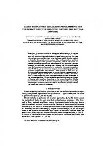
where Mi is the set indexes corresponding to the j-th eigenvalue of R (for example Mr+1 = {r + 1, · · · , m} for λr+1 ). Two representations of fˆm (x) for two different c and a sufficient large m are shown on Fig. 1 when the eigenvalues of R are 1, 2, 3, and 7 with the same multiplicity, where the eigenvalue 1 is the noise eigenvalue. One can observe that say (As6.S) is verified is equivalent to say that τn−1 > λ+ and τn+1 < λ− . In other words, all the sample eigenvalues corresponding to the non-unit eigenvalues of R, converge to a value τi which is outside the support of the Mar˘cenko-Pastur law (“asymptotic” PDF of the “unit” sample eigenvalues). As an illustration, one can notice that, in Fig. 1, for fˆm (x) plotted for c = 0.1, the separation condition √ is verified (ω1 = 6, ω2 = 2 and ω3 = 1 are greater that c = 0.316) and the three non-unit eigenvalues are represented on the PDF and outside the support of the Mar˘cenko-Pastur law by their respective limits τ1 = 7.116, τ2 = 3.15 and τ3 = 2.2. On the contrary, for fˆm (x) plotted for c = 1.5, only the two greatest eigenvalues are represented on the PDF by their respective limits τ1 = 8.75 and τ2 = 5.25 while the separation condition is not verified √ for the eigenvalue λ3 = 2 (ω3 = 1 < c = 1.223). In this case, the sample eigenvalues corresponding to the eigenvalue λ3 = 2 belongs to the Mar˘cenko-Pastur law.

5

one can deduce that with the spiked model and in the large dimensional regime: ˆ⊥ sH 1 Πc s2

a.s.

−→

m,K→∞

¯⊥ sH 1 Πc,S s2

(32)

m/K→c r ψi = 1 − χi , if i 6 r

(33)

ˆ −1 s2 is consistent in the two conConsequently, sH 1 R ˆ⊥ vergence regimes and, although sH 1 Πc s2 is consistent when K → ∞ with a fixed m, it is no more consistent under the regime of interest i.e. when both m, K → ∞ at the same rate. IV. N EW CONVERGENCE RESULTS A. Convergence of structured quadratic forms Fig. 1. PDF of the eigenvalues of the SCM with the spiked model when the eigenvalues of R are 1, 2, 3, and 7 with the same multiplicity, where 1 is the noise eigenvalue.

C. Convergence of simple quadratic forms

In this section, the convergence of the structured QF ˆ ⊥ is analyzed and results to Proposition 1. function of Π c Proposition 1: Let B be a m × m deterministic complex matrix with a uniformly bounded spectral norm for all m. Then, under (As1-As5, As6.S) and the spiked model, ˆ⊥ ˆ⊥ sH 1 Πc BΠc s2

Here, we compare the convergence of two QFs in two convergence regimes: when K → ∞ with a fixed m and when m, K → ∞ at the same rate. We first present the useful convergences of simple QFs ˆ It is well known that, due to the strong law function of R. ˆ → R of large numbers, when K → ∞ with a fixed m, R a.s. [38]. Thus, a.s.

−1 ˆ −1 s2 −→ sH sH s2 1 R 1 R

(27)

K→∞

a.s.

−→

m,K→∞

¯⊥ ¯⊥ sH 1 Πc,S BΠc,S s2

(34)

m/K→c